©2014 Science Publication
doi:10.3844/ajassp.2014.425.432 Published Online 11 (3) 2014 (http://www.thescipub.com/ajas.toc)
Corresponding Author: Ani Bin Shabril, Department of Mathematical Sciences, Universiti, Teknologi Malaysia, Skudai, Johor, 81310, Malaysia
DAILY CRUDE OIL PRICE FORECASTING MODEL USING
ARIMA, GENERALIZED AUTOREGRESSIVE CONDITIONAL
HETEROSCEDASTIC AND SUPPORT VECTOR MACHINES
1
Rana Abdullah Ahmed and
2Ani Bin Shabri
1,2
Department of Mathematical Sciences, Universiti Teknologi Malaysia, Skudai, Johor, 81310, Malaysia 1
Department of Mathematics, College of Basic Education, University of Mousl, Mousl, Iraq Received 2013-11-09; Revised 2013-11-19; Accepted 2014-01-11
ABSTRACT
Crude oil price forecasting is gaining increased interest globally. This interest is due mainly to the economic value attached to the product. For this reason, new forecasting methods are proposed in the literature. This paper proposes a novel technique for forecasting crude oil price based on Support Vector Machines (SVM). The study adopts the data on crude oil price of West Texas Intermediate (WTI) for its experimental purposes. This is because many studies have previously used this same data and it will afford a common basis for assessment. To evaluate the performance of the model, the study employs two measures, RMSE and MAE. These are used to compare the performance of the proposed technique and that of ARIMA and GARCH methods for the most efficient in crude oil price forecasting. The results reveal that the proposed method outperforms the other two in terms of forecast accuracy while it achieved a forecast error of 0.8684 that of ARIMA and GARCH were 0.9856 and 1.0134 respectively judging by their RMSE.
Keywords: Support Vector Machine, Forecasting, GARCH, Oil Price and ARIMA
1. INTRODUCTION
Forecasting crude oil prices is important as it affects other key sectors of the economy including the stock market. One of the important areas in economic research is forecasting the trend of price change of international crude oil. It is also a pointer in numerous industries for quick management intervention due to the recent extreme fluctuations in the price of international crude oil. This makes it crucial to develop reliable models that would assist adequately in forecasting the fluctuation of international crude oil price. This is aimed at facilitating the parties involved in taking appropriate action to avoid associated risk. The increase in price of international crude oil and its daily changes does not only affect the financial markets and economies, but it also affects individuals too. This is because of price increase of crude oil impacts greatly on the price of petrol which has its attendant effect on goods and services produced in the
country and by extension the gross domestic product (GDP). GDP has been defined by (Chrystal & Lipsey) as the total goods and services produced in a country within a given year. The aforementioned reasons makes the prediction of crude oil prices a very imperative task to decrease the impact of price fluctuations and assist policy makers and individuals to take informed decisions that would help in coping with price fluctuations arising from the energy markets. However, because of the mentioned reasons predicting crude oil is not a simple task. These have all made the prediction of the crude oil price a widely researched into area in the energy market. The models found in the literature on crude oil price forecasting include the popular Box-Jenkins method as in (Liu, 1991; Chinn et al., 2005; Agnolucci, 2009). Othermodels explored include GARCH-type models as in (Ahmed and Shabri, 2013; Hou and Saudy, 2012; Sadorsky, 2006). In this study, we attempt to extend the models used in the study of crude oil price to
the realm of the artificial intelligence particularly fitting a Support Vector Machine (SVM) to the forecast such data of high volatility.
Section 2 that follows this introduction discusses reviews of related works, Section 3 discusses the methodology in which we concentrate on the mathematical formulations of the three methods in this study and Section 4 discusses the results of the findings, while Section 5 gives the conclusion of the paper. Section 6 is devoted to acknowledgement in which we appreciated the assistance received from corporate bodies and individuals towards making this research come to light.
2. REVIEW OF RELATED LITERATURE
Liu (1991) employed Box-Jenkins technique to study the dynamic relationships between US crude oil prices, gasoline prices and the stock of gasoline with transferring function models US, while Kumar (1992) used time series models to investigate and compare the forecast accuracy of future prices of crude oil. The study fit an ARMA (1,2) model as the best fit model and compared with future crude oil prices with.The merits of ARIMA models are twofold (Wang et al., 2005). Initially, ARIMA models are a set of typical linear models which are proposed for the linear time series and captured linear characteristics in the time series. Subsequently, the theoretical base of ARIMA models is ideal.
Chinn et al. (2005) studied the predictive content of energy futures. They examined the relationship between spot and futures prices for energy commodities. An ARIMA (1,1,1) was used for crude oil prices forecast.
Sadorsky (2006) showed that the out-of-sample forecasts of a single equation GARCH model are best for those of Vector Auto-regression, state space and bivariate GARCH models, are more superior in forecasting the futures prices of petroleum. Agnolucci (2009) utilized diverse kinds of GARCH models and mentioned instability models to predict daily WTI future price instability, but the empirical results exposed that their performances were incompatible with regard to diverse measures and statistical tests.
Marzo and Zagaglia (2010) applied numerous GARCH models to predict the instability of daily futures prices of crude oil traded on NYMEX. The authors concluded they have not found a continuously greater model based on diverse statistical tests such as DM test, direction accuracy test and performance
measures as Success Ratio, Heteroscedasticity adjusted MSE, MAE and MSE.
Hou and Saudy (2012) an alternative approach involving nonparametric method to model and forecast oil price return volatility, the results demonstrate that the out-of-sample instability prediction of the nonparametric GARCH model defers greater performance qualified for a broad class of parametric GARCH models.
Ahmed and Shabri (2013) applied fitted GARCH model to crude oil spot prices. This was done in order to illustrate the advantages of nonlinear models. In the study the authors fit three GARCH models namely; GARCH-N, GARCH-t and GARCH–G to crude oil spot prices. The results revealed that GARCH-N model is the best model for forecasting for Brent while GARCH-G model is the best for forecasting of WTI crude oil spot prices.
Morana (2001) showed how the oil price allocation can be predicted by using the GARCH properties of oil price changes over short-term horizons. He used a semi-parametric approach to oil price forecasting and it was based on bootstrap approach. According to Marimoutou et al. (2009), the GARCH (1,1) -model may provide equally good results when compared to a combined GARCH and Extreme Value Theory (GARCH-EVT).
Sadorsky (1999) showed that oil price instability alarms have dissymmetrical effects on the financial system. The fluctuations in oil prices influence financial activity, but modification in financial activity has little impact on oil prices.
Most recently, Support Vector Machine (SVM) a novel neural network algorithm, was developed by Vapnik (1995) has gained significant inroad in the field of forecasting. Amongst the unique properties of SVM is that it is opposed to the over-fitting difficulty and can draw model nonlinear relations in a stable and efficient way. Additionally, SVM is instructed as a curved optimization problem resulting in the global explanation that in many cases defers exclusive explanations. Initially, SVMs have been expanded for categorization tasks (Burges, 1998). SVMs have been expanded to resolve time series prediction and nonlinear regression problems, with the introduction of Vapnik’s ε-insensitive loss function and they show excellent performance (Huang et al., 2005; Muller et al., 1997). Derived from this standard, SVMs will ultimately produce better simplification performance in comparison with other neural networks. Due to such
benefits, SVM method has been used in the area of economic time series forecasting (Tay and Cao, 2001; 2002; Kim, 2003; Huang et al., 2005). Whereas, in comparing with customary neural networks, the outstanding application of SVMs is derived from the state that the modeled data should have definite consistency. Accordingly, for the time series data with changing dynamics, a particular SVM model could not achieve well in capturing such dynamic and unstructured input-output relationship intrinsic in the economic data. Khashman and Nwulu (2011a) showed an intelligent system that forecasts the crude oil price. This intelligent system is derived from SVM, the outcomes gained were very hopeful as it established that SVM could be utilized with a high accuracy in forecasting the price of crude oil.
Xiao-Lin and Hai-Wei (2012) adopt three basic kernel functions of SVM to build the prediction model of the crude oil price, it used a particle swarm algorithm to optimize the parameters. The result show the prediction model whose parameters have been optimized by a genetic algorithm. Khashman and Nwulu (2011b) investigated and compared the applying of a back propagation neural network and an SVM to the task of forecasting oil prices and the outcomes propose the neural networks can be competently applied to forecast future oil prices with minimal computational expenditure.
3. THE METHODOLOGY
In this Section, the paper discusses the three techniques that feature prominently in this study. These are ARIMA, GARCH and SVM. Emphasis is laid on how the proposed SVM technique would be implemented in crude oil price forecasting.
3.1. ARIMA Modeling
Box and Jenkins (1976) introduced the ARIMA model and ever since then the method has turned out to be one of the most famous approaches to predicting. The future value of a variable in an ARIMA model is presumed to be a linear combination of past errors and past values, stated as follows:
t 0 1 t 1 2 t 2 p t p t 1 t 1 2 t 2 q t q y y y ... y ... − − − − − − = θ + φ + φ + + φ +ε − θ ε − θ ε − − θ ε (1)
where, yt is the actual value and φi and θj are the
coefficients, p and q are integers that are frequently submitted to as autoregressive, εt is the random error at time t and moving average polynomials, in that order. Fundamentally, this method has three stages: Model classification, parameter evaluation and diagnostic examination. For instance, the ARIMA (1,0,1) model can be characterized as follows Equation (2):
t 0 1 t 1 t 1 t 1
y = θ + φy− + ε − θ ε− (2)
Equation (1) demands some significant particular cases of the ARIMA family of models. If q = 0, then (1) becomes an AR model of order p. When p = 0, the model decreases to a MA model of order q. One essential task of the ARIMA model building is to conclude the suitable model order (p, q). According the previous work, Box and Jenkins (1976) developed a practical approach to building ARIMA models, which has the fundamental impact on the time series analysis and forecasting applications.
Box and Jenkins recommended to apply the Partial Autocorrelation Function (PACF) and the Autocorrelation Function (ACF) of the sample data as the fundamental tools to recognize the order of the ARIMA model. In the classification step, data transformation is frequently necessary to make the time series stationary. Stationarity is an essential stage in creating an ARMA model applied for predicting. A stationary time series is described by statistical characteristics for instance the mean and the autocorrelation structure being stable ultimately. While the experimental time series shows heteroscedasticity and trend, power transformation and differencing are used to the data to eliminate the trend and to become constant the variance before can be fitted an ARIMA model.
3.2. GARCH Modeling
The ARIMA (p, d, q) model cannot capture the heteroscedastic outcomes of a time series procedure, characteristically examined in the shape of high kurtosis, or gathering of volatilities and the influence effect. Engle (1982) initiated the Autoregressive Conditional Heteroscedastic (ARCH) model, afterward Bollerslev (1986) generalized it thus the name
Generalized Autoregressive Conditional Heteroscedastic model (GARCH). The term “conditional” implies the level of association on the past sequence of observations and the “autoregressive” describes the feedback mechanism that incorporates past observations into the present (Laux et al., 2011).
The variance equation of the GARCH (p, q) model can be expressed as Equation (3 and 4):
t Zt t Z ~ (0,1) ε = σ Ψ (3) p p 2 2 2 t t i t j i 1 j 1 2 2 t i t j i i (B) (B) − − = = − − σ = ω + α ε + β σ = ω + α ε + β σ
∑
∑
(4)where, Ψt (0, 1) is the likelihood density function of
the residuals or innovations with unit and zero mean variance. Intentionally, τ are extra distributional parameters to explain the shape and the skew of the distribution. The GARCH model can be reduced to the ARCH model if all the coefficientsβ are zero. Similar to ARMA models a GARCH requirement frequently guides to a more economical representation of the chronological dependencies and therefore presents a comparable additional flexibility over the linear ARCH model when parameterizing the conditional variance. Bollerslev (1986) has demonstrated that the GARCH (p, q) procedure is wide-sense stationary if the following conditions hold:
• E(εt) = 0 • var( )t (1 (1) (1)) ω ε = − α − β
• cov( ,ε εt s), t≠s if and onlyif (1)+(1)<1
The simple GARCH (1, 1) model has been established to offer a good demonstration of an extensive diversity of volatility procedures in most applications, (Bollerslev et al., 1992).
3.3. Support Vector Machines
Vapnik (1995) proposed the Support Vector Machines (SVMs). According to the Structured Risk Minimization (SRM) principle, SVMs look for reducing an upper bound of the generalization error rather than the empirical error as in other neural
networks. Furthermore, the SVMs models create the revert function by concerning a set of high dimensional linear functions. The SVM regression function is formulated as follows Equation (5):
y(x)= φw (x)+b (5)
where, Φ(x) is named the feature, which is nonlinear planed from the input space x. The coefficients w and b are evaluated by minimizing Equation (6 and 7):
N 2 i i i 1 1 1 R(C) C L (d , y ) w N = 2 =
∑
ε + (6) i i d y d y L (d , y ) 0 others ε − − ε − ≥ ε = (7)where, both C and ε are prescribed parameters. The first term Ls(di, yi) is named the ε-intensive loss
function. The di is the actual stock price during the ith
period. This function shows that errors below are not penalized. Also the term (
N z i i i 1 C(1 N) L (d , y ) =
∑
measuresthe empirical error. The next term, 1 w2
2 is the flatness of the function. C assesses the trade-off between the flatness of the model and the empirical risk. ξ and ξ* were introduced as the positive slack variables, which signify the distance from the actual values to the corresponding boundary values of ε-tube. Equation (4) is converted to the following constrained formation:
Minimize:
(
N)
T * i i i 1 1 R(w, , *) ww C * ( ) 2 = ξ ξ = +∑
ξ + ξ (8) Subjected to Equation (9 to 11): * i i i i w (x )φ +b −d ≤ ε + ξ (9) i i i i d − φw (x )−b ≤ ε + ξ (10) * i i whereξ ξ ≥0,i=1, 2,..., N (11)Finally, introducing Lagrange multipliers and maximizing the dual function of Equation (8) we have:
N N * * * i i i i i i i i 1 i 1 N N * * i j j j i j i 1 j 1 R( ) d ( ) ( ) 1 ( ) ( )K(x , x ) 2 = = = = α − α = α − α − ε α − α − α − α × α − α
∑
∑
∑∑
(12)With the constraints Equation (13 to 15):
N * i i i 1 ( ) 0 = α − α =
∑
(13) i 0≤ α ≤C (14) * i 0 C i 1, 2,..., N ≤ α ≤ = (15)In Equation (12), αi and αi* are called Lagrangian
multipliers. They satisfy the equalities Equation (16):
* * i i l * i i i i 1 * 0 f (x,a,a*) ( )K(x, x ) b = α α = α − α +
∑
(16)Here, K(x, xi) is named the kernel function. The
amount of the kernel is equivalent to the inner product of two vectors xi and xj in the feature space φ(xi)
and φ(xj), such that K(x, xi) = φ(xi)*φ(xj). Any
function that fulfilling Mercer’s condition Vapnik (1995) can be applied as the kernel function. The Gaussian kernel function:
(
2 2)
i j i j
K(x , x )=exp − x −x / 2σ
Is specific in this study. The SVMs were used to evaluate the nonlinear behavior of the predicting data set because Gaussian kernels aim to present good performance under common efficiency assumptions.
3.4. Proposed SVM Implementation
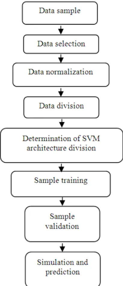
The flowchart of the proposed SVM technique is shown in Fig. 1. This gives a vivid illustration of the procedure for expanding an SVM for time series predicting. The flowchart in Fig. 1 can be split into four phases. The first phase is data sampling. To expand an SVM model for a predicting training,
scenario, testing and validating data require data collection. Although, the data collected from a variety of sources must be chosen along with the equivalent norms. Sample preprocessing is the second phase that comprises of two steps: First step involves data normalization and second step is data division. In the process of developing any model, familiarity with the accessible data is one of the greatest significance. SVM is no exception to this rule, as well; data normalization n can influence model performance significantly. Subsequently, data collection should be divided into two sub-sets: First in-sample data and second out-of-sample data which are applied for model development and model evaluation in that order. SVM training and learning is the third phase. This phrase comprises three major tasks: Determination of SVM architecture, sample training and sample validation, which is the center procedure of the SVM model.
SVM-based crude oil price forecasting involves four steps:
• Data sampling. For this research various data can be collected, for example NYMEX, WTI. Data collected can be classified into diverse time scales: Daily, weekly and monthly. For daily data, there are a variety of missing points and inconsistencies for the marketplace has been blocked or stopped because of unexpected events or weekends. Consequently, weekly data and monthly data should be approved as alternatives
• Data preprocessing. It may require to be transformed the collected oil price data into a definite suitable range for network learning via logarithm transformation, variation or other methods. After that the data should be split into out-of-sample data and in-sample data
• Training and learning. In this step the training results determine the SVM architecture and parameters. There are no norms in choosing the parameters other than a trial-and-error basis. In this study, the RBF kernel is applied because the RBF kernel tends to provide good performance under common softness assumptions
• As a result, it is particularly constructive if no extra information of the data is accessible. In conclusion, an acceptable SVM-based model for oil price predicting is attained.
• Future price forecasting
Selecting corresponding SVM parameters is the modeling: Kernel function and penalty factor c, which influence significantly on the predicting outcomes. Statistical software was used to create evaluation among sigmoid kernel function, radial basis function, kernel function and polynomial kernel function. In conclusion, the radial basis function was selected for the high prediction accurateness and concurrently through many trials of the parameter computation.
3.5. Data
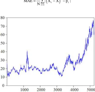
For this study, the West Texas Intermediate (WTI) crude oil spot price was adopted for experimental purposes. The reason of choosing the oil price signs is that, the crude oil prices are the most well-known standard prices, which are extensively applied at the
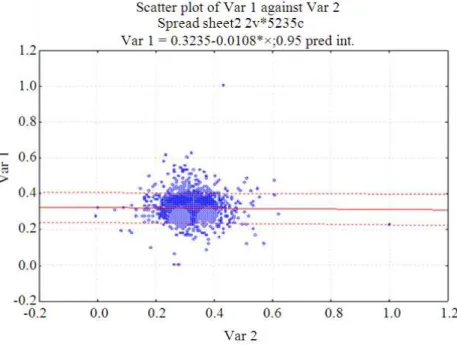
foundation of many crude oil price codes. The crude oil price data utilized in this study are daily data and are generously available from the energy information administration (EIA).The data covers the period January 1, 1986 to September 30, 2006, thereby giving a total of 5237 observations. The data is presented in Fig. 2. A difference in unit can result in a difference in data magnitude, which tends to affect prediction accuracy in the long run. The normalization processing can resolve this issue. In this study, the data was normalized to a scalable range of [0,1] in the training set and prediction set, using the normalization equation:
(
) (
)
n i min max min
X = X −X / X −X
The normalized data is shown in Fig. 3.
3.6. Evaluation of Volatility Forecasts
This study adopted two very popular measures for evaluating the forecast accuracy of the series and these are: Mean Absolute Error (MAE) and Root Mean Square Error (RMSE). These measures are evaluated by assessing their returns. The one with the lowest error measure is judged the best. These measures are defined as follows.
Mean Absolute Error (MAE) is given by:
(
)
N 2 t t t 1 1 ˆ MAE | X X p | N = =∑
− −Fig. 3. The normalized data for WTI Table 1. The evaluation of forecasting results for WTI crude
oil price
Methodology RMSE MAE
ARIMA 0.9856 0.7204
GARCH 1.0134 0.7392
SVM 0.8684 0.6304
and Root Mean Squared Error (RMSE) is given by:
(
)
(
)
1/ 2 2 t t k t 1 1 ˆ RMSA x x p N = =∑
− − Where:Xt : The return of the horizon before the current time t
X : The average return t
ˆp : Is the forecast value of the conditional variance over n steps ahead horizon of the current time t
3.7. Results and Analysis
The results are shown in Table 1.
From Table 1 it can be seen that the proposed method SVM outperforms GARCH and ARIMA techniques. From the point of view of the RMSE it returned a forecast error of 0.8684 followed by ARIMA with a forecast error of 0.9856 and then GARCH with 1.0134. For the MAE SVM still post the best result with forecast accuracy of 0.6304; ARIMA 0.7204 and GARCH 0.7392.
4. CONCLUSION
In this study a novel approach based on artificial intelligence for crude oil price modeling is proposed. The proposed technique forecast accuracy performance was evaluated using two measures of error RMSE and MAE and compare with some other well-known techniques in crude oil spot price forecasting like ARIMA and GARCH. The results reviewed that the proposed SVM method outperforms the others. The study therefore recommends that the proposed SVM method be employed in future for crude oil price forecasting.
5. REFERENCES
Agnolucci, P., 2009. Volatility in crude oil futures: A comparison of the predictive ability of GARCH and implied volatility models. Energy Econ., 31: 316-321. DOI: 10.1016/j.eneco.2008.11.001
Ahmed, R.A. and A.B. Shabri, 2013. Fitting GARCH models to crude oil spot price data. Life Sci. J., 10: 654-661.
Bollerslev, T., 1986. Generalized autoregressive conditional heteroskedasticity. J. Econometr., 31: 307-321. DOI: 10.1016/0304-4076(86)90063-1 Bollerslev, T., R.Y. Chou and K.F. Kroner, 1992. ARCH
modeling in finance ☆: A review of the theory and empirical evidence. J. Econ., 52: 5-59. DOI: 10.1016/0304-4076(92)90064-X
Box, G.E.P. and G. Jenkins, 1976. Time Series Analysis: Forecasting and Control. 1st Edn., Holden-Day, San Francisco, ISBN-10: 0816211043, pp: 575.
Burges, C.J.C., 1998. A tutorial on support vector machines for pattern recognition. Data Mining Knowl. Discovery, 2: 121-167. DOI: 10.1023/A:1009715923555
Chinn, M.D., M.R. LeBlanc and O. Coibion, 2005. The Predictive Content of Energy Futures: An Update on Petroleum, Natural Gas, Heating Oil and Gasoline. 1st Edn., National Bureau of Economic Research, pp: 17.
Engle, R.F., 1982. Autoregressive conditional heteroscedasticity with estimates of the variance of united kingdom inflation. Econometrica, 50: 987-1007.
Hou, A. and S. Suardi, 2012. A nonparametric GARCH model of crude oil price return volatility. Energy
Econ., 34: 618-626. DOI:
10.1016/j.eneco.2011.08.004
Huang, W., Y. Nakamoria and S. Wang, 2005. Forecasting stock market movement direction with support vector machine. Comput. Operat. Res., 32: 2513-2522. DOI: 10.1016/j.cor.2004.03.016
Khashman, A. and N.I. Nwulu, 2011a. Intelligent prediction of crude oil price using support vector machines. Proceedings of the IEEE 9th International Symposium on Applied Machine Intelligence and Informatics, Jan. 27-29, IEEE Xplore Press,
Smolenice, pp: 165-169. DOI:
10.1109/SAMI.2011.5738868
Khashman, A. and N.I. Nwulu, 2011b. Support vector machines versus back propagation algorithm for oil price prediction. Proceedings of the 8th International Conference on Advances in Neural Networks, May 29-Jun. 01, Springer Verlag Berlin, Guilin, China, pp: 530-558. DOI: 10.1007/978-3-642-21111-9_60 Kim, K.J., 2003. Financial time series forecasting using
support vector machines. Neurocomputing, 55: 307-319. DOI: 10.1016/S0925-2312(03)00372-2
Kumar, M.S., 1992. The forecasting accuracy of crude oil futures prices. Int. Monetary Fund, 39: 432-461. DOI: 10.2307/3867065
Laux, P., S. Vogl, W. Qiu, H.R. Knoche and H. Kunstmann, 2011. Copula-based statistical refinement of precipitation in RCM simulations over complex terrain. Hydrol. Earth Syst. Sci., 15: 2401-2419. DOI: 10.5194/hess-15-2401-2011
Liu, L.M., 1991. Dynamic relationship analysis of us gasoline and crude oil prices. J. Forecast., 10: 521-547. DOI: 10.1002/for.3980100506
Marimoutou, V., B. Raggad and A. Trabelsi, 2009. Extreme value theory and value at risk: Application to oil market. Energy Econ., 31: 519-530. DOI: 10.1016/j.eneco.2009.02.005
Marzo, M. and P. Zagaglia, 2010. Volatility forecasting for crude oil futures. Applied Econ. Lett., 17: 1587-1599. DOI: 10.1080/13504850903084996
Morana, C., 2001. A semiparametric approach to short-term oil price forecasting. Energy Econ., 23: 325-338. DOI: 10.1016/S0140-9883(00)00075-X Muller, K.R., J.A. Smola and B. Scholkopf, 1997.
Predicting time series with support vector machines. Proceedings of the International Conference on Artificial Neural Networks, Oct. 8-10, Switzerland, pp: 999-1004. DOI: 10.1007/BFb0020283
Sadorsky, P., 1999. Oil price shocks and stock market activity. Energy Econ., 21: 449-469. DOI: 10.1016/S0140-9883(99)00020-1
Sadorsky, P., 2006. Modeling and forecasting petroleum futures volatility. Energy Econ., 28: 467-488. DOI: 10.1016/j.eneco.2006.04.005
Tay, E.H. and L.J. Cao, 2001. Application of support vector machines in financial time series forecasting. Omega, 29: 309-317. DOI: 10.1016/S0305-0483(01)00026-3
Tay, F.E. and L.J. Cao, 2002. Modified support vector machines in financial time series forecasting. Neurocomputing, 48: 847-861. DOI: 10.1016/S0925-2312(01)00676-2
Vapnik, V.N., 1995. The Nature of Statistical Learning Theory. 1st Edn., Springer, New York, ISBN-10: 0387987800, pp: 314.
Wang, S.Y., L.A. Yu and K.K. Lai, 2005. Crude oil price forecasting with TEI@I methodology. J. Syst. Sci. Complexity 18: 145-166.
Xiao-Lin, Z. and W. Hai-wei, 2012. Crude oil prices predictive model based on support vector machine and particle swarm optimization. Proceedings of the International Conference on Software Engineering, Knowledge Engineering and Information Engineering, (SEKEIE ‘12), pp: 645-650. DOI: 10.1007/978-3-642-29455-6_89