Direction and Intensity of Technical Change: a Micro Model

in Economia

No. 4 (February 20, 2009)

Direction and Intensity of Technical

Change: a Micro Model

The Doctoral School of Economics

The Doctoral School of Economics is an academic structure that organizes and coordinates the activities of five doctoral programs in economics and related fields in "La Sapienza".

The School's main goals

 the creation of an integrated system of postgraduate teaching;

 the formation of highly skilled researchers in a multidisciplinary perspective;

 to provide a better visibility to postgraduate teaching;

 to facilitate the students' mobility overseas;

 to establish forms of collaboration with national and international institutions. The five PhD programs of the School

 International Monetary and Financial Markets (Economia dei Mercati Monetari e Finanziari internazionali)

 Economics (Economia Politica)

 Mathematics for Economic-Financial Applications (Matematica per le applicazioni economico-finanziarie)

 Economic Sciences (Scienze Economiche)

 Economic Statistics (Statistica Economica) Editorial board of the Working Papers

Maria Chiarolla; Rita D’Ecclesia; Maurizio Franzini; Giorgio Rodano; Claudio Sardoni; Luigi Ventura; Roberto Zelli.

Direction and Intensity of Technical

Change: a Micro Model

Luca Zamparelli



Abstract

This paper develops a growth model combining elements of endogenous growth and induced innovation literatures. In a standard induced innovation model firms select at no cost innovations from an innovation possibilities frontier describing the trade-off between increasing capital or labor productivity. The model proposed allows firms to choose not only the direction but also the size of innovation by representing the innovation possibilities through a cost function of capital and labor augmenting innovations. By so doing, it provides a micro-foundation both of the intensity and of the direction of technical change. The policy analysis implies that an increase in subsidies to R&D as opposed to capital accumulation raises per capita steady state growth, employment rate and wage share.



Keywords Induced innovation, endogenous growth, direction of technical change JEL Classification: O31, O33, O40.

Direction and Intensity of Technical Change: a Micro Model

1

Introduction

More than forty years ago, Kaldor (1961) singled out the constancy of the output-capital ratio and the steady increase of the labor productivity as two of the main stylized facts characterizing western industrialized economies. With medium run fluctuations, these facts have been confirmed till the current years (see for example Romer 1989 and Evans 2000). Two questions arise: first, why technical change is biased towards labor augmentation; second, what accounts for the extent of labor productivity increases. The standard neoclassical growth model, though compatible with these facts, provides no answer to each of the questions. Harrod neutrality is assumed as the only kind of technical change compatible with the existence of steady states, and the magnitude of the growth rate of technology is also a given.

Determining endogenously the rate of technical change in a model based on the neoclassical theory of distribution was indeed problematic. Under perfectly competitive conditions, factors of productions are paid according to their marginal productivities. This implies that under constant returns to scale in labor and capital the whole product is just sufficient to pay their remuneration, and nothing is left to reward the cost of introducing an innovation.

The endogenous growth literature has overcome this impasse. Leaving aside the human capital and AK models and focusing on R&D driven technical change, two alternatives have been explored. In the early 90s the abandonment of perfect competition and the introduction of a degree of monopoly into growth models provided the rents necessary to justify a costly research activity; models of horizontal (Romer 1987, 1990) and vertical (Grossman and Helpmann 1991, Aghion and Howitt 1992) innovation have been developed by adopting this framework. Abandoning the assumption of constant returns to scale in production while retaining perfect competition provided a second option. Under decreasing returns to scale competitive firms earn positive profits in equilibrium; such profits may be used to pay for the cost of innovation. Recent contributions have developed this possibility (Hellwig and Irmen 2001, Irmen 2005). However, the endogenous growth literature in its various forms simply assumed that innovations would improve labor productivity thus neglecting (with the notable exception of Acemoglu 2002, 2003, 2007) the issue of the direction of technical change.

2

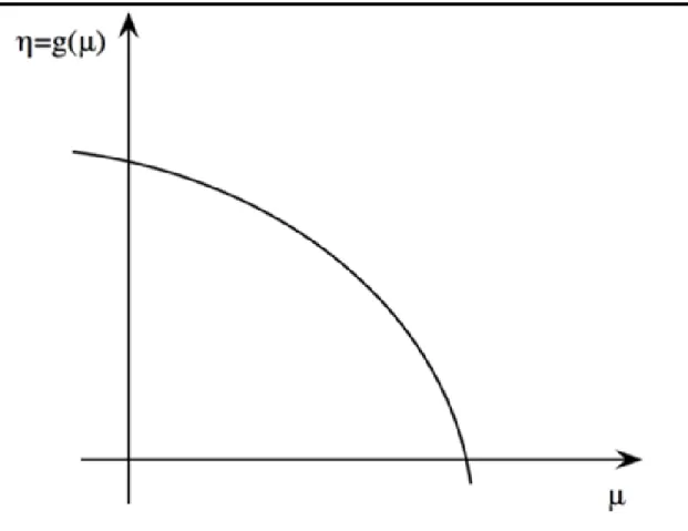
The idea that market mechanisms may influence the direction of change in technology traces back at least to Hick’s (1932, pp. 124-5) suggestion that technical change would tend to economize the factors becoming relatively expensive. Theorists of the 60s (von Weizsacker (1962), Kennedy (1964), Samuelson (1965) and Drandakis and Phelps (1966)) formally developed this intuition. In particular, this literature known as ‘induced innovation’ introduced an innovation frontier to describe the trade-off between growth rates of labor and capital productivity available to the firm. Figure 1 represents the original formulation of the innovation possibility frontier put forward by Kennedy as the function  g( ) , where  is the rate of growth of capital productivity and  is the rate of growth of labor productivity; all the points below the curve represent couples of rates of growth of labor and capital productivity freely available to the firm. Firms are assumed to choose a combination of factors productivity augmentation in order to maximize the current rate of unit cost reduction given factors employment and prices. The maximization problem solution implies that the direction of technical change depends on factors shares: the market economy has an endogenous tendency to save the factor of production whose share is increasing. Provided that the elasticity of substitution between labor and capital is smaller than one, the economy converges to a steady state equilibrium with constant factors shares and pure labor-augmenting technical progress. In turn, Harrod neutral technical change finds an explanation rooted in the economic behavior of firms. From an empirical point of view, the induced innovation hypothesis seems to be confirmed by, or at least is consistent with, the positive reaction of labor productivity growth to an increase in the labor share that seems to characterize most industrialized countries (see Gordon 1987, Barbosa-Filho and Taylor 2006).

Direction and Intensity of Technical Change: a Micro Model

Figure 1 Innovation possibility frontier

In these models however, the position of the innovation possibility frontier was assumed to be given so that the steady state growth rate of labor productivity was necessarily exogenous.

Working within R&D models based on imperfect competition Acemoglu (2002, 2003, 2007) has been able to endogenize at the same time the direction and the intensity of technical change. I attempt a similar procedure in a model that combines neoclassical elements, such as perfect competition and convexity of individual costs structure, with classical ones such as the division in classes (workers, capitalists and entrepreneurs) and a non-clearing labor market. While the interest rate brings about the equality between demand and supply in the loanable funds market, the employment rate depends only on technology and on the level of productive capacity. In the spirit of the induced innovation literature the existence of a possibility frontier is assumed; however, it is not given exogenously. Its position depends on firms’ investment, and innovating is therefore costly: the model provides a microfoundation of both the direction and the size of innovation.

4

A steady state solution with constant output-capital ratio, labor productivity growth, factors shares and employment ratio is derived. The main finding is that, contrary to Acemoglu’s results, fiscal policy is effective: an increase in subsidies to R&D increases steady state per capita growth, wage share and employment ratio.

2

The Model

2.1 Individual firm

We start by considering the static problem of the firm at time t. Firms produce a homogeneous output and are price takers; at time t each firm faces the problem of choosing the level of capacity x_{i t} , and the one period growth rates of augmentation of capital and labor efficiency

( _{i t} _{i t}) which will determine the firm’s technology at time t 1 At t 1, given capacity and the state of technology the firm will hire the profit maximizing mass of labor n_{i t 1} Output at

1

t  is given by the Leontief production function Y_{i t 1} min[x b_{i t t} (1_{i t}) (1a_t _{i t} )n_{i t 1}] where b_t and a_t are respectively the level of efficiency reached by capital and labor in the economy at time t. Notice thatb_t and a_t are not indexed by i since innovations are assumed to be freely available after one period of monopoly.

Direction and Intensity of Technical Change: a Micro Model

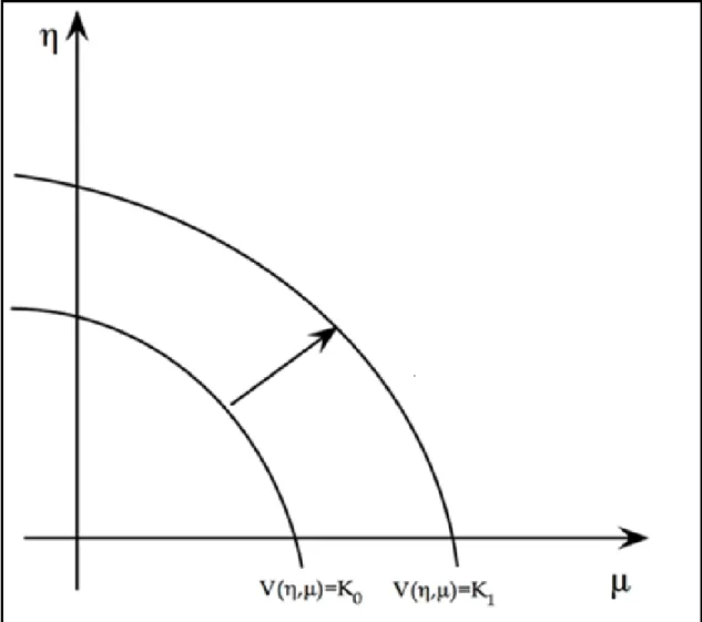
Technology characterization requires the specification of the cost function of productive capacity and innovation. In order to increase capacity from x_t1 to x_t (I assume no depreciation) the firm has to invest the amount K x x( _t _t1) of output. The innovation technology is such that by investing V(  Y_i) units of output each firm can improve the technology from (b a_t _t) to

( (1b_t  ) (1a_t )). The functionV is intended to allow the technological frontier to become endogenous. The technological frontier represents the tradeoff between the possibility of augmenting capital or labor efficiency; it is usually assumed to be exogenous and given at a certain level. With the aid of the cost function introduced we can represent a whole family of technological frontiers as the level curves associated to different levels of R&D spending. Figure

6

2 shows the level curves of the cost function of innovation associated to the level of investment 0

K , K₁.

In order to work out the solution to our problem we make the following assumptions:

1 1 1

( _{t t} ) _t ( _{t t} )

K x x _ x _ x x_

(.)

 is twice continuously differentiable with:



 







 

21 2 1 (1) (1) 0, / , / 0 , , _{i i} , t t t t x x x x V  Y YC    _                 (.)

C is twice continuously differentiable with:

(0 0) 0, ( ) 0 C   C    otherwise (0 0) 0 ( ) 0 C C         otherwise 2 _{( )} D C   is positive definite.

Notice that the cost function for innovation is not defined in the negative quadrant as past technologies are freely available to the firm. Moreover, both for capacity and innovation, we have assumed zero marginal cost at the origin to assure positive investment. As usual in the literature of investment cost, the assumption of convexity can be justified through the idea of adjustment costs, and it is necessary in order for the static optimization problem to be well-defined. Moreover, the cost functions of innovation and capacity are scaled respectively to initial output and to initial capacity to avoid that the unit cost of increasing productivity or capacity would asymptotically tend to zero.

Since production emerges only at period t1, firms have to borrow at time t to pay for the cost of investment in capacity and innovation; they will pay the interest rate i_t upon the amount of output borrowed.

Profit maximization requires n_{i t 1} x b_{i t t 1}a_t1 so that the profit maximization problem at t is

Direction and Intensity of Technical Change: a Micro Model 1 1 1 , , 1 1 1 1 [ (1 ) (1 ) (1 ) ( ) (1 ) ( )] (1 ) [1 (1 ) ] (1 ) ( ) ( ) it it it e t i t t it t it it t t it it i t i t i t x e it t it t it t t t i t it it i t i t i t Max Y w b x a i V Y i K x x b x w a i b x C x x x                                            _      _     _

with   (0 1] being the discount factor. Notice that today’s profit maximizing plan depends on the expected level of the wage rate as today’s choice of capacity in fact fixes the amount of labor the firm will decide to hire in the next period.

Given the assumptions onV and K the maximand function is strictly concave and the first order conditions are sufficient and necessary for a maximum:

1 1 (1 ) [1 e (1 ) ] (1 ) ( ) 0 it t t it t t i t i t it b w a i x x x          _{          }      (1) 1 1 [1 e (1 ) ] (1 ) _t( ) 0 t it t it t t t i t it it it b x w a i b x C_          _{        }      (2) 2 1 1 (1 ) e (1 ) (1 ) _t( ) 0 t it it t it t t t i t it it it b x w a i b x C_           _{        }      (3)

Let us define the labor share as  Then _t w a_{t t} and w a_te_{1 t} _te_1 is the expected labor share. Notice that the labor productivity level considered to calculate the expectation on tomorrow’s labor share is today’s productivity a_t. It is so as firm i will have a one period monopoly over the technology it develops and, at the same time, firms do not take into account the possibility that their own behavior might be adopted by the rest of firms population. e_t1 becomes the key variable in choosing innovation direction. Using (2) and (3) we get:

1 2 1 [1 (1 ) ] 1 (1 ) (1 ) 1 1 (1 ) ( ) ( ) (1 ) e t it t e it t it t e w a it t it it it e w a it it it t C C                 _    _  _                  or in a simpler fashion 1 1 ( ) 1 1 1 ( ) e it it it t it e it it it t C C_         _      _   (4)

The observation of (4) confirms the result of the directed technical change literature. An increase in the wage share has to be accommodated by increasing labor productivity more than

8

capital productivity. There is a tendency in the market system to introduce a bias in the technical change towards the factor whose share is increasing. A sufficient condition for this result is

( _{it it}) ( _{it it}) ( _{it it}) ( _{it it})

C_   C_   C_   C_   . The condition requires that the level curves of the cost function representing the trade-off between capital and labor augmentation corresponding to different levels of R&D spending be concave: i.e. it is analogous to the assumption of concavity of the innovation possibility frontier1.

2.2 Closure of the model

In order to move to the macroeconomic equilibrium we assume a representative firm. Along classical lines it is also assumed that workers consume all their wages and capitalists save their whole income and offer it on the financial market to earn the interest rate i.

For a given expectation on the wage share e_t1 and interest rate i_t the firm’s maximization problem determines the equilibrium values:

1 1 1 1 1

{ ( e ) ( e ) ( e ) ( e )}

t t t t t t t t t t t t

x  i   i   i n  i

       

Solving for the equilibrium of the economic system at a certain point in time requires that we specify the equilibrium conditions for the interest rate and the wage rate, together with the way expectations on the wage rate are determined.

The role of the interest rate is to clear the output market. It will assume the value at which the excess of output over workers’ consumption (the economy’s saving) is fully invested in either innovation or capacity:

1 1 t t ( ( e 1 ) ( e 1 ) ) ( ( e 1 ) 1) t t t t t t t t t t t t t t t t b x Y b x w V i i Y K x i x a                         (5) 1

Consider the level k of expenditure in innovation. Then we have C(   ) k By totally differentiating

2 2 2 2 2 2 0 so that 0 In turn, and C d C d C d C k d C d C k C C C C d C C C C C d C k d C                                             

Direction and Intensity of Technical Change: a Micro Model

Current production is consumed either as workers’ consumption or as investment in innovation and capacity.

Since labor demand at a certain point in time is determined by the previous period profit maximizing investment in capacity and technical change there is no guarantee that the labor market will clear. In turn: Lb x_{t t t1} a_t, where L_t is the (inelastic) labor supply at time t. Let us assume that labor market tightness influences the expectation on next period wage rate, and let such tightness be measured by the employment rate v_t   n L_{t t} b x_{t t1} (a L_{t t}). Then, expectations on the wage rate can be modeled according to

1 ( )

e

t t t

w_  f w v (6)

with f fwt  vt 0

Finally, we impose that in equilibrium expectations are correct

1 1

e

t t

w w

   (7)

For any initial condition_a b x_{0 0 1}_

 

   

2

we have six conditions (1), (2), (3), (5), (6), (7) to determine a sequence of temporary equilibrium values for six endogenous variables

1 1

( e )

t t t t t t

x     w w i_ _  Notice the different nature of the prices of labor and capital. The interest rate adjusts instantaneously to clear the market of loanable funds while the wage rate is determined by its past history and the disequilibrium on the labor market in the previous period.

2.3 Dynamical System

The evolution of the equilibrium can be represented as a system of difference equations in the three state variables (b v_t  _t _t) If we define the function h v( )_t w_t1w_t  f w v( _t _t) w_t, the expected wage share can be expressed as e_t1 h v( )_t _t. From equation (2 bis), the interest rate can be obtained as a function of the three state variables: i_t i b v(_t _t _t). In turn we have the following system:

2_{To keep notation consistent I have denoted}

1

x_ the initial capacity the representative firm is endowed with at the beginning of timet .

10 1 1 1 1 (1 ( ( ) ) (1 ( ( ) ))( ( ( ) ))(1 ( ( ) ))(1 ) ( )1 ( ( ) ) t t t t t t t t t t t t t t t t t t t t t L t t t t t t t b b h v i v v h v i x x h v i h v i g h v h v i                                        (8)

where g_L is the exogenous rate of population growth. The system determines the evolution of the capital productivity, employment ratio and labor share. In the process, the remaining endogenous variables (_{t t}   i _t x_t) are determined as functions of the state variables and the parameters describing technology and the labor market.

2.3.1 Steady state

Stationary equilibrium requiresb_t b_t1 b_ss; v_t v_t1 v_ss; _t _t1 _ss. The system becomes:





( ) ₀ ( ) ( ) ( ) 1 1 1 ( ) ( ( ) ( ) 1 ( ) ss ss ss ss ss ss ss ss ss ss x ss L ss ss ss ss ss ss ss ss ss ss ss ss ss h v i b v h v h v g g i b v i b v h v h v i b v     _                _{ }    _   _     (9)

where g_x is the steady state growth rate of capacity. Using (9) and dividing (5) by Y_t the equilibrium conditions can be rewritten as:

[1 ] (1 ) ((1 ) ( )) ss ss ss L ss b _ _{  }i  _g h v _{(1 bis)} (1g h v_L) ( )[1_ss _ss] (1 i C_ss) (0 ( ) 1)_ h v_ss  (2 bis) (1g_L)_ss  (1 i C_ss) (0 ( ) 1)_ h v_ss  (3 bis) ((1 ) ( )) 1 (0 ( ) 1) L ss ss ss ss g h v C h v b         (5 bis)

Solving for (1i_ss) in (3 bis) and for b_ss dividing (1 bis) by (2 bis) and by plugging

Direction and Intensity of Technical Change: a Micro Model (0 ( ) 1) ( ) (0 ( ) 1) ss (0 ( ) 1) ( )ss ss ss ss ss C h v h v C_ h v  C_ h v h v         

The steady state value for the labor share is always economically meaningful being positive and smaller than one. Using _ss in (3 bis) and 1 (bis) we obtain:

(1 ) ( ) (0 ( ) 1) (0 ( ) 1) ( ) (1 ) L ss ss ss ss g h v ss C h v C h v h v i _  _        and (1 ) ( ) ((1 ) ( )) (0 ( ) 1) L ss L ss ss g h v g h v ss C h v b  _     

Finally, substituting for b_ss and _ss into (5 bis) determines implicitly h v( )_ss .

(0 ( ) 1) ( ) 1 (0 ( ) 1) (0 ( ) 1) ( ) (0 ) (1 ) ( ) (0 ( ) 1) (1 ) ( ) (1 ) ( ) ss ss ss ss ss ss L ss ss L ss L ss C h v h v C h v C h v h v C g h v C h v g h v g h v                          (10)

After b_ss _ss v_ss and i_ss have been determined, (9) solves for _ss h v( ) 1_ss  and

(1 ) ( )

x L ss

g  g h v . Notice also that since Y_t1 x b_{t t}(1_t) the steady state growth rate of output is

L

y x ss

g g g   , i.e. the equality between the warranted and natural growth rates. Notice however that the growth rate of labor productivity is endogenous both as it is determined as the profit maximizing decision of the firm, and, as we will see in Section 4, as it can be affected by the action of the policy maker.

Using the definition of profits we can calculate the steady state level of the profit rate as: 1

( ) [(1 )(1 ) (1 )( )]

ss t t ss ss x ss ss ss

r   x_ b g   i C   b , which, given (5 bis), implies

(1 )( )

ss ss ss x ss

r b  g i . The gross profit rate of the economy, b_ss(1_ss)g_x, is divided between the remuneration of the interest on saving and the residual compensation of the entrepreneurs. Entrepreneurs profits are positive if and only if the rate of growth of the economy exceeds the interest rate. This possibility arises from the restriction to entry in production. In

12

fact, as it is customary in general equilibrium analysis (see MacKenzie, 1959), equilibrium extra-profits can be conceived of as a rent rewarding the fixed factor entrepreneurship.

3

Discussion of the Model

Several papers in recent years have provided microfoundations of growth models under perfectly competitive conditions. I have adopted a framework similar to the one developed by Bester and Petrakis (2003), Hellwig and Irmen (2001), and Irmen (2005) which assumes perfect competition and strictly convex investment cost in capacity and innovation. In these models the assumption of convexity is fundamental as increasing marginal costs provide the equilibrium inframarginal rents necessary to pay for the cost of innovation. At the same time, even when the innovation possibility frontier is exogenous and only the direction of technical change is chosen by the firm (see Funk, 2002), convexity is necessary to assure that the individual firm’s production plan be bounded. In my model, since no free entry is assumed, there exist positive profits part of which can be used to finance the cost of innovation. Therefore convexity simply guarantees that the investment plan is finite.

Also like in Hellwig and Irmen (2001) and Bester and Petrakis (2003) I assume Leontief production function. However, contrary to those models, even though at a given point in time there is zero substitutability between factors, by directing innovation towards either factors of production firms can use technical change to substitute one factor to the other. Much in the spirit of Kaldor’s (1957) suggestion to abolish the neoclassical distinction between movements along the production function due to capital deepening, and shifts of the production function due to technical change, technical progress is required to change factors proportion. A similar idea has been developed by Foley and Michl (1999) and Michl (1999) through the concept of fossil

production function. They show that a pattern resembling a smooth neoclassical production

function with capital deepening can be obtained as the trace of successive adoptions of labor saving and capital using technical change. My model differ from their approach as firms do not face an exogenous labor-saving capital-using evolution of technology but choose both the size and the direction of innovation.

The dynamical system of employment rate, wage share and capital productivity described in (8) can be seen as a Goodwin (1967) growth model generalized to encompass the possibility of

Direction and Intensity of Technical Change: a Micro Model

endogenous direction of technical change. It has been first studied by Shah and Desai (1981) and later analyzed by van der Ploeg (1987), Thompson (1995), Foley (2003) and Julius (2005) among the others. They have shown that, once coupled with the innovation possibility frontier, the cyclical behavior of the Goodwin model collapses to a stable steady state with constant factor shares, capital productivity and growth rate of labor productivity. Under one respect my system is fundamentally different. Since the innovation possibility frontier is endogenous the steady state productivity growth and income distribution are not uniquely pinned down by the innovation technology but they depend on the incentive to accumulate. As we see in the next Section 4 this opens up the possibility for policy action.

4

Policy Analysis

The per-capita growth rate of the economy in the standard neoclassical model is exogenous. This exogeneity is to be understood in a twofold way. On the one hand, the growth rate is exogenous as technical change is not the outcome of profit-maximizing agents’ decision. On the other hand, it is independent of the propensity to save and, in turn, it cannot be affected by the action of the policy maker.

Section 2 developed the ‘descriptive’ model where growth is endogenous as it is the result of firms’ investment in innovation. This section shows that, in our model, growth is endogenous as the policy maker can affect the steady state per capita growth by means of tax/subsidy to investment in innovation and capital accumulation.

Let  be the tax/subsidy rate on investment in R&D, and let  be the tax/subsidy rate on capacity investment. (  ) will represent a tax if   0, and a subsidy in case    0 Subsidies on investment are financed through lump sum taxes on capitalists’ saving; analogously, in case of a positive tax rate, taxes on investment are transferred to capitalists. The fiscal budget remains unaffected. Let A 1  and B  1 , the model (1 bis - 5 bis) becomes

[1 ] (1 ) ((1 )(1 ))

ss ss ss L ss

b _ _{ }i B_ _g _ _{(1 tris)}

14 (1g_L)_ss  (1 i AC_ss) _(0 )_ss (3 tris) ((1 )(1 )) 1 (0 ) L ss ss ss ss g C b           (5 tris)

where we used h v( ) 1_ss   _ss Notice that equation (5 tris) is not affected by the policy action: a change in the cost of investment at the right hand side

( (0 )C _ss    ((1 g_L)(1_ss))b_ss) cancels out at the left hand side with an equivalent

change in the economy’s saving.

Proceeding analogously to what we did to find (10) we obtain:

(0 ( ) 1) ( ) 1 (0 ( ) 1) (0 ( ) 1) ( ) (0 ) (1 ) ( ) (0 ( ) 1) (1 ) ( ) (1 ) ( ) ss ss ss ss ss ss L ss ss L ss L ss C h v h v C h v C h v h v C g h v C h v g h v g h v                          (11)

In the attempt to prove our result let us start by considering the case where only innovation is targeted by the policy maker. We set in turn B 1 in (9). By totally differentiating and rearranging we find 2 (1 _L)(1 _ss) ( (1 _ss) )(1 _L)(1 _ss) C_ g  dA C _ A C_  C_ g         _      _   _ 2 2 2 ( )(1 _ss) (1 _ss) (1 _ss) AC_      C C_{  } C C_{  }  C C C_{ } _ C_   d         _  _ _   _{ }   where we used the fact that in steady state d 0

In turn, since the concavity of the isocosts of the innovation production implies C C_{  } C C_{  } , a sufficient condition for d 0

dA  is given by C(1ss)C and

2 



   . Under such conditions a reduction in the cost of innovation fosters steady state per capita growth

The subsidy to innovation also affects income distribution and employment. In steady state, we have

Direction and Intensity of Technical Change: a Micro Model ( ) 1_{ss ss} h v   and (0 )(1 ) (0 _ss) ss(0 _ss)(1ss _ss) C ss C_  C_        _{ } _ _ ; since h  () 0 and (1 ) ₂ 0 1

(

)

ss ss ss ss C C C C C C d d C C                    _{ }         



_











, by increasing the

steady state rate of growth of labor productivity, a subsidy to innovation raises the labor share and the employment ratio.

Analogously, we can study the effect of a change in the subsidy to capital accumulation on the steady state per capita growth rate. Since B enters equation (11) in exactly the same way as

1

A, it follows necessarily that signdBd  signdAd  In turn, the sufficient conditions derived

before guarantee d 0

dB  : reducing the cost of capital accumulation reduces steady state per

capita growth.3

Our policy analysis has shown that, under plausible conditions, steady state per-capita growth can be fostered both by subsidizing innovation and by taxing capital accumulation.

5

Conclusions

The paper provides a proposal to unify endogenous growth and induced innovation literature. With firms allowed to choose both the direction and the size of innovation, the productivity

3

To appreciate the non-restrictiveness of this condition consider as an example

1 t t x x      _ _   , with 0, 1

  to assure strict convexity; and C

 

 , a



2 2



c, with ,a c0, a symmetric positive definite quadratic form. Under this assumption the sufficient conditions for a positive impact of an increase in subsidy to

R&D is always satisfied as

 

2 2 2 2 2 2 2 2 2 2 2 1 1 1 1 0 t t t t t t x x x x x x                       _ _   _ _  _ __        , and



1



0 C  C  c (where we used  0.

16

growth rate is not uniquely pinned down by technology. The policy maker is capable of affecting the economy’s performance in terms of steady state growth and income distribution and employment by subsidizing either innovation or capital accumulation.

Direction and Intensity of Technical Change: a Micro Model

References

Acemoglu, D. (2002), ‘Directed Technical Change’,Review of Economic Studies, 69, 781-810. Acemoglu, D. (2003), ‘Labor- and Capital-Augmenting Technical Change’,Journal of European

Economic Association, 75 (4), 1371-1409.

Acemoglu, D. (2007), ‘Equilibrium Bias of Technical Change’,Econometrica, 1, 1-37

Aghion, P. and P. Howitt (1992), ‘A Model of Growth through Creative Destruction’,

Econometrica, 60(2), 323-51.

Barbosa-Filho, N. and L. Taylor (2006), ‘Distributive and Demand Cycles in the US Economy- a Structuralist Goodwin Model’,Metroeconomica, 57 (3), 389–411.

Bester, H. and E. Petrakis (2003), ‘Wages and Productivity Growth in a Competitive Industry’,

Journal of Economic Theory, 109 (1), 52-69.

Drandrakis, E. and E. Phelps (1966), ‘A Model of Induced Invention, Growth, and Distribution’,

Economic Journal, 76, 823– 40.

Evans, P. (2000), ‘US Stylized Facts and Their Implications for Growth Theory’, WP.

Foley, D. (2003), ‘Endogenous Technical Change with Externalities in a Classical Growth Model’,Journal of Economic Behavior and Organization, 52, 201-233.

Foley, D. and T. Michl (1999), Growth and Distribution, Cambridge, MA, Harvard University press.

Funk, P. (2002), ‘Induced Innovation Revisited’,Economica, 69, 155-171.

Gordon, R. J. (1987), ‘Productivity, wages, and prices inside and outside of manufacturing in the US, Japan, and Europe’,European Economic Review, 31, 685-733.

Gordon, R. J. (2000), ‘Interpreting the ‘One Big Wave’ in US long-term Productivity Growth’,

CEPR No. 2608.

Goodwin, R. (1967), ‘A Growth Cycle’, in Socialism, Capitalism and Economic Growth, C. Feinstein ed., Cambridge, MA, Cambridge University Press.

Grossman, G.M. and E. Helpman (1991), ‘Quality Ladders in the Theory of Growth’, Review of

Economic Studies58, 43-61.

Hellwig, M. and A. Irmen (2001), ‘Endogenous Technical Change in a Competitive Economy’,

Journal of Economic Theory, 101 (1), 1-39.

Hicks, J.R. (1932),The Theory of Wages,London: Macmillan, 1960.

Irmen, A. (2005), ‘Extensive and Intensive Growth in a Neoclassical Framework’, Journal of

18

Julius, A.J. (2005), ‘Steady-State Growth and Distribution with an Endogenous Direction of Technical Change’,Metroeconomica, 56(1), 101-125.

Kaldor, N. (1961), ‘Capital Accumulation and Economic Growth’, in Lutz, F. A. and Hague, D.

C.The Theory of Capital, New York, St. Martin’s press.

Kennedy, C. (1964): ‘Induced Bias in Innovation and the Theory of Distribution’, Economic

Journal, 74, 541–47.

McKenzie, L. (1959) ‘On the existence of a general equilibrium for a competitive market’,

Econometrica, 27: 54-71.

Michl, T.M. (1999), ‘Biased Technical Change and the Aggregate Production Function’,

International Review of Applied Economics, 13.

Romer, P. (1987), ‘Growth Based on Increasing Returns Due to Specialization’, The American

Economic Review Papers and Proc.77.

Romer, P.M. (1989), ‘Capital Accumulation in the Theory of Long-Run Growth’, in Barro, R. J.

Modern Business Cycle Theory, Cambridge, MA, Harvard University Press.

Romer, P.M. (1990), ‘Endogeneous Technological Change’, Journal of Political Economy 98, S71-S102.

Samuelson, P. (1965), ‘A Theory of Induced Innovation along Kennedy–Weizsäcker Lines’,

Review of Economics and Statistics, 47, 343–56.

Shah A. and Desai (1981), ‘Growth Cycles with Induced Technical Change’,Economic Journal, 91, 977-987.

Thompson, F. (1995), ‘Technical Change, Accumulation, and the Rate of Profit’, Review of

Radical Political Economy, 27, 97-126.

van der Ploeg, F. (1987), ‘Growth Cycles, Induced Techincal Change, ad Perpetual Conflict over the Distribution of Income’,Journal of Macroeconomics, 9 (1), 1-12.

von Weizsäcker C. C. (1966), ‘Tentative Notes on a Two-Sector Model with Induced Technical Progress’,Review of Economic Studies, 95, 245–52.

5.1 Heading 2