ISPRS Int. J. Geo-Inf. 2019, 8, 367; doi:10.3390/ijgi8090367 www.mdpi.com/journal/ijgi Article
Application of Remote Sensing Data for Evaluation
of Rockfall Potential within a Quarry Slope
Carlo Robiati 1,*, Matt Eyre 1, Claudio Vanneschi 2, Mirko Francioni 3, Adam Venn 4
and John Coggan 1
1 Camborne School of Mines, University of Exeter, Penryn TR10 9FE, Cornwall, UK 2 CGT Spinoff Srl, Via Vetri Vecchi 34, 52027 S. Giovanni Valdarno, AR, Italy
3 Department of Engineering and Geology, University of Chieti-Pescara, Chieti 66100, Italy 4 Imerys Minerals Ltd., St Georges Rd in Nanpean PL26 7XR, Cornwall, UK
* Correspondence: [email protected]
Received: 12 July 2019; Accepted: 19 August 2019; Published: 22 August 2019
Abstract: In recent years data acquisition from remote sensing has become readily available to the quarry sector. This study demonstrates how such data may be used to evaluate and back analyse rockfall potential of a legacy slope in a blocky rock mass. Use of data obtained from several aerial LiDAR (Light Detection and Ranging) and photogrammetric campaigns taken over a number of years (2011 to date) provides evidence for potential rockfall evolution from a slope within an active quarry operation in Cornwall, UK. Further investigation, through analysis of point cloud data obtained from terrestrial laser scanning, was undertaken to characterise the orientation of discontinuities present within the rock slope. Aerial and terrestrial LiDAR data were subsequently used for kinematic analysis, production of surface topography models and rockfall trajectory analyses using both 2D and 3D numerical simulations. The results of an Unmanned Aerial Vehicle (UAV)-based 3D photogrammetric analysis enabled the reconstruction of high resolution topography, allowing one to not only determine geometrical properties of the slope surface and geo-mechanical characterisation but provide data for validation of numerical simulations. The analysis undertaken shows the effectiveness of the existing rockfall barrier, while demonstrating how photogrammetric data can be used to inform back analyses of the underlying failure mechanism and investigate potential runout.
Keywords: rockfall hazard; slope stability; remote sensing; LiDAR; SfM-MVS; photogrammetry
1. Introduction
Rock fall during quarrying activities are among the most critical risks associated with slope instability, especially for high cuts in weathered rock [1]. Legacy slopes, such as the one studied in this investigation, may be particularly prone to rockfall, since they were created prior to the UK Quarry Regulations (1999) [2] and regular maintenance may be difficult to undertake. Rockfall is a slope process involving the detachment of rock fragments and their fall and subsequent bouncing, rolling, sliding, and deposition, where the main responsible factor for the rockfall behaviour is the slope inclination and its irregularities [3,4,5]. Cruden and Varnes [6] define rockfall as a failure where “little or no shear displacement takes place and the material descends mainly through air in free-fall, leaping, bouncing or rolling. Movements are very rapid and may or may not be preceded by minor movements leading to progressive separation of the rock mass from its source.” According to McCauley [7], the main cause for the initiation of rockfalls can be directly related to water, namely rain, snow-melt, springs and seeps, and the associated increased pressure due to water infiltration in pores and discontinuities. The triggers and conditions that instigate rockfall that are not directly
related to water are root wedging, excavation activities and earthquakes, and these can account for a significant portion of the observed rockfall failures [8]. Rockfall instability phenomena, in natural and engineered slopes, have been under investigation since 1960s, and the results have been published by a large number of researchers; dealing with the physical basis of the process [9,10,11,12], and the hazard and risk associated with it [13,14,15,16].
In the last two decades, developments in the area of geo-information, in particular in the production of three-dimensional models, has enhanced the ability to carry out rockfall risk assessments in previously inaccessible locations. In addition, workflows have been defined based on the acquisition of 3D point clouds and the extraction of the information that they contain [17,18,19,20,21,22]. Depending upon the frequency of data acquisition and the rate of change of the slope prior to its failure it is possible to hypothesise the slope failure mode, the potential volume of the eventual failure and, in some cases, provide an accurate estimate of the time of failure [23]. In back analysis, it is possible to determine the position of the source areas, to assess the path of movement or trajectory, to calculate the volume of accumulated debris, and the velocity and energy associated with its descent [24]. Point clouds produced directly with laser scanning (LiDAR), terrestrial (TLS) or aerial (ALS) [25,4,26,27] or produced by means of applying Structure from Motion Multi-View Stereo (SfM-MVS) algorithms, using platforms as Unmanned Aerial Vehicle (UAV) [28,29,30,31] can play a fundamental role in the characterisation of rockmass quality and its features. Indeed, both TLS and UAV are easy and fast to operate, allowing one to acquire data with high geometric and temporal resolutions. The identification and localisation of discontinuities enable detailed spatial modelling of these structures that can be used as input parameters for numerical simulations of rock slope stability.
This study provides a rockfall evaluation for a legacy slope in an active open pit operation through back-analysis of the rockfall using remotely captured data. Legacy slopes often do not comply with the most recent regulations, in terms of acceptable geometry (height and profile) and maintenance (not being subject to regular scaling), so the uncertainty of parameters associated with triggering and predisposing factors, as well as purely geometric characteristics (frequency and distribution of discontinuities) render such analyses challenging. However, the availability of high resolution remotely captured datasets (ALS, TLS and SfM-MVS derived point clouds), obtained from surveying campaigns routinely carried out in active mining operations can be of key importance for defining the geological conditions and structures that promote rockfall events. Through definition of the slope’s geo-mechanical characteristics and incorporation of this information in a GIS environment, using 2D and 3D numerical simulations, a rockfall reach probability map showing the location and distribution of modelled rockfall has been produced. The influence of the spatial resolution of the surface topography on the modelled behaviour is also investigated. The simulations were run using an array of topographic models at different resolutions to investigate the effect of grid size on the run-out of rock blocks. A specific test was designed to study the effect of rock blocks’ shape in the 3D simulations. Part of this investigation is also to ascertain if the protection measures are adequately designed to mitigate the risk resulting from further potential detachments from the rock face. The study demonstrates the benefits of using probabilistic numerical models, both in two and three dimensions, in order to reduce the uncertainty arising from the difficulties of validating results in inaccessible areas. As far as the Authors are aware, there are no studies showing a direct comparison of rockfall trajectory analysis models in 2D and 3D, and how this comparison can lead to a more reliable assessment of rockfall hazard.
Case Study: The Treviscoe Rockfall
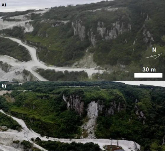
The case study is based on back analysis of a rockfall event that initially occurred in 2011, developed into a full slope scale activity in 2013, including a major event in early 2016 with further ongoing activity. The rockfall is located in a section of a quarry bench in Treviscoe Pit, St.Austell, UK (Figure 1a–c). The site location requires a detailed analysis, given that the internal geotechnical assessment suggests that it poses a significant hazard, as per the UK Quarry Regulations (1999) [2]. Treviscoe Pit is located within the St. Austell granite cupola, in SW England. The pit, from which both
kaolinite (china clay) and aggregates are extracted, is one of the oldest in the region, resulting in an excavation 600 by 300 m and approximatively 80 m in depth. The rockfall has undergone several different phases of activity, as reported by mine personnel. In order to reduce the risks associated with rockfall, a rock trap was created at the base of the slope to prevent blocks from reaching the haul road.
As can be observed in Figure 2a, b, which illustrates the conditions at the slope prior (2013) and after (2018), the major collapse event occurred in early 2016, and the outcrop presents itself as a fairly irregular sub-vertical rock face. The material outcropping is a weathered topaz-bearing granite [32,33], which has undergone partial to complete kaolinisation. The rockmass appears to contain near vertical columnar joints, spaced 1 m, resting on basal planes gently dipping towards the free face. The sub-vertical wall is approximately 21 m in height. At the base of the sub-vertical section is a slope with a bench angle of approximately 50° that consists of vegetation and scree. The scree is the result of several rockfall events depositing material towards the bottom of the slope. To protect and mitigate against rock fall a sand bund was erected at the base of the slope, approximately 3 m in height, along the whole section of the haul road.
Figure 1. Location of the rockfall slope (a) aerial location of the case study position in the overall pit; (b) localised aerial view; (c) view from the base of the slope. The photographs were acquired in August 2018. Scale bar in (c) is indicative.
Figure 2. Photographic comparison of the rockfall (a) October 2013 and (b) August 2018. The photos were taken from the opposite side of the pit, circa 300 m away from the target and they show the change in geometry due to the major collapse occurred in early 2016. Scale bar is indicative.
2. Materials and Methods
In order to investigate and evaluate the rockfall events several data collection surveys were undertaken and are summarised below. The obtained datasets were utilised to inform different types of analyses, extracting key geo-mechanical parameters and to constrain numerical modelling simulations, i.e., 2D and 3D rockfall trajectory analysis.
2.1. Close-Range Remote Sensing Survey
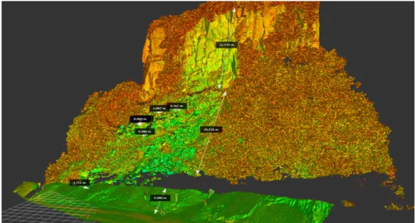
To generate a DEM (Digital Elevation Model) and to extract geo-mechanical information for the rockfall numerical simulations, two remote sensing techniques were selected to capture the scene at close-ranges: TLS and drone-borne SfM-MVS. Given the restrictions posed by the hazardous conditions on the rock wall, the position on the ground from where the LiDAR unit could be operated were limited. The most reasonable choice to overcome this condition after the initial scans was to opt for a drone-based survey, with the capacity of getting closer observations, hence improving the GSD (Ground Sampling Distance), and eventually allowing to capture some previously shadowed zone of the slope, as the top of the cliff and the inner side of the rock-trap. The TLS survey was carried out with a Leica ScanStation C10™, a time-of-flight laser scanner with a nominal scan resolution, at ranges from 0 to 50 m, of 4.5 mm, with an accuracy on a single measurement position and distance of 6 and 4 mm, respectively. The rock face was scanned in May 2017 with a Leica ScanStation C10™, from four individual scan positions, approximatively 35 m away from the target, to obtain a high
resolution point cloud of 27 × 106 points, with an average spacing of 0.025 m (shown in Figure 3). The
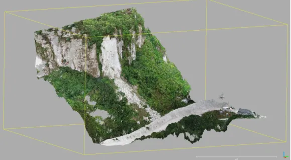
same manufacturer as the aforementioned LiDAR unit. The TLS point cloud was oriented to magnetic North with the help of a compass bearing. The root-mean-square error (RMSE) on the z coordinate for the point cloud registration is 0.017 m. A second survey was performed in August 2018, as soon as a UAV was available to the mine operation survey team, and a second high resolution point cloud reconstructed by means of SfM-MVS workflow, using optical images taken from a drone. The dataset for the SfM-MVS scene reconstruction was obtained with a DJI Phantom 4 Pro™, using the built-in 20 MP camera with mechanical shutter, controlled remotely by the drone operator. The drone was flown manually, at an average distance of ~20 m from the rock face, acquiring 303 images and using four fixed GCP (Ground Control Point) present in the observed scene. GCP network was established by the mine survey department, having their coordinates measured using D-GNSS (Differential-Global Navigation Satellite System). The point cloud was processed in Agisoft Photoscan™, resulting
in a point cloud of 19 × 106 points, with an average point spacing of 0.029 m (shown in Figure 4).
Other than a DEM, as an output from the SfM-MVS workflow, a high resolution RGB orthophoto was generated, having a GSD of 0.0073 m. The orthophoto was generated at the highest possible resolution to enable a detailed mapping of the rockfall debris.
Figure 3. Registered TLS (terrestrial laser scanning) point cloud image, with illustrative sample dimensions highlighting the sub-vertical rock wall and the scree slope. Given the inaccessibility of the inner side of the rockfall trap, the TLS was unable to capture its complete geometry. Some sample measurements were taken and highlighted as to show the indicative vertical drop from the source area to the base of the slope, and the length of the scree slope/transition zone. The same measurements were used to obtain a representative block size on the rock wall.
Figure 4. Coloured Structure from Motion Multi-View Stereo (SfM-MVS) point cloud image, acquired using a Phantom 4 DJI platform equipped with a 20 MP RGB camera and processed in Agisoft Photoscan™. The Unmanned Aerial Vehicle (UAV)-hosted sensor enabled the complete reconstruction of shadowed regions in the scene in the TLS survey.
2.2. Long-Range Remote Sensing Survey
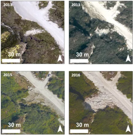
The mining operation, through a contractor, had previously undertaken a series of aerial laser scanning (ALS) derived point cloud, capturing the geometry of the entire pit at 1 m ground sample distance (GSD). The error associated with the z coordinate for the surveys did not exceed 0.070 m for all the campaigns (2011, 2013, 2015, 2016) with a RMSE of 0.060 m that resulted from averaging the RMSE in z of the four campaigns, computed over 52 GCP scattered across the mining operation, i.e., the local reference grid used by the surveying personnel. The multi-temporal, yearly, LiDAR coverage (2011 to 2016) provided the basis to reconstruct the variation in geometry of the pit walls over time. The ALS surveys were performed in the same flights designed to acquire aerial photographs. In this study, aerial photographs served the purpose of changing detection analysis, and to constrain, both temporally and geometrically, the evolution of the rockfall. The orthorectified aerial images (shown in Figure 5) were generated with a GSD of 30 cm and the surveyor’s ground truth report indicates a RMSE on the xy plane of 0.15 m. In Figure 5, a series of orthorectified images (from 2011 to 2016), it can be observed how the rockfall, after the initial activity in 2011, occurred through further release events.
The ALS, TLS and SfM-MVS point clouds were rasterised in CloudCompare™, using the rasterize tool, to generate DEM with different grid sizes; using ALS data for GSD above 1 m, TLS data for GSD of 1 m, finally SfM-MVS derived data for topographical models below 1 m GSD. In this way there several DEM, having 5, 2, 1, 0.5 and 0.3 m grid sizes were produced.
Figure 5. Orthorectified aerial imagery of the rockfall area. The sequence shows the activity of the rockfall, from its initial condition (top left), to the development of the rockfall at the whole slope scale in 2013 (top right), and the subsequent maintenance operations, the emplacement of the rock trap and the removal of rock fragments from the ditch. The last picture shows the aftermath of the major collapse that led to the actual slope geometry.
2.3. Geo-Mechanical Analysis
In potentially hazardous environments, such as a legacy slope, it is not possible to carry out traditional geo-mechanical surveys due to the unacceptable level of risk the surveyors would be exposed to. Technological advancements in remote mapping platforms have helped to overcome this issue, as reviewed in Tannant [34] and Giordan [30], resulting in a rapidly growing market of reliable, low cost UAV. It has been previously shown that surface topography reconstructed with TLS and SfM-MVS methods can be successfully used to determine the orientation and spacing of rock discontinuities [35]. In order to obtain a statistically robust representation of the discontinuities in the outcropping rockmass, the TLS point cloud was processed and analysed in SplitFX™. This software is designed to extract geo-mechanical information from point clouds by mapping either planar facets or trace planes and subsequently plotting them on a stereoplot. The TLS point cloud data was imported into SplitFX and the discontinuities mapped by manually assigning best fit polygons onto the point cloud surface. The point normal of the polygon can then be represented on an equal area hemispherical stereonet to identify discontinuity sets and perform kinematic analysis for potential failure mechanisms.
The orientation of the rock discontinuities captured within SplitFX was then imported in DIPS™, and a kinematic analysis was performed [36,8]. The analysis of source areas for rockfall includes identification of kinematically admissible unstable blocks and an investigation of the factors influencing the stability of such blocks [37]. The Markland test [36] considers the possible slope failure mechanisms, without considering forces, and has been used to establish some possible rockfall scenarios for further numerical simulation.
2.4. GIS Geospatial Analysis
The geospatial datasets (aerial ortho-photographs, ALS, TLS and SfM-MVS derived DEM) were incorporated in the ESRI ArcGIS™ environment for the purpose of establishing a database of the information related to the rockfall event. The aerial photography coverage from 2011 to 2016 (Figure 5) and the digital photogrammetric survey (both the high resolution orthorectified image and the SfM-MVS derived DEM), enabled the mapping of the activity of the main rockfall scarp, other than the end locations of rock blocks. The aerial imagery time series also served the purpose of recording the effects of maintenance operations, i.e., the creation of the sand embankment protecting the haul road and the removal of rock fragments trapped in the rockfall ditch. The GIS environment provided the platform to analyse and map, in high-resolution, homogeneous areas, namely the (a) source area, the (b) scree slope, the (c) vegetated slope and the (d) rock-trap, shown in Figure 6. GIS evaluation also provided the chance to record the position of end point locations for validation of subsequent rockfall simulations. The spatial analysis toolbox provided means for managing DEM, from which a representative vertical cross section (profile) was taken (shown in Figure 6) for subsequent numerical modelling.
The GIS also formed the basis for pre-processing the rasters used as topography for the 2D (by extracting a vertical profile) and 3D (as an ASCII DEM) numerical simulations through assigning input parameters to the different homogeneous areas mapped, as described in the Section 3.3.
Figure 6. Geo-mechanical zonation used to assign input parameters for the 3D numerical modelling. In red is shown the trace of the representative vertical profile extracted from the Digital Elevation Model (DEM) to obtain the slope geometry for 2D numerical modelling.
2.5. Numerical Modelling
An established method to assess the hazard posed by rockfalls is the use of probabilistic rockfall trajectory analysis [38,39]. A probabilistic approach is adopted to consider both ontic and epistemic
uncertainty in rockfall trajectory modelling, i.e., the variability of the information gathered during the surveying phase of the study and the preparation of GIS data layers [39,37]. To produce a realistic simulation of the rockfall behaviour, the models must incorporate a digital representation of the topography, either in the form of a DEM raster or a vertical profile, both of which can be retrieved from remotely sensed data. The topography gradient will govern the general direction that a block will take through its descent. Predefined physical-mechanical characteristics of the digital surface are used to compute the loss of energy for the inelastic rebounds with the ground at each pixel of the DEM. These parameters are called Coefficients of Restitutions (COR), defined as an energy transfer function, which is generally expressed in the form of a ratio between the velocity before and after an impact [40,41]. COR are defined in the normal direction (CORN) and tangential (CORT) to the slope. They are used to account for energy lost due to the inelastic deformation during the collision of a rock with the slope or bench [42]. COR are key parameters for rockfall modelling, and it is necessary to use engineering judgement when selecting appropriate values from literature, especially given the inherent difficulties of defining them empirically through field testing [43,9,41].
A common distinction in how rockfall modelling software treats impact theory is the lumped mass (LM) approach versus the rigid body (RB) approach. The lumped mass approach considers the mass being concentrated in a single point, while the rigid body approach uses a defined geometry to model the rock block. Due to ongoing activities in the pit it was not possible to undertake in-situ field calibration tests for assessing directly the reliability of the models and the effectiveness of the rockfall protection [44,45]. However, validation was obtained from comparison of modelling results with aerial images of the rockfall body and known end locations for rockfall fragments. COR values for the two-dimensional lumped-mass impact model (2DLM) were obtained from literature and compared with a soil cover map of the site.
In this study two software were selected to perform the trajectory analyses: Rocfall™, developed by Rocscience, and Rockyfor3D™, developed by ecorisQ Association. They were selected as they are reliable tools, largely used both in academia and in the industry. In addition, they offer different solutions in terms of statistical assumptions and results typology.
Rocfall™ is a 2D-LM (Lumped Mass) probabilistic, processed-based software for rockfall simulation [46] reproducing the trajectory of rock blocks falling along a 2D slope. The input parameters (i.e., CORN, CORT, static friction, rolling dynamic friction and slope roughness) can be obtained from literature and previous calibrated simulations or example data from the help documentation in the software itself. The software then allows definition of the statistical variability of these input parameters [39]. The point cloud geometries were used as the basis to provide a representative sectional line for simulation. A representative vertical section (shown as a red trace in Figure 6) was generated from both the ALS, TLS and SfM-MVS point clouds and exported into AutoCAD™ to provide the geometry for subsequent 2D rockfall simulations. The vertical section was extracted at different geometrical resolution using the 3D Analyst toolbox in ArcGIS™.
The vertical sections were then traced to form a polyline in AutoCAD™, which was then exported into Rocscience Rocfall™ for analysis. A sensitivity analysis on the slope geometry resolution was undertaken, extracting the topography from ALS, TLS and SfM-MVS derived DEM, at 5, 2, 1, 0.5 and 0.3 m.
Rockyfor3D™ is a three-dimensional rigid-body impact model (3D-RB) (Rigid Body) that calculates trajectories of single, individually falling rocks with discrete geometry (RB), in three dimensions (3D). The model combines physically-based, deterministic algorithms with stochastic approaches, which makes Rockyfor3D a so-called ‘probabilistic process-based rockfall trajectory model’. Rockyfor3D can be used for regional, local and slope-scale rockfall simulations [47]. In this software the input parameters are assigned to the digital surface through pre-processing of ASCII GIS data layers (i.e., release cells location, density, shape and dimensions of rock blocks and their statistical variation range and initial vertical velocity). The local slope surface roughness is represented by a parameter defined as maximum obstacle height (MOH), expressed in metres. Typical MOH values, as suggested by Dorren [47], which are encountered by a falling rock are represented by statistical classes, namely rg70%, rg20%, and rg10%. During each rebound calculation,
the MOH value in a cell is randomly chosen from the three representative values according to their probabilities of occurrence [47]. A sensitivity analysis on the influence of the DEM resolution was performed for the case study, comparing the results of the rockfall (blocks) end point(s) when using a DEM having a 5, 2, 1, 0.5 and 0.3 m GSD and for different rockfall size scenarios, for 2D-LM and 5, 2 and 1 m for 3D-RB simulations.
3. Results
Following the remote sensing data collection campaigns, the collected data were processed in several software applications to generate the products which were used to classify the slope and evaluate the potential of a rockfall at the site.
3.1. Geo-Mechanical Analysis
Figure 7 illustrates an example of a discontinuity mapping carried out on the point cloud in SplitFX. The mapping identified 348 different entries that were then exported into Rocscience DIPS™ to identify the major discontinuity set orientations characterising the rock mass and to perform kinematic analysis. Figure 8 illustrates the kinematic analysis undertaken in DIPS, where the principal discontinuity sets were identified. Table 1 summarises the major sets orientations represented using Dip and Dip Direction format. The stereographic analysis confirmed the presence of near vertical columnar joints represented by Sets 1 and 2 and basal planes (Sets 3 and 4) dipping out of the face.
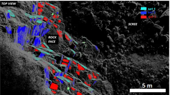
Figure 7. Top view of the rock wall. The coloured facets highlight the discontinuity network identified in Figure 8. The blue and teal patches identify joint Sets 1 and 2, responsible for isolating columnar-like prisms and acting as release planes. The red patches identify the joint Set 3, acting as a basal plane. Set 4, in green, is rarely mapped because of its geometrical orientation (near horizontal). Scale bar is indicative.
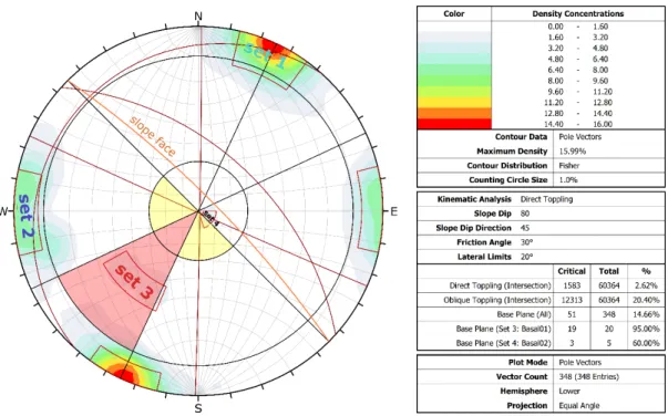
Figure 8. DIPS Stereoplot representation of the discontinuities extracted with SplitFX. The area shaded in red and yellow represents the area of instability highlighted by the kinematic analysis for direct and oblique toppling. The colour code associated with joint sets reflects the mapping performed on SplitFX in Figure 7.
Table 1. Summary of the geometrical orientation of the main joint sets identified in SplitFX. Joint Set Mean Dip (°) Stdv (°) Mean Dip Direction (°) Stdv (°)
1 86.3 3.1 205.7 5.1
2 85.5 2.7 89.7 9.7
3 53.6 2.6 41.0 12.8
4 9.3 1.9 313.5 19.1
It can be seen from the kinematic analysis that the discontinuity mapping has highlighted the potential for both direct and oblique toppling from the slope, assuming a friction angle of 30°. In addition, the point cloud was used to establish typical block dimensions that could be formed by the respective discontinuity sets and be released in the event of rockfall. This was achieved by using the TLS point cloud and taking measurements perpendicular to the set orientation to obtain a true spacing and an estimate of the persistence [35]. The typical block size distribution comprises blocks
ranging from 10 cm to 2 m in width. The rockfall deposit is scattered across an area of circa 430 m2,
and a visual comparison, aided by the measurement of blocks within the point cloud data, gives an
estimated value for the total mobilised rock mass to be approximately 250 m3.
In Figure 8 the result of the kinematic analysis for direct and oblique toppling are provided. The analysis is computed on 348 digitally mapped planar rock facets, assuming a general slope dip of 80°, the slope dip direction of N 45°, a standard friction angle of 30°, and lateral limits of 20°. The DIPS analysis shows how 20.24% of the discontinuities intersections potentially leading to oblique toppling fall into the instable area of the plot (shaded in red), justifying the assumed style of deformation for the case study.
3.2. 2D Rockfall Trajectory Analysis (Rocfall 2D-LM)
In this section the outcome of the 2D Lumped Mass rockfall trajectory analysis is presented. The input COR parameters used in the simulation are shown in Table 2. The COR were selected based on
the literature available and the database values suggested by the software developer (literature value ± 3 stdv). Release points (or linear seeders) for the rockfall events were positioned at various locations at the top of the slope and along the sub-vertical rock wall. These source locations were validated through direct observation of relative fresh rockfall scars in the field and with the aid of high-resolution optical images (single close range frames from the drone survey). The overall number of rocks released from the seeders for each simulation run (5, 2, 1, 0.5 and 0.3 m resolution) was 10,000. Using the spacing and rock size distribution analysis performed previously, three rock classes, summarised below in Table 3, were selected for simulating different scenarios. The initial conditions of the blocks, in terms of initial horizontal and vertical velocity, were kept as default, i.e., zero angular and linear initial velocity.
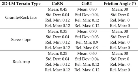
Table 2. Summary of Coefficients of Restitutions (COR) used for the 2D-LM numerical modelling. 2D-LM Terrain Type CoRN CoRT Friction Angle (°)
Granite/Rock face Mean: 0.45 Std Dev: 0.04 Rel. Min: 0.12 Rel. Max: 0.12 Mean: 0.80 Std Dev: 0.04 Rel. Min: 0.12 Rel. Max: 0.12 Mean: 30 Std Dev: 0 Rel. Min: 0 Rel. Max: 0 Scree slope Mean: 0.35 Std Dev: 0.04 Rel. Min: 0.12 Rel. Max: 0.12 Mean: 0.70 Std Dev: 0.03 Rel. Min: 0.9 Rel. Max: 0.9 Mean: 30 Std Dev: 0 Rel. Min: 0 Rel. Max: 0 Rock trap Mean: 0.25 Std Dev: 0.04 Rel. Min: 0.12 Rel. Max: 0.12 Mean: 0.60 Std Dev: 0.04 Rel. Min: 0.12 Rel. Max: 0.12 Mean: 30 Std Dev: 0 Rel. Min: 0 Rel. Max: 0
Table 3. Summary of the rock classes defined for the 2D-LM numerical modelling. 2D-LM Rock Block Classes Mass (kg) Density (kg/m3)
Small Mean: 300 Std Dev: 25 Rel. Min: 75 Rel. Max: 75 Mean: 2650 Std Dev: 10 Rel. Min: 30 Rel. Max: 30 Medium Mean: 1500 Std Dev: 50 Rel. Min: 150 Rel. Max: 150 Mean: 2650 Std Dev: 10 Rel. Min: 30 Rel. Max: 30 Large Mean: 0.25 Std Dev: 0.04 Rel. Min: 0.12 Rel. Max: 0.12 Mean: 0.60 Std Dev: 0.04 Rel. Min: 0.12 Rel. Max: 0.12
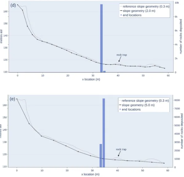
The results of the 2D-LM rockfall analysis are shown in Figure 9. At the scale of this study, a relationship is observed between the geometrical resolution of the DEM and the distribution of rock paths end locations. The behaviour of the simulation, in terms of distribution of rock path end locations is influenced by the DEM resolution. In Figure 9c–e, showing 1, 2 and 5 m slope resolution, respectively, the results highlight uniform distributions, not consistent with the rock debris that can be observed in aerial pictures. As the DEM geometrical resolution increases up to 0.5 and 0.3 m (Figure 9a,b), the end locations distribution becomes more widespread along the slope and representative of the landslide body, as can be observed in Figure 1b. The visual comparison indicates how the majority of the smaller rock fragments are resting in the scree/transition zone mid-slope, and just the larger blocks reach the ditch at the base of the slope.
Figure 9. Results of the Rocfall 2D-LM. The plots show the distribution of end locations along the cross-section. The geometrical resolution adopted for each simulation run is as follows: (a) 0.3 m, (b) 0.5 m, (c) 1 m, (d) 2 m, (e) 5 m.
3.3. 3D Rockfall Trajectory Analysis (Rockyfor3D 3D-RB)
Rockyfor3D was used in order to assess the impact of a rockfall in three dimensions, rather than consider rockfall on a discrete 2D cross section of the slope. 3D analysis would also provide an insight into lateral dispersion of the rockfall deposit when propagating down the slope. The purpose of such simulation was to provide a spatial map of the distribution of end points of rock blocks trajectories, for a specific hazard scenario. The different scenarios were hypothesised based on the understanding of the rock mass conditions, obtained through the geo-mechanical analysis, as well as from screening historical aerial pictures and a geotechnical hazard assessment performed in the field with the help on the mining operation’s personnel. The results are presented in the form of two GIS layers (i.e., reach probability and number of blocks deposited), that once combined, offer a statistically robust way to map the rockfall hazard to be used for risk assessment purposes. The validation phase was achieved through mapping end locations from previous events and comparing this with the results obtained from the simulation. This allows the user to calibrate the model against known end locations and their spatial distribution. The locations of release points were selected by applying an algorithm described in ARPA (2008) [48], which is based on the slope value (expressed in degrees) of each of the DEM’s pixels. The algorithm sets a lower threshold depending on the DEM geometrical
resolution; every pixel in the DEM having a value exceeding that threshold is identified as a candidate release cell. After identification of the potential source locations, all the candidate pixels positions were screened and comparing pixel positions to aerial pictures. Where vegetation cover was present, the potential for release points was discounted. However, where the pixels coincided with exposed bare rock, they were included in the final selection as source areas or release points. As a result of running the ARPA’s algorithm, 48 release points/seeders/pixels were extracted and used as the initial position for rock blocks in the 1 m resolution DEM (17 in the 2 m DEM and six in the 5 m DEM). For cell sizes smaller than 1 m the software reaches its computational limits and cannot compute any trajectory, hence those DEM having a resolution below 1 m were discarded. During each simulation run, selected as a combination of the DEM resolution (5, 2 and 1 m) and rock block classes (small, medium and large), a total of 10,000 block trajectories were simulated. The rock blocks volume, size and shape were set by extracting geometrical characteristics from the TLS/SfM point cloud (Figures 3 and 4). The initial velocity of falling blocks was simulated using a vertical freefall of 4 m (as can be observed in the annotated point cloud image in Figure 3, where the average vertical drop, from the height of the rockfall scars to the bottom of the vertical rock face is about 4–6 m). The COR values, summarised in Table 4, were attached to the raster layers by mapping areas of similar geotechnical properties within GIS. The maximum obstacle height (MOH), expressed as rg70%, rg20% and rg10% was representative of the obstacle height at the slope surface. This represents a statistical distribution of potential obstacles classes, whose values were determined by visual inspection of the slope.
Table 4. Summary of input parameters used for the three-dimensional rigid-body impact model (3D-RB) numerical modelling.
3D-RB
Terrain Type Rockyfor3D Soil Type
Mean CoRN CoRN Value Range Rg70 (m) Rg20 (m) Rg10 (m) Vegetated slope
1—Fine soil material (depth >
~100 cm) 0.23 0.21–0.25 0.3 0.5 0.9
Scree slope
4—Talus slope (Ø > ~10 cm), or compact soil with large
rock fragments
0.38 0.34–0.42 0.25 0.5 0.9
Rock trap 1—Fine soil material (depth >
~100 cm) 0.23 0.21–0.25 0.01 0.05 0.15
Haul road
5—Bedrock with thin weathered material or soil
cover
0.43 0.39–0.47 0 0 0.1
The CORT is derived from this map through an implicit calculation of the software based on the statistical distribution of MOH values [47]. Figures 10–12 show the results of the simulations undertaken. These show the probability of a block to be arrested in a given cell of the DEM (reach probability) and the total number of blocks end location per pixel (number of blocks deposited). The simulations were run on DEM with different resolutions, namely 5 m (Figure 10), 2 m (Figure 11), and 1 m (Figure 12) and using the three rock classes, small, medium and large (Table 5), to observe the effect of the geometrical resolution of the DEM on modelled results, and the ability to capture fine scale irregularities within the topography.
Table 5. Summary of the rock classes defined for the 3D-RB numerical modelling.
3D-RB Rock Classes Volume (m3) Block Shape (m) Density (kg/m3) Mass (kg)
Small 0.125 Cubic 0.50 × 0.50 × 0.50 2650 331
Medium 0.576 Cubic 0.80 × 0.80 × 0.90 2650 1526
Medium 0.576 Rectangular 0.40 × 0.80 × 1.80 2650 1526
Figure 10. Rockyfor3D results computed on the 5 m resolution DEM. Left hand images (a,c,e) show the reach probability layers, on the right (b,d,f) the number of rocks deposited. The first row shows (a,b) results obtained with the rock class ‘SMALL’, second row (c,d) with ‘MEDIUM’ and the third row (e,f) with ‘LARGE’. Rock block classes’ properties are summarised in Table 5.
Figure 11. Rockyfor3D results computed on the 2 m resolution DEM. Left hand images (a,c,e) show the reach probability layers, on the right (b,d,f) the number of rocks deposited. The first row shows (a,b) results obtained with the rock class ‘SMALL’, second row (c,d) with ‘MEDIUM’ and the third row (e,f) with ‘LARGE’. Rock block classes’ properties are summarised in Table 5.
Figure 12. Rockyfor3D results computed on the 1 m resolution DEM. Left hand images (a,c,e) show the reach probability layers, on the right (b,d,f) the number of rocks deposited. The first row shows (a,b) results obtained with the rock class ‘SMALL’, second row (c,d) with ‘MEDIUM’ and the third row (e,f) with ‘LARGE’. Rock block classes’ properties are summarised in Table 5.
As part of the 3D modelling investigation, another variable was introduced: the rock block shape. Figure 13 shows the difference in terms of lateral spread and runout distance of blocks having the same volume and mass but a different shape, cubic in panel (a) and rectangular in panel (b). The increased reach of asymmetrical elongated blocks emerges for every topography resolution adopted.
Figure 13. Comparison of reach probability layers showing the effect of block shape; panel (a) shows the runout of equidimensional (cubic) blocks, while panel (b) shows the runout of elongated (rectangular) blocks. Rock block classes’ properties are summarised in Table 5.
4. Discussion
The results obtained from the rockfall trajectory analysis have provided insights into the behaviour of the rockfall event(s), while exploring the effectiveness of remotely sensed data (ALS, TLS and SfM derived point clouds) as basis for creating DEM for numerical modelling. The reach probability maps and the distribution of end points obtained with both the 2D-LM and 3D-RB approaches showed how there is a positive correlation between the resolution of the DEM and the simulated trajectories. Higher resolution DEM are capable of capturing small scale irregularities, resulting in an increased variability of the end locations. DEM up to 1 m GSD were obtained from
ALS surveys, while very high resolution DEM (GSD ≤ 1 m) were obtained from either TLS or images
acquired with a UAV. The moderate resolution DEM, when implemented in the simulations, gave rise to slower and less energetic trajectories. This analysis would suggest the controlling influence of slope resolution geometry on modelled rockfall end point location.
It is known that large roll out distances are possible when a falling rock’s translational momentum is changed into rotational momentum by impacting the slope, and that launch features may change a rock’s vertical drop to horizontal displacement [49,4]. This analysis confirms that back analysis of rockfall events provide an opportunity to investigate the impact of the geometrical parameters influencing the roll out distance and the distribution of rock paths end locations. The 3D analyses show an acceptable visual correlation between the geometry of the landslide body and the reach probability maps obtained, both in terms of the spread and runout, as shown in Figure 12c–f. The 3D simulation was able to effectively capture the observed typical rockfall trajectory and lateral extent of the resultant rockfall debris.
The 3D modelling has highlighted the impact of the Maximum Obstacle Height (MOH) on results. It is therefore important to undertake sensitivity analyses on this key input parameter during back analyses and establish statistically robust distributions in 3D-RB rockfall simulation using RF3D. The study has highlighted that, where possible, it is important to include field mapping to provide rigorous validation of data. Results from modelling undertaken on this case study demonstrate the
dilemma in rockfall simulation. Unrealistic results are obtained where the surface topography included in the model is too coarse; unrealistic behaviour of modelled rockfall trajectories can also arise when inappropriate COR are used as inputs. From the analyses undertaken there is an inability of the three-dimensional model to correctly simulate observed rockfall trajectories for high resolution DEM which results from poor fine scale mapping, used to associate input parameters to the digital topography, and results in poor zonation of end locations. Dorren (2004) [50] suggests the use of DEM ranging from 25 to 2 m, for regional scale and slope scale simulations. This case study has highlighted considerable variance in rockfall trajectory when increasing the DEM resolution, up until reaching the computational limits of the software and CPU. It is important therefore to calibrate rock block classes, COR, and MOH classes and include a topography of a specific resolution that enables a robust representation of specific scenario being modelled. The resolution achieved with both TLS and SfM is considerably greater than the one selected to generate DEM at the grid sizes used in this study, so it appears that the computational power/hardware requirements/algorithms remain the main obstacle to the use of sub-metric DEM. It is important to acknowledge the impact of DEM on modelled results and the need for guidelines to target optimal resolutions when generating DEM to be used for rockfall trajectory analyses.
As part of the modelling undertaken, another key aspect was the definition of the rock-trap geometry used within the models. The barrier in place to restrict the horizontal travel distance of rock blocks is a critical part of the rock-trap system. However, given its geometry (i.e., an embankment, usually made of sand or crushed rocks), the inner side of the embankment is occluded from a position external to the rock-trap itself, such as the haul road. This condition is usually overcome by capturing the scene from a mobile platform, such as a UAV. The ALS derived model proved to be useful when used in numerical modelling, provided they did not include any region of occlusion. The steepness of the rock wall represents an unfavourable condition that can be addressed by ALS with due precautions (i.e., a careful flight plan design, so to avoid occlusions while capturing the scene), but this is not often feasible, as for this study the ALS dataset was obtained without this specific need in mind, resulting in some data useless for the purpose of numerical modelling. TLS derived models were also ineffective as they were unable to image the inner zone of the rock-trap. From Figure 14 it appears that, regardless of the RS technique used, the 1 m resolution DEM represents the maximum threshold necessary for obtaining an optimal description of the rock-trap geometry.
Figure 14. Comparison of vertical profiles, extracted from the DEM at different resolutions. The vertical axis is exaggerated by a factor of two.
From the analyses undertaken, the shape of blocks modelled also has a significant influence on the rockfall simulation results. In the 3D-RB approach, the medium rectangular class appears to reach further distances compared to equidimensional (cubic) blocks having same mass and volume, going against the general understanding that larger mass and inertia will lead to a longer runout. Although it is not clear what mechanism adopted in the models could lead to such an outcome, the main hypothesis is that elongated blocks tend to roll perpendicular to their major axis, hence gaining high angular momentum compared to the equidimensional blocks. This increased angular velocity is directly linked to a greater horizontal travel distance for rock fragments.
The results show the importance of undertaking both two-dimensional and three-dimensional modelling for the case study, but emphasis is given for the need of both calibration and validation of results to ensure confidence for future use in hazard and risk evaluation.
5. Conclusions
The case study highlights how 3D photogrammetric remotely sensed data can be effectively used to inform the back analysis of a rockfall event at slope scale. The topographic reconstruction of the 3D scene was obtained by using different remote mapping techniques which included aerial and terrestrial laser scanning, and image acquisition by UAV. The resultant high resolution point clouds were then analysed by extracting geo-mechanical features to characterise the rockmass. This included definition of the orientation and spatial distribution of discontinuities within the rock slope. The discontinuity data was subsequently used to perform kinematic admissibility analysis to highlight the potential for both direct and oblique toppling from the columnar jointing. The point cloud data was also used to establish in-situ block size and rockfall block size distribution from the rockfall debris for input data and validation respectively.
Analysis of a series of aerial images was used to determine evolution phases of the rockfall and establish the size and spatial distribution of rock blocks resting on the slope (end point locations). Geo-mechanical and geotechnical features were then translated into modelling parameters, to allow a probabilistic, process-based rockfall trajectory analysis to be performed using both two- and three-dimensional approaches.
The results of the three-dimensional modelling show how the modelling can realistically capture rockfall trajectories in terms of spatial distribution and runout pathways. The models were able to demonstrate the effectiveness of the existing rock-trap. However, the results show the importance and need for calibration of input parameters, as modelled results are clearly influenced by the resolution of the surface topography used within the models. Validation of models through comparison with end point locations is therefore essential for confidence in future use of such models for hazard and risk assessment. The results of the analysis would suggest that guidelines are necessary when using remote mapping data for generation of surface topography for rockfall trajectory analysis, as the spatial resolution of the surface topography has a critical influence on the modelled behaviour. Guidelines are therefore needed to establish suitable DEM resolutions for generation of surface topographies that enable realistic rockfall simulation.
The ability to assess the rockfall behaviour in both two and three dimensions greatly improves the understanding of hazards posed to the mining operation. The methodology proposed within this study can provide the basis for calibration of rockfall input parameters relevant to the case study site and therefore provide the framework for future rockfall hazard assessment and evaluation. This will then provide the basis for risk assessment and design of suitable protection measures.
Author Contributions: Investigation, Carlo Robiati, Matt Eyre, Mirko Francioni, John Coggan and Adam Venn; Formal Analysis, Carlo Robiati, Matt Eyre and John Coggan; Data Curation, Carlo Robiati, Matt Eyre and John Coggan; Methodology and Validation, Carlo Robiati, Matt Eyre, Mirko Francioni and John Coggan; Supervision, Mat Eyre and John Coggan; Writing-original draft, Carlo Robiati; Writing-review and editing, Carlo Robiati, Matt Eyre, Claudio Vanneschi, Mirko Francioni and John Coggan.
Funding: This research received no external funding.
References
1. Riquelme,A.;Cano,M.;Tomás,R.;Abellán,A.IdentificationofRockSlopeDiscontinuitySetsfromLaser ScannerandPhotogrammetricPointClouds:AComparativeAnalysis. Procedia Eng. 2017, 191,838–845. doi:10.1016/j.proeng.2017.05.251.
2. Health and Safety at Quarries. Quarries Regulations 1999. Approved Code of Practice and Guidance; L118 (Second edition); Health and Safety Executive: 2013.
3. Hutchinson,J.N.GeneralReport:Morphologicalandgeotechnicalparametersoflandslidesinrelationto geologyandhydrogeology.In Proceedings of the Fifth International Symposium on Landslides, Lausanne, Switzerland, 10–15 July 1988;Bonnard,C.,Ed.;Balkema:Rotterdam,TheNetherlands,1988;Volume1,pp. 3–35.
4. Ritchie,A.M. Evaluation of Rockfall and Its Control;WashingtonStateHighwayCommission.Committeeon LandslideInvestigations:1961.
5. Varnes,D.J.SlopeMovements.TypesandProcesses.TRBSpecialReport176.In Landslides: Analysis and Control;TransportationResearchBoard, Washington D.C.:1978;pp.11–33.
6. Cruden,D.M.;Varnes,D.J. Landslide Types and Processes; SpecialReport;TransportationResearchBoard, U.S.NationalAcademyofSciences, Washington DC: 1996;247, p. 36–75.
7. McCauley, M.L.; Works, C.B.W.; Naramore, S.A. Rockfall Mitigation; California Department of
TransportationReport:Sacramento,CA,USA,1985.
8. Wyllie,D.C.;Mah,C.W. Rock Slope Engineering: Civil and Mining,4thed.;Routledge:2004;p.456.
9. Chau,K.T.;Wong,R.H.C.;Lee,C.F.RockfallProblemsinHongKongandSomeNewExperimentalResults for Coefficients of Restitution. Int. J. Rock Mech. Min. Sci. 1998, 35, 662–663. doi:10.1016/S0148-9062(98)00023-0.
10. Chau,K.T.;Wong,R.H.C.;Wu,J.J.Coefficientofrestitutionandrotationalmotionsofrockfallimpacts. Int. J. Rock Mech. Min. Sci. 2002, 39,69–77.doi:10.1016/S1365-1609(02)00016-3.
11. Crosta,G.B.;Agliardi,F.Amethodologyforphysicallybasedrockfallhazardassessment. Nat. Hazards Earth Syst. Sci. 2003, 3,407–422.doi:10.5194/nhess-3-407-2003.
12. Dorren,L.K.A.Areviewofrockfallmechanicsandmodellingapproaches. Prog. Phys. Geogr. 2003, 27,69– 87.doi:10.1191/0309133303pp359ra.
13. Alejano,L.;Veiga,M.;Gómez-Márquez,I.;Dellero,H.Applicationofrockfallriskassessmenttechniques intwoaggregatequarries.In Harmonising Rock Engineering and the Environment;Zhou,Y.,Ed.;CRCPress, Florida:2011;pp.1861–1864.ISBN978-0-415-80444-8.
14. Corominas,J.;Matas,G.;Ruiz-Carulla,R.Quantitativeanalysisofriskfromfragmentalrockfalls. Landslides
2019, 16, 5–21.doi:10.1007/s10346-018-1087-9.
15. Jaboyedoff,M.;Dudt,J.P.;Labiouse,V.Anattempttorefinerockfallhazardzoningbasedonthekinetic energy,frequencyandfragmentationdegree. Nat. Hazards Earth Syst. Sci. 2005, 5,621–632.
16. Salvini,R.;Francioni,M.;Riccucci,S.;Bonciani,F.;Callegari,I.Photogrammetryandlaserscanningfor analysing slopestability androck fallrunoutalong the Domodossola-Isellerailway, theItalianAlps.
Geomorphology 2013, 185,110–122.
17. Abellán,A.;Vilaplana,J.M.;Martínez,J.Applicationofalong-rangeTerrestrialLaserScannertoadetailed
rockfall study at Vall de Núria (Eastern Pyrenees, Spain). Eng. Geol. 2006, 88, 136–148.
doi:10.1016/j.enggeo.2006.09.012.
18. Francioni,M.;Stead,D.;Clague,J.J.;Westin,A.Identificationandanalysis oflargepaleo-landslidesat MountBurnaby,BritishColumbia. Environ. Eng. Geosci. 2018, 24,221–235.
19. Francioni,M.;Coggan,J.;Eyre,M.;Stead,D.Acombinedfield/remotesensingapproachforcharacterizing landslideriskincoastalareas. Int. J. Appl. Earth Obs. Geoinf. 2018, 67,79–95.
20. Jaboyedoff,M.;Oppikofer,T.;Abellán,A.;Derron,M.-H.;Loye,A.;Metzger,R.;Pedrazzini,A.Useof LIDARinlandslideinvestigations:Areview. Nat. Hazards 2012, 61,5–28.doi:10.1007/s11069-010-9634-2. 21. Lato,M.J.;Vöge,M.Automatedmappingofrockdiscontinuitiesin3Dlidarandphotogrammetrymodels.
Int. J. Rock Mech. Min. Sci. 2012, 54,150–158.doi:10.1016/j.ijrmms.2012.06.003.
22. Riquelme,A.;Cano,M.;Tomás,R.;Abellán,A.IdentificationofRockSlopeDiscontinuitySetsfromLaser ScannerandPhotogrammetricPointClouds:AComparativeAnalysis. Procedia Eng. 2017, 191,838–845. doi:10.1016/j.proeng.2017.05.251.
23. Fukuzono,T.Anewmethodforpredictingthefailuretimeofaslope.InProceedingsof4thInternational ConferenceandFieldWorkshoponLandslides,Tokyo,Japan, 23-31 August,1985;pp.145–150.
24. Hutchinson,D.J.;Lato,M.;Gauthier,D.;Kromer,R.;Ondercin,M.;vanVeen,M.;Harrap,R.Applications ofremotesensingtechniquestomanagingrockslopeinstabilityrisk.InProceedingsoftheGeoQuebec 2015,QuebecCity, QC, Canada, September 20-23,2015; p. 11.
25. Martino,S.;Mazzanti,P.Integratinggeomechanicalsurveysandremotesensingforseacliffslopestability analysis:TheMt.Puccicasestudy(Italy). Nat. Hazards Earth Syst. Sci. 2014, 14,831–848. doi:10.5194/nhess-14-831-2014.
26. Salvini,R.;Francioni,M.;Riccucci,S.;Fantozzi,P.L.;Bonciani,F.;Mancini,S.Stabilityanalysisof“Grotta delleFelci”Cliff(CapriIsland,Italy):Structural,engineering–geological,photogrammetricsurveysand laserscanning. Bull. Eng. Geol. Environ. 2011, 70,549–557.doi:10.1007/s10064-011-0350-2.
27. Tonini,M.;Abellan,A.RockfalldetectionfromterrestrialLiDARpointclouds:Aclusteringapproachusing R. J. Spat. Inf. Sci. 2014, 8,95–110.doi:10.5311/JOSIS.2014.8.123.
28. Carrivick,J.L.;Smith,M.V.;Quincey,D.J. Structure from Motion in the Geosciences;WileyBlackwell, New York:2016;p. 210.
29. Francioni,M.;Salvini,R.;Stead,D.;Coggan,J.Improvementsintheintegrationofremotesensingandrock slopemodelling. Nat. Hazards 2018, 90,975–1004.doi:10.1007/s11069-017-3116-8.
30. Giordan,D.;Hayakawa,Y.;Nex,F.;Remondino,F.;Tarolli,P.Reviewarticle:Theuseofremotelypiloted aircraftsystems(RPASs)fornaturalhazardsmonitoringandmanagement. Nat. Hazards Earth Syst. Sci.
2018, 18,1079–1096.doi:10.5194/nhess-18-1079-2018.
31. Salvini,R.;Mastrorocco,G.;Esposito,G.;DiBartolo,S.;Coggan,J.;Vanneschi,C.Useofaremotelypiloted aircraftsystemforhazardassessmentinarockyminingarea(Lucca,Italy). Nat. Hazards Earth Syst. Sci.
2018, 18,287–302.doi:10.5194/nhess-18-287-2018.
32. Ellis,R.J.;Scott,P.W.Evaluationofhyperspectralremotesensingasameansofenvironmentalmonitoring in the St. AustellChina clay (kaolin)region, Cornwall, UK. Remote Sens. Environ. 2004, 93, 118–130. doi:10.1016/j.rse.2004.07.004.
33. Hill,P.I.;Howe,J.H.PrimarylithologicalvariationinthekaolinizedStAustellGranite,Cornwall,England.
J. Geol. Soc. 1996, 153,827–838.doi:10.1144/gsjgs.153.6.0827.
34. Tannant,D.ReviewofPhotogrammetry-BasedTechniquesforCharacterizationandHazardAssessment
ofRockFaces. Int. J. Geohazards Environ. 2015, 1,76–87.doi:10.15273/ijge.2015.02.009.
35. Sturzenegger,M.;Stead,D.Quantifyingdiscontinuityorientationandpersistenceonhighmountainrock slopesandlargelandslidesusingterrestrialremotesensingtechniques. Nat. Hazards Earth Syst. Sci. 2009,
9,267–287.doi:10.5194/nhess-9-267-2009.
36. Markland,J.T. A Useful Technique for Estimating the Stability of Rock Slopes when the Rigid Wedge Slide Type of Failure is Expected; Rockmechanics research report;report no. 19; Interdepartmental RockMechanics Project,ImperialCollegeofScienceandTechnology, London:1972.
37. Turner,A.K.;Duffy,J.D.ModellingandpredictionofRockfalls.In Rockfall: Characterization and Control; TRB:2012, Washington D.C.
38. Dorren,L.K.A.Areviewofrockfallmechanicsandmodellingapproaches. Prog. Phys. Geogr. 2003, 27,69– 87.doi:10.1191/0309133303pp359ra.
39. Li,L.;Lan,H.Probabilisticmodellingofrockfalltrajectories:Areview. Bull. Eng. Geol. Environ. 2015, 74, 1163–1176.doi:10.1007/s10064-015-0718-9.
40. Asteriou,P.;Saroglou,H.;Tsiambaos,G.Geotechnicalandkinematicparametersaffectingthecoefficients ofrestitutionforrockfallanalysis. Int. J. Rock Mech. Min. Sci. 2012, 54,103–113.
41. Chau,K.T.;Wong,R.H.C.;Wu,J.J.Coefficientofrestitutionandrotationalmotionsofrockfallimpacts. Int. J. Rock Mech. Min. Sci. 2002, 39,69–77.doi:10.1016/S1365-1609(02)00016-3.
42. Bar,N.;Nicoll,S.;Pothitos,F.Rockfalltrajectoryfieldtesting,modelsimulationsandconsiderationsfor steep slope design in hard rock. In Proceedings of the First Asia Pacific Slope Stability in Mining Conference,BrisbaneCity,Australia,6–8September,2016;p.10.
43. Azzoni, A.; Rossi, P.P.; Drigo, E.; Giani, G.P.; Zaninetti, A. In situ observation of rockfall analysis parameters.InProceedingsoftheVIInternationalSymposiumonLandslides,Christchurch,SouthIsland, NewZealand,10–14February1992.
44. Bourrier,F.;Berger,F.;Tardif,P.;Dorren,L.;Hungr,O.Rockfallrebound:Comparisonofdetailedfield experimentsandalternativemodellingapproaches. Earth Surf. Process. Landf. 2012, 37,656–665.
45. Spadari,M.;Giacomini,A.;Buzzi,O.;Fityus,S.;Giani,G.P.InsiturockfalltestinginNewSouthWales, Australia. Int. J. Rock Mech. Min. Sci. 2012, 49,84–93.doi:10.1016/j.ijrmms.2011.11.013.
46. Stevens,W.D.ROCFALL:AToolforProbabilisticAnalysis,DesignofRemedialMeasuresandPrediction ofRockfalls.Master’sThesis,UniversityofToronto,Toronto,ON,Canada,1988.
47. Dorren,L.K.A. Rockyfor3D v5.2 revealed. In Transparent Description of the Complete 3D Rockfall Model.ecorisQ paper; ecorisQ:Geneva,Switzerland,2016;p.32.
48. Arpa Piemonte—Centro Regionale perle Ricerche Territoriali eGeologiche. In ARPA Progetto n. 165 PROVIALP, Protezione Della Viabilità Alpine—Relazione Finale;Arpa Piemonte, Italy:2008.
49. Pierson, L.A.;Gullixson,C.F.;Chassie,R.G. Rockfall Catchment Area Design Guide;Final Report(Metric Edition).OregonDepartmentofTransportationandFederalHighwayAdministration:2001.
50. Dorren,L.K.A.;Maier,B.;Putters,U.S.;Seijmonsbergen,A.C.Combiningfieldandmodellingtechniques toassessrockfalldynamicsonaprotectionforesthillslopeintheEuropeanAlps. Geomorphology 2004, 57, 151–167.doi:10.1016/S0169-555X(03)00100-4.
51. CloudCompare™.Availableonline:https://www.danielgm.net/cc/(accessedon March 2018). 52. Rocfall™.Availableonline:https://www.rocscience.com/software/rocfall(accessedon February 2019). 53. Rockyfor3D™.Availableonline:http://www.ecorisq.org/ecorisq-tools(accessedon February 2019). 54. RocscienceDIPS™.Availableonline:https://www.rocscience.com/software/dips(accessedon March 2018). 55. ArcGIS™.Availableonline:http://desktop.arcgis.com/en/arcmap/(accessedon July 2019).
56. AutoCAD™. Available online: https://www.autodesk.com/products/autocad/overview (accessed on
March 2018).
©2019 by the authors. Licensee MDPI, Basel, Switzerland. This article is an open access article distributed under the terms and conditions of the Creative Commons Attribution (CC BY) license (http://creativecommons.org/licenses/by/4.0/).