RESEARCH PAPER
Multi-temporal land use classification using hybrid
approach
Lakshmi N. Kantakumar
a,*, Priti Neelamsetti
ba
Institute of Environment Education and Research, Bharati Vidyapeeth University, Pune, India b
JV Analytical Services, Bopodi, Pune, India
Received 10 June 2015; revised 28 August 2015; accepted 7 September 2015 Available online 28 September 2015
KEYWORDS
Multi-temporal land use; Hybrid classification; Decision trees; Threshold technique; India
Abstract Land use and land cover (LULC) classification of a satellite image is one of the prereq-uisites and plays an indispensable role in many land use inventories and environmental modeling. Many studies viz., forest inventories, hydrology and biodiversity studies, etc., are in demand to account the dynamics of land use and phenology of vegetation. Multi-temporal land use classifica-tion accounts the phenology of vegetaclassifica-tion and land use dynamics of the study area. In this study, a hybrid classification scheme was developed to prepare a multi-temporal land use classification data set of Sawantwadi taluka of Maharashtra state in India. Parametric classification methods like max-imum likelihood and ISODATA clustering methods are combined with the non-parametric decision tree approach to generate the multi-temporal LULC dataset. The accuracy assessment results have shown very promising results with a 93% overall accuracy with a kappa of 0.92.
Ó2015 Authority for Remote Sensing and Space Sciences. Production and hosting by Elsevier B.V. This is an open access article under the CC BY-NC-ND license (http://creativecommons.org/licenses/by-nc-nd/ 4.0/).
1. Introduction
Classification is a process of segregating the information or data into a useful form. Classification of satellite imagery is based on placing pixels with similar values into groups and identifying the common characteristics of the items repre-sented by these pixels (Purkis and Klemas, 2011). Hence, a cor-rectly classified image will represent areas on the ground that share particular characteristics as specified in the classification
scheme (Lillesand et al., 2008). The land use and land cover inventories are very important for many planning and manage-ment activities. Remote sensing data is a primary source and used extensively for land use classification. The LULC classifi-cation process itself tends to be subjective and in fact, there is no logical reason to expect that one detailed inventory should be adequate for more than a short time, since land use and land cover patterns change in keeping with demands for natu-ral resources (Anderson, 1976). In practice, sevenatu-ral land use and land cover classification (LULC) techniques/algorithms are available, viz., supervised, unsupervised, decision tree or knowledge based, object oriented, artificial neural network and support vector machines classification techniques. How-ever, no one ideal classification technique/algorithm exists and is unlikely that one could ever be developed (Anderson, 1976). Multi-temporal land use classification accounts the * Corresponding author at: Institute of Environment Education &
Research, Bharati Vidyapeeth University, Pune-Satra Road, Pune 411043, India. Tel.: +91 20 24375684; fax: +91 20 24362155.
E-mail address:[email protected](L.N. Kantakumar). URL:http://ieer.bharatividyapeeth.edu(L.N. Kantakumar). Peer review under responsibility of National Authority for Remote Sensing and Space Sciences.
H O S T E D BY
National Authority for Remote Sensing and Space Sciences
The Egyptian Journal of Remote Sensing and Space
Sciences
www.elsevier.com/locate/ejrswww.sciencedirect.com
http://dx.doi.org/10.1016/j.ejrs.2015.09.003
1110-9823Ó2015 Authority for Remote Sensing and Space Sciences. Production and hosting by Elsevier B.V. This is an open access article under the CC BY-NC-ND license (http://creativecommons.org/licenses/by-nc-nd/4.0/).
seasonal variation of the study area, such as seasonal vegeta-tion differences, which is very useful to understand the impact of land use dynamic on the natural resources (Wolter et al., 1995). In the present study, a hybrid approach has been designed in combination of maximum likelihood supervised classification technique, decision tree approach and unsuper-vised classification method to derive the multi-temporal land use classification of Sawantwadi taluka for the year 2013. The Landsat-8 imageries belonging to dry and wet seasons are used to account the phenological changes of the vegetation in the study area over a year.
2. Study area
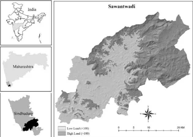
Sawantwadi taluka (Fig. 1) of Sindhudurg district is located at the South West corner of the Maharashtra state of India. The study area is bounded between 15° 430–16° 30 latitudes in northern hemisphere and 73° 410–74° 50 longitudes lies east of Greenwich. The study area is known for wooden crafts and a major tourist attraction in Maharashtra. The study area elevation ranges from 1 m to 1029 m above sea level. It can be divided into two parts based on the topography, a low-lying flat terrain in western region and elevated, undulating terrain in eastern region of the study area. The low-lying region is mainly dominated by agriculture, mango gardens and built-up land uses, whereas the forest and shrub land cover domi-nates the high-lying region.
3. Datasets
For multi-temporal land use and land Cover (LULC) classifi-cation Landsat-8’s April 2013 (dry period) and December 2013 (wet period) terrain corrected level 1 data were obtained from the public domain service of USGS EROS data center, Sioux Falls, USA. ASTER GDEM is a product of METI and NASA has been used as a reference vertical surface throughout the study. Open Map Series (OSM) toposheets of 1:50,000 scale surveyed in the year of 2005 have been collected from the Sur-vey of India and rectified to the WGS84 datum and further projected on UTM-43 north zone based on WGS84. The toposheet mosaic is used as ancillary data at the time of super-vised classification and for assessment of accuracy. ENVI 5.3 is used for the image processing purpose in the study.
4. Methodology
A satellite image of one point in time does not incorporate the sufficient information about the phenology of the vegetation and the temporal characteristics of land use classes. A mini-mum of two satellite images at different points in time (In gen-eral, dry and wet periods) over a year are required to address the temporal characteristics of land use features. Since multi-temporal classification involves two or more images, it is always advisable to carry out the atmospheric correction to the satellite imageries (Coppin et al., 2004). MODTRAN4
Figure 1 Study area map with elevation showing geographic location of Sawantwadi taluka (elevation source: ASTER GDEM version 2, METI of Japan and NASA).
based FLAASH module is used to carry out the atmospheric corrections of the study area. The atmospherically corrected imageries further processed by using hybrid classification approach are as described in the flow chart (Fig. 2).
4.1. Atmospheric corrections
Earth atmosphere consists of a mixture of gases, liquid and solid particles, most of these are optically active causing absorption, diffusion and scattering. Signal measured at the satellite is the emergent radiation from the Earth surface– atmosphere system in the sensor observation direction (Camps and Camps-Valls, 2011). The radiance measured at sensor is known as Top of Atmosphere (TOA) radiance (Chander et al., 2009), atmospheric corrections aim to convert
the TOA radiance of the objects into the near earth reflectance. In this study, MODTRAN4 based FLAASH module in ENVI 5.3 was applied to carry out the atmospheric corrections of the satellite images. FLAASH is an acronym of Fast Line of sight Atmospheric Analysis of Spectral Hyper cubes with a capabil-ity of correcting the wavelengths in the visible through near-infrared and shortwave infrared regions, up to 3lm. It includes correction for the adjacency effect, cirrus and opaque cloud classification and adjustable spectral polishing for arti-fact suppression. FLAASH provides additional flexibility when compared to the other widely used atmospheric correc-tion programs, i.e., Atmospheric REMoval program (ATREM), Atmospheric CORrection Now (ACORN), it allows custom radiative transfer calculations for a wider range of conditions including off-nadir viewing and all MODTRAN
Toposheet Field Data Wet Period Dry Period Refined Dry ML image
Georeferenced Satellite Image
Atmospheric correction
Atmospherically corrected Image
Training Sites Max. Likelihood Classification Maximum Likelihood (ML) classification output Threshold Decision tree False Color Composite Visual Interpretati Multi-Temporal Dataset Decision Tress Rules Refined Wet ML image Apply Pixels with Rules YES NO Pixels with No Rules Masked Multi-Temporal Dataset with no rule pixels No Rules Mask Multi-Temporal Dataset Classified image (Pixels with no rules) Multi-Temporal Image with one
forest class Forest Mask Masked Multi-Temporal Dataset with Forest Pixels ISODATA Clustering Classified image with different forest type Multi-Temporal Image
standard aerosol models (Kruse, 2004). Tropical atmosphere module, maritime aerosol model with 2-Band (K–T) aerosol retrieval method has been used to perform the atmospheric corrections of the study area satellite images. The 2-Band (K–T) aerosol retrial method uses the initial visibility value if the aerosol cannot be retrieved.Fig. 3shows the spectral pro-files of a forest pixel located at 15°550 3500N and 73°580 3000E before and after atmospheric correction in both wet and dry seasons.
4.2. Multi-temporal classification
A hybrid approach combines maximum likelihood supervised, decision tree and ISODATA clustering technique has been applied to prepare the multi-temporal classified image. Firstly, maximum likelihood supervised classification approach is used to classify the atmospherically corrected individual satellite images to map the land use classes of a particular point (dry and wet periods) in time. The outputs further are refined and are combined by using knowledge based decision tree approach into a multi-temporal classified image. An unsuper-vised classification approach further applied to identify various forest cover types.
4.2.1. Maximum likelihood classification
Supervised classification requires the analyst to select training samples from the data which represents the themes to be clas-sified (Jensen, 1996). The training sites are geographical areas previously identified using ground-truth to represent a specific thematic class (Purkis and Klemas, 2011). Then the statistics of the Digital Number (DN) associated with the training sites are used to classify each pixel in the satellite imagery into the cor-responding LULC classes. Several algorithms of supervised approach are available viz., Parallelepiped, Minimum Distance to Mean (MDM), maximum likelihood (ML), Mahalanobis Distance, The Jeffries–Matusita (J–M) Distance, Linear Discriminant Analysis, Spectral Angular Mapping (SAM) and Spectral Information Divergence (SID). In this study, widely used maximum likelihood classification technique is adopted for LULC classification.
The main advantage of the maximum likelihood classifier is, it not only considers the mean vector of the pixels in one
class, but also takes into account the spread or variability of these pixels in multispectral feature space. The maximum like-lihood classification assumes that the statistics for each class in each band are normally distributed and calculates the proba-bility that a given pixel belongs to a specific class (Jensen, 1996). Unless a probability threshold is selected, all pixels will be classified and each pixel is assigned to the class that has the highest probability (Lein, 2011).
As a first step in the supervised classification, one should select the training sites. In this study the training sites are selected based on the field sampling data done during Nov– Dec 2013, Survey of India toposheets and visual interpretation techniques. The dry and wet period datasets are separately classified into ten land use classes i.e., water, built-up, agricul-ture, plantation, stone quarry, fallow land, grass land, open and dense shrub land, and forest.
4.2.2. Decision tree approach
Decision tree approach is very useful, when it is difficult or insufficient to recognize thematic classes based on spectral characteristics of remote sensing data (Coppin et al., 2004). Decision trees have several advantages for remote sensing applications by virtue of their relatively simple, explicit, and intuitive classification structure (Friedl and Brodley, 1997) and can be used for both classification and post classification refinement. Further, decision tree algorithms are strictly non-parametric and, therefore, make no assumptions regarding the distribution of input data, and are flexible and robust with respect to nonlinear and noisy relations among input features and class labels (Friedl and Brodley, 1997).
Knowledge or decision is introduced by a set of rules:ifa condition exists,theninference is applied, especially this is very useful in multi temporal land use classification (Konecny, 2003). Some of the forest pixels on hill slopes were misclassified as agriculture land use during the maximum likelihood classi-fication. The agricultural land in the study area is located along the streams and in the flat terrain. Therefore, the mis-classification error of forest to agriculture was rectified by applying a knowledge based decision rule, i.e., the agricultural pixels having degree slope greater than 10 have been converted into forest land cover before applying multi-temporal decision rules. Table 1shows the accuracy assessment results of land
Figure 3 Spectral profiles of a forest pixel located at 15°550 3500N and 73° 580 3000E (a) before atmospheric corrections (b) after atmospheric corrections.
use classifications pertaining to both dry and wet seasons. The results are showing the classification scheme performed better in wet season than in dry season.
In order to combine the individual land use classifications into a single multi-temporal land use image i.e., the represen-tation of a whole year a multi temporal classification schema based on decision tree rules has been applied (Wagner et al., 2013). A hierarchy of the land cover classes based on pheno-logical characteristics has been formed to derive the rules for multi-temporal classification. In the natural land classes the hierarchy is as follows, i.e., forest, shrub, open shrub and grassland. The main assumption made in the multi-temporal classification scheme is the later land class will be updated into the immediate higher category, if there is a potential conflict existing between the two classes in both dry and wet seasons. For example, if a pixel is classified as forest in one season and shrub land in other season, it will be assigned to forest in the multi-temporal classification. Similarly, if a pixel is clas-sified as agriculture in one season and either plantation or bar-ren land in other season, it will be assigned to agriculture class. Table 2shows the applied rules to combine the dry and wet seasons land use maps into a single multi-temporal land use image.
4.2.3. Unsupervised classification
Unsupervised classification procedure needs no prior knowl-edge of the study area. This method is objective and entirely data driven. Even for a well-mapped area, unsupervised classi-fication may reveal some spectral features which were not apparent beforehand (Liu and Mason, 2009). In this study, ISODATA clustering technique was adopted to distinguish the different forest covers types. ISODATA algorithm calcu-lates class means evenly distributed in the data space then iter-atively clusters the remaining pixels using minimum distance techniques (Melesse and Jordan, 2002). Each iteration recalcu-lates means and reclassifies pixels with respect to the new means. This process continues until the number of pixels in each class changes by less than the selected pixel change threshold or the maximum number of iterations is reached. The forest cover in the decision tree output after applying the multi-temporal rules is used as a mask on both dry and wet period scenes to segregate the forest cover into 15 different clusters. The 15 different classes were further analyzed and
combined into 4 forest classes namely evergreen forest, semi-evergreen forest, moist-deciduous forest and mixed jungle based on the ground truth data collected during the field visit in Nov–Dec 2013 and by using visual interpretation techniques and expert knowledge about the study area. A 3 * 3 majority analysis window was applied to the output after unsupervised classification to remove misclassified pixels.Fig. 4, shows the final output of the multi-temporal land use/land cover of 2013 of study area.
5. Results and discussion
Accuracy assessment involves the comparison of the catego-rized data to the reference data for the same sites (Jensen, 2007; Lachowski, 1996). The error matrix is the standard way of presenting results of the accuracy assessment (Story and Congalton, 1986). Error matrix is also called as confusion matrix used for characterizing the performance of a classifica-tion technique (Rees, 1999). Overall accuracy is one of the common measure of classification accuracy and is the ratio of sum of the diagonal entries (also called thetrace) to the total number of pixels examined, which gives the proportion of sam-ples that have been correctly classified (Campbell and Wynne, 2011). Kappa coefficient can be used as another measure of agreement or accuracy and allows to test whether an individual land-cover map generated from remotely sensed data is signif-icantly better than a map generated by randomly assigning labels to areas (Lunetta and Lyon, 2004).
In this study, ground truth ROIs have been used to assess the accuracy of the multi-temporal LULC image produced after majority analysis. A 33 majority analysis window removes misclassified and spatially singular pixels within homogeneous areas (Wagner et al., 2011). Field data, Survey of India toposheets and Google Earth were used to develop the ground truth data. The overall accuracy of the 2013 multi-temporal image was recorded as 93% (Table 3). In the multi-temporal image 13% of evergreen forest was wrongly classified as semi-evergreen forest and 13% of the plantation
Table 1 Accuracy assessment results of individual land use classification pertaining to dry and wet seasons.
Period Dry Wet
Overall accuracy 84.54% 91.10%
Kappa coefficient 0.81 0.89
Class User acc. (percent) User acc. (percent)
Water 100 99.58
Stone quarry/sand 65.79 66
Forest 95.59 97.6
Open shrub land 78.48 95.18
Grass land 21.18 37.45
Barren land/fallow land 92.26 97.35
Agriculture 39.43 95.67
Plantation 100 75.28
Built-up 59.68 50.56
Shrub land 84.48 91.91
Table 2 Rules used to derive a multi-temporal land use
classification.
Class combinations Multi-temporal result Forest–shrub land Forest
Forest–grass land Shrub land Shrub land–grass
land
Open shrub land Shrub land–open
shrub land
Shrub land Open shrub land–
grass land
Open shrub land Grass land–barren land Grass land Agriculture–barren land Agriculture Plantation– agriculture Agriculture Equal land use in two
scenes
Equal land use
No rules apply New classification using both dry and wet period scenes
wrongly attributed as moist deciduous forest and 6% open shrub land misclassified as barren/fallow land. The mixed jun-gle class was recorded with less accuracy at about 70%, this value was reasonable because mixed jungle class is a mixture of all forest classes.
The Kappa coefficient of the 2013 multi-temporal classified image which is above 0.92 indicates that the classification method very well captured the dynamics of the land use and
land cover of the area of interest in that particular study year (Alexakis et al., 2012; Lunetta and Lyon, 2004).
6. Conclusion
The classification of remote sensing data is subjective and mainly depends on the purpose of the study. The multi-temporal land use classification accounts the phenology of the vegetation and dynamics of the land use. It is often used as input data in many environmental modeling, hydrological and biodiversity assessment studies. The hybrid classification approach developed in this study is a combination of paramet-ric and non-parametparamet-ric approaches, hence very useful to develop the multi-temporal land use datasets by taking the advantages in both the approaches. The developed approach includes the post-classification refinement by using threshold based knowledge approach, which is helpful to rectify the com-mon misclassification errors. The decision tree approach used to produce the multi-temporal land use data is strictly non-parametric and based on the expert knowledge, therefore very subjective in nature. The accuracy assessment results are very promising and encouraging for the developed approach. The results showing, the developed approach captured the impervi-ous land use classes viz., built-up and stone quarries with user accuracy not less than 96%. The developed classification schema is very successful in discriminating the natural vegetation with accuracy not less than 75%, because natural vegetation classes overlap each other on feature space and hard to discriminate.
Figure 4 Multi-temporal land use 2013 of the Sawantwadi taluka.
Table 3 Producers and User accuracies of each land use/cover of multi-temporal land use classification of 2013.
Overall accuracy 93.22% Kappa coefficient 0.9225
Class Prod. acc. (percent) User acc. (percent)
Water 100 100
Stone quarry/sand 99.2 96.88
Evergreen forest 86.52 78.97
Open shrub land 94.27 100
Grass land 100 99.32
Barren land/fallow land 100 91.03
Agriculture 99.09 97.32
Plantation 84.57 92.75
Built-up 100 96.3
Shrub land 99.47 75.2
Semi evergreen forest 95.43 86.52 Moist deciduous forest 90.91 90.16
Acknowledgments
The authors are thankful to Dr. C. P. Vibhuthe, Mr. Yogesh Mendhe, Mrs. Anuja Karhu of YIC, Bopodi, Pune for their necessary support. We greatly acknowledge Landsat data from EROS data center, USGS, Sioux Falls. ASTER GDEM ver-sion 2 data from Ministry of Economy, Trade and Industry (METI) of Japan and NASA.
References
Alexakis, D.D., Agapiou, A., Hadjimitsis, D.G., Retalis, A., 2012. Optimizing statistical classification accuracy of satellite remotely sensed imagery for supporting fast flood hydrological analysis. Acta Geophys. 60, 959–984. http://dx.doi.org/10.2478/s11600-012-0025-9.
Anderson, J.R., 1976. A Land Use and Land Cover Classification System for Use with Remote Sensor Data. U.S. Government Printing Office.
Campbell, J.B., Wynne, R.H., 2011. Introduction to Remote Sensing, Fifth ed. Guilford Press.
Camps, G., Camps-Valls, G., 2011. Remote Sensing Image Process-ing. Morgan & Claypool Publishers.
Chander, G., Markham, B.L., Helder, D.L., 2009. Summary of current radiometric calibration coefficients for Landsat MSS, TM, ETM+, and EO-1 ALI sensors. Remote Sens. Environ. 113, 893– 903.http://dx.doi.org/10.1016/j.rse.2009.01.007.
Coppin, P., Jonckheere, I., Nackaerts, K., Muys, B., Lambin, E., 2004. Digital change detection methods in ecosystem monitoring: a review. Int. J. Remote Sens. 25, 1565–1596. http://dx.doi.org/ 10.1080/0143116031000101675.
Friedl, M.A., Brodley, C.E., 1997. Decision tree classification of land cover from remotely sensed data. Remote Sens. Environ. 61, 399– 409.http://dx.doi.org/10.1016/S0034-4257(97)00049-7.
Jensen, J.R., 2007. Remote Sensing of the Environment: An Earth Resource Perspective. Pearson Prentice Hall.
Jensen, J.R., 1996. Introductory Digital Image Processing: A Remote Sensing Perspective. Prentice Hall.
Konecny, G., 2003. Geoinformation: Remote Sensing, Photogramme-try and Geographic Information Systems. Taylor & Francis. Kruse A.F., 2004. Comparison of ATREM, ACORN, and FLAASH
atmospheric corrections using low-altitude AVIRIS data of Boul-der. Presented at the JPL Airborne Geoscience Workshop, CA: Jet Propulsion Laboratory, Pasadena.
Lachowski, H., 1996. Guidelines for the Use of Digital. DIANE Publishing.
Lein, J.K., 2011. Environmental Sensing: Analytical Techniques for Earth Observation. Springer Science & Business Media.
Lillesand, T.M., Kiefer, R.W., Chipman, J.W., 2008. Remote Sensing and Image Interpretation. John Wiley & Sons.
Liu, J.G., Mason, P., 2009. Essential Image Processing and GIS for Remote Sensing. John Wiley & Sons.
Lunetta, R.S., Lyon, J.G., 2004. Remote Sensing and GIS Accuracy Assessment. CRC Press.
Melesse, A.M., Jordan, J.D., 2002. A comparison of fuzzy vs. augmented-ISODATA classification algorithms for cloud-shadow discrimination from Landsat images. Photogramm. Eng. Remote Sens. 68, 905–912.
Purkis, S.J., Klemas, V.V., 2011. Remote Sensing and Global Environmental Change. John Wiley & Sons.
Rees, G., 1999. The Remote Sensing Data Book. Cambridge Univer-sity Press.
Story, M., Congalton, R., 1986. Accuracy assessment – A user’s perspective. Photogramm. Eng. Remote Sens. 52, 397–399.
Wagner, P.D., Kumar, S., Fiener, P., Schneider, K., 2011. Hydrolog-ical modeling with SWAT in a monsoon-driven environment: experience from the Western Ghats, India. Trans. ASABE 54, 1783–1790.
Wagner, P.D., Kumar, S., Schneider, K., 2013. An assessment of land use change impacts on the water resources of the Mula and Mutha rivers catchment upstream of Pune, India. Hydrol. Earth Syst. Sci. Discuss. 10, 1943–1985. http://dx.doi.org/10.5194/hessd-10-1943-2013.
Wolter, P.T., Mladenoff, D.J., Host, G.E., Crow, T.R., 1995. Improved forest classification in the northern Lake states using multi-temporal Landsat imagery. Photogramm. Eng. Remote Sens. 61, 1129–1144.