Signal analysis tool to investigate walking abnormalities

(1)

FACULTY OF INFORMATION TECHNOLOGY AND ELECTRICAL ENGINEERING

Seyed Amir Mirmojarabian

Signal Analysis Tool to

Investigate Walking Abnormalities

Master’s Thesis

Degree Program in Biomedical Engineering

June 2018

(2)

thesis, 51 p.

ABSTRACT

This thesis presents a signal analysis tool, which has been designed to investigate walking abnormalities which are related to foot rolling movements during walk-ing; interaction of foot with ground which is called stance phase. They would cause a wide range of severe anatomical damages such as ankle, leg, heel and back pain in the long-term.

Comparing to the conventional data acquisition setups of biomechanical re-searches, inertial measurement sensors (IMU), which are being used widely as an appropriate alternative setup recently, facilitate monitoring human movement for a long-term period out of laboratory. This justifies the growing trend of improv-ing the IMU-based algorithms which are designed for events detection, position calculation, and rotation estimation. Therefore, a set of 4 IMUs, placed on shank and foot of both legs, has been used for data collection.

In data processing stage, two novel algorithms have been developed and imple-mented as the backbone of the designed software aiming to detect and integrate stance phases. The first algorithm was developed to detect stance phases in gait cycle data. Even though the detection of events in gait cycles has been the topic of a majority of biomechanical researches, stance phase as the interval between two consecutive events has not been studied sufficiently. The second algorithm, sensor alignment, generates a rotation matrix which is used to align IMU sensors placed on the same foot and shank. This alignment of the two sensors enables us to add or subtract the data point-wisely to make a more meaningful interpretation of the data regarding thought-out walking abnormalities during phase stances.

The visualized results of the thesis can be considered as an early stage of a more comprehensive research which might lead to quantitative results corresponding to different walking abnormalities.

Keywords: Gait event detection and validation, Initial contact, Terminal stance, Gyroscope, and Accelerometer, Sensor alignment, IMU.

(3)

My deep gratitude goes first to my family who supported me throughout my life. Sec-ondly I would also like to express my special thanks of gratitude to my supervisor, Professor Tapio Seppänen. At last, I would like to thanks Mr. Kai Noponen and Dr. Tero Klemola for their valuable advices in the thesis work.

(5)

ABBREVIATIONS

TO Toe-off HS Heel strike MS Mid stance

IMU Inertial Measurement Unit DOF Degree of Freedom

MEMS Micro-electromechanical System EMG Electromyography

SVM Signal Vector Magnitude SVD Singular Value Decomposition

θ(t) Angular Position

˙

θ Angular Velocity

Ts Sampling Period

Ax Anterior Acceleration Signals

Az Superior Acceleration Signals

σ_n2_j Variance

Acc,gStart Gravitational Acceleration

Mag Magnetic Field of Earth Cro Cross Product of Acc and Mag

SF_R _{the orientation of IMU coordinate system (S) to the forearm}

coordinate system (F)

S_xF _{x direction of the forearm frame with respect to IMU}

coor-dinate system

S_yF _{y direction of the forearm frame with respect to IMU}

coor-dinate system

S_zF _{z direction of the forearm frame with respect to IMU}

coordi-nate system

ωP ron angular velocity during rolling foot inward

ωSup angular velocity during rolling foot outward

(SEN iRSEGi) the orientation of the body segment coordinate system with

respect to the coordinate system of the sensor unit

(SEN i

b

xSEGi) x direction of the body segment coordinate system with

re-spect to the coordinate system of the sensor unit

(SEN i

b

ySEGi) y direction of the body segment coordinate system with

(SEN i_bzSEGi) z direction of the body segment coordinate system with

(sω) Angular velocity a quaternion vector S

Eqω,t Orientation of the sensor coordinate system with respect to

(6)

1. INTRODUCTION

1.1. Background & Motivation

A normal person walks 5000-6000 steps in averages daily, even though it is recom-mended to walk 10000 steps per day to keep health benefits. Because of this, it is ob-vious to say that walking is one of the most frequent physical activity which has been the topic of human motion studies for centuries. Without a doubt, Da Vinci (1452-1519) is one of the pioneers whom described human movements. Back to recent days, extraction of temporal parameters of gait cycle has gained a significant attention since it has been used in many medical tools and applications, from clinical diagnostic and medical rehabilitation to everyday life such as preventing elderlies to fall by predic-tion abnormal gait temporal parameters. Tradipredic-tionally, there have been some reliable gait analysis systems like high-speed video recording, pressure mat, footswitches, op-tical capture and GaitRite systems. Even though these gait analysis systems are able to provide high reliable measurement of temporal gait parameters, their usage is only limited to a dedicated laboratory which make them more proper for research purposes. Since the mentioned gait analysis systems are complex, expensive, laborious and time consuming, they are rarely used out of a laboratory. In addition, The main drawback of these systems is the path of walking which is restricted to a laboratory environment. Then it is very difficult to claim that the gathered data is a proper representative of a person gait cycle.

In order to overcome these weaknesses, new technologies has been embedded in small sensors which can be mounted easily on different parts of the body and don’t have previous limitations. IMU1 _{is a general term which refers to these sensors. They}

usually consist of miniaturized accelerometers, gyroscopes, magnetometer, a small digital signal processor, a memory, and a wireless transmitter unit. Digital signals collected by an IMU which have a repeating pattern are called gait; a particular semi-automatic task of a limb which consists of strides and usually is measured from forefoot and shank. A stride is defined as a given point in the repeating gait pattern to the next same point with similar characteristic for that limb.

IMUs usually have triaxial accelerometers, gyroscopes and magnetometers which provide simultaneous measurements in three orthogonal directions and corresponding rotations around the axes. Figure 1 illustrates the accelerometers axes and gyroscope rotations corresponding to the IMU placed on forefoot.

It is usual that accelerometer x-axis is positioned in the anterior-posterior direc-tion, y-axis in the lateral-medial direction and z-axis in the inferior-superior direction. The gyroscope captures rotation within three planes perpendicular to the determined axes; frontal plane (around x-axis), sagittal plane (around y-axis) and transverse plane (around z-axis). According to the reasons above, IMU is a suitable device to study walking abnormalities when a subject is out of a lab doing daily activities.

In order to have a precise comprehension of walking abnormalities related to foot rolling movements during stance phase, it is necessary to identify key movement (ro-tation) of the ankle joint complex; plantar/dorsiflexion, occurring in the sagittal plane;

(7)

6

ab/adduction occurring in the transverse plane and inversion/eversion, occurring in the frontal plane, see figure 2, [1].

Figure 1. (a) Accelerometer directions, (b) Gyroscope Rotations.

Figure 2. Diagram illustrating relative motions of the ankle joint complex. Figure adapted from Visual 3D. [1]

If the walking abnormalities are to be studied, it is necessary to distinguish stance phase intervals since it is the interaction of foot with ground causing them. Hence, the purpose of this thesis is to present a novel signal analysis tool to investigate the walking abnormalities related to foot rolling movements after extracting stance phase durations.

(8)

2. MEASUREMENT OF MOTION USING IMU

In this chapter the principles, operation procedure and application details of IMU in motion estimation and attitude calculation are presented. We will then, review the measurement principle of an IMU, an accelerometer and a gyroscope. Finally, the faulty behavior and errors of gyroscopes and magnetometers will be discussed.

2.1. Inertial Measurement Units

An inertial sensor (IMU) consists of multi-axis sensors; accelerometers, gyroscopes and magnetometers sensors. The accelerometer is used to measure the inertial accel-eration, whereas angular rate is recorded by gyroscope. On the other hand, magne-tometer measures the magnetic field vector which can be used to adjust the gyroscope data in order to avoid drift issue. Nevertheless, magnetometer is highly prone to be af-fected by external magnetic field. Every sensor typically has three degree of freedom to measure three-dimensional local coordinate system leading to the total of 9 DOF. An appropriate calibration is required before alignment of orthonormal base represented by local coordinate system of a sensor with outer casing of the sensor. Having a reli-able estimation of orientation and position of an object, it is recommended to initialize measurement with alignment procedure providing that IMU is rigidly attached to an object [2, 3].

Inertial sensors have been primarily employed in major industries like aviation since they were massive in size, costly and insufficient in terms of power consumption. How-ever, significant development in microelectromechanical system (MEMS) has been the reason for novel development of IMU sensors contributing to smaller, lighter and low cost sensors. Because of this, the lately enhanced IMUs are being broadly utilized across various application domains ranging from industry quality control and medical rehabilitation to robotics and navigation system. The common medical applications are expressed in Table 1. Type I and Type II in IMU type are categorized as IMU with two types of sensors and three types of sensors respectively [2].

Table 1. Applications in medical rehabilitation [2]

Device/Usage IMU Type Fusion Method Exoskeleton for Rehabilitation Type II Mirror therapy concept Exoskeleton for Rehabilitation Type II EMG

Post-Stroke Rehabilitation Monitor Type II None Post-stroke arm rehabilitation Type II None Arm posture correction Type II Unknown Post-traumatic movement analysis Type I None

Last but not least, regarding a reasonable IMU determination for a particular ap-plication, it is prescribed to consider some essential criteria like package size, data accuracy, saturation level, sampling frequency, response rate and degree of freedom which might differ case by case [2].

(9)

8

2.2. MEMS Accelerometer

The working principle of a typical MEMS accelerometer is established on a mechan-ical suspension system which is composed of two sets of plates; one set is fixed to a solid ground plane on a reference frame and the other set is attached to a proof mass mounted on spring designed to reflect mechanical displacement of the elastic spring in response to an applied acceleration, as shown in figure 3. The variation of capacitance between the fixed and moving plates corresponds to applied acceleration. The deflec-tion of proof mass is measured using the capacitance difference since the free-space (air) capacitances between the movable plate and stationary outer plates are functions of the corresponding displacements. Hence, components of acceleration are measured from the displacement caused either due to the effect of gravity or the other corre-sponds to the motion of sensor [3, 4, 5].

Figure 3. The structure of a MEMS accelerometer [5].

2.3. MEMS Gyroscope

A gyroscope is any device which measures angular velocity or maintain orientation based on the principles of the conservation of momentum. There are 4 main types of gyroscopes with respect to operational mode; spinning, optical, vibratory, NMR. MEMS gyroscopes are classified into the vibratory type with a wide range of applica-tions for different purposes as mentioned in below [4, 6].

• Automotive for Reliability; Promoting anti-skid control,

• Industrial for Robustness; Precision machinery, Antenna stabilization,

• Consumer side for compact size and low prize; Gaming, Health and fitness, Optical Image Stabilization, Pedestrian Navigation,

One of the most extensively used MEMS gyroscopes is the tuning fork composed of a structure fixed at the anchors and large movable proof masses on either sides (fig-ure 4). The struct(fig-ure resonates at one of its natural frequencies. When the struct(fig-ure

(10)

begins to rotate, the Coriolis force causes a force perpendicular to the proof masses of the fork detected as bending of the tuning fork. These forces are proportional to the applied angular rate, from which the displacements can be measured in a capaci-tive mode. Electrostatic, electromagnetic, or piezoelectric mechanisms can be used to detect the force [7, 8].

Figure 4. Gyroscope Mechanical Structure [6].

2.4. Gyroscope Drift and Magnetometer Distortion

Basically, a gyroscope captures angular velocity or the rate of change of the angu-lar position over time deg/s. In other word, the gyroscope data is the derivative of the angular position over time. Therefore, angular position can be simply derived by integration of angular velocity for any particular moment with following equations [9]:

˙ θ = dθ dt (1) θ(t) = Z t 0 ˙ θ dt (2)

On the other hand, due to approximation (sampling) in digital systems, it is not possible to perform an ideal continuous integration; as a result, a finite number of samples taken at a specific sampling period, (Ts), are summed up to make angular

position at a specific time [9].

θ(t)≈ t X 0 ˙ θ(t)Ts (3)

(11)

10 This approximation brings forward errors in particular when frequency components of gyroscope data are higher than sampling frequency. In this case, gyroscope records changes in its position which are faster than sampling frequency and cannot be ex-tracted properly. This error is known as drift because of its aggregation over time (fig-ure 5). Therefore, a gyroscope doesn’t experience the same position after a periodic movement [9, 10].

Figure 5. Integration result of gyroscope signal with different level drift [11]. There are various solutions to tackle the drift issue. Perhaps the most obvious one is to select sampling frequency carefully. It is recommended to choose a sampling frequency of 100Hzfor mechanical systems. However, fusion algorithms like Kalman

filter, complementary filter or gradient descent algorithm are being widely used to compensate the drift issue by using accelerometer or magnetometer data [12, 13].

Towards the end, it has been demonstrated that metal sources existed within the buildings, electrical appliances, metal furniture and metal structures have a destructive effect on magnetometers data leading to magnetic distortion of IMU. Estimation of IMU orientation is highly prone to errors when it is posed to environments contami-nated by metal sources. Magnetic interference can be removed either by calibration or considering additional reference data of orientation such as accelerometer data which is useful to compensate inclination error for the measured earth’s magnetic field [13].

(12)

3. IMU SIGNAL PROCESSING METHODS IN GAIT

ANALYSIS

Detection of temporal gait parameters is the basis of many IMU applications like es-timation of stride length, heading direction and sensor orientation which can be done either by accelerometer or gyroscope signals. The mechanism of gait cycle detection and segmentation methods are usually categorized into three main groups[14]:

1. Searching a specific event in a fixed window, 2. Targeting an event based on its identification, 3. Probing an event in a stationary frame.

The main objective of this chapter is to review stride event detection within both domain of acceleration and angular velocity. Afterward, sensor alignment procedure is explained as it is the essential operation before orientation estimation which is ex-pressed in last section of the chapter.

3.1. Key Points of a Gait Cycle

In general a stride of gait cycle can be categorized into eight events which are repeating in a specific order [14]. Figure 6 shows all the eight events and their corresponding percentage regarding their corresponding time of occurrence in a gait cycle. A gait cycle is usually considered as a stride which begins with ‘initial contact’ when a foot strikes the ground. Initial contact matches to a significant alteration in acceleration, local maximum tracked by dampened vibration in anterior direction. While rotation in sagittal plane shows a local minimum. Stand phase of a gait cycle starts with initial contact and ends with terminal stance which has similar characteristic to initial contact. By finishing the stand phase, a sharp peak in acceleration and a local minimum in angular velocity scope disclose terminal stance. Even though variation of acceleration in initial contact is more dramatic, terminal stance depicts a deeper minimum compared to initial contact in angular velocity. Due to apparent characteristic of the two events, initial contact and terminal stance either in acceleration or angular velocity domains, they are being widely used as two key points in detection algorithms, [14, 15, 16, 17, 18, 19, 20, 21].

(13)

12

Figure 6. Events of a stride [22].

(14)

3.2. Gait Events detection by Accelerometer Signals 3.2.1. Variance/Local extrema of Manipulated Signals

Feature space mapping is an efficient method to highlight events of interest and filter irrelevant data. Two orthogonal acceleration signals, anterior (Ax) and superior (Az),

are used to generate a set of new signals; power, product, and sumsignals, by using basic math operations, see equation (4). [15, 16, 17]

power =A2_x+A2_z , product=Ax×Az , sum =Ax+Az (4)

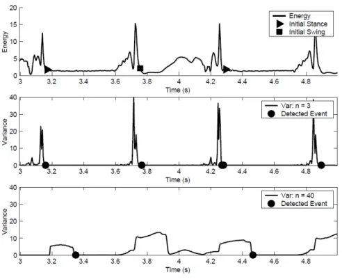
Even though events of interest can be detected by setting simple threshold on ma-nipulated signals, false events detection is likely to occur due to noise. Therefore, it is useful to consider variance, equation (5), as a robust variable showing dynamics of signals, while it is insensitive to bias and temperature drift. There are some events in gait cycle corresponding to abrupt changes in acceleration like initial contact and ter-minal stance, so threshold detection using the variance of power signal can detect the events more reliably, as shown in figure 8. The variance of power signal is commonly calculated over a sliding window with different lengths, see equation (5); a window with smaller length depicts sharper changes [15, 16, 17].

σ2_n j = 1 n i=j+(n−1) X i=j (xi−xi)2 (5)

On the other hand, once the variance has been calculated regardless of the sample size, it is possible to use local extrema to identify different events [15]. As events occur in a determined order in a normal gait cycle, it is usually enough to identify the first event accurately by verifying the event condition as well as its neighbors re-garding either variance changes or local extrema [15]. Table 2 depicts the sequence of gait events, 3 manipulated signals and variance/local extrema description as events conditions/properties which can be investigated [15, 16, 17].

In [15], the main assumption is that intervals centered at initial contact have more variation compared to terminal stance intervals; this assumption is satisfied in some cases. However, it is also likely to have an opposite situation. Therefore, the variation of energy signal of a gait cycle might not be increasing consistently, causing detection and segmentation problem (when calculating max and length of segments).

Table 2. Gait Events Detection Sequence [15]

Events %Stride Energy Product Sum A Initial Stance 0 Variance drops Variance drops Not used B Opp. Foot Strike 50 Variance rises Variance rises Not used C Toe Off 60 Sharp max Sharp max Local max D Initial Swing 65 Variance drops Variance drops Local min F Terminal Swing 85 Not used Local min Local min H Foot Strike 95 Sharp max Not used Sharp max

(15)

14

Figure 8. Detecting gait events with variance of power signal for sample size 3, 40. [15]

3.2.2. Signal Vector Magnitude

An appropriate method to cancel the noise effect is to calculate Signal Vector Magni-tude using equation 6. Signal Vector MagniMagni-tude represents total acceleration intensity during the gait cycle featuring periodic events. In [24], the recursive algorithm gets a smoothed Signal Vector Magnitude (SVM) to detect dynamic fragments through the processing chain, while it is used as the backbone of wavelet based algorithm to seg-ment gait cycle in [18].

SV M =qA2

x+A2y+A2z (6)

3.3. Gait Events Detection by Gyroscope Signals

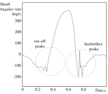
Angular velocity signals of lower limbs are being widely used to extract temporal gait parameters since the rotation around medio-lateral axis of lower limbs shows a precise periodic pattern in sagittal plane [14, 19, 20, 21]. The angular velocity measurements of two different researches have been depicted in figure 9 and 10, showing the same pattern of walking captured in sagittal plane. Regarding low frequency components, a unique pattern can be detected visually in both figures; however, in some moments like initial contact and terminal stance high frequency components make a difference.

(16)

Figure 9. Shank angular velocity showing the presence of peaks during the toe-off and heel strike. [19]

Figure 10. Segmentation algorithm detection for a walking step. [14]

Multi-resolution wavelet decomposition was primary used to determine distinctive signal features of shank angular velocity, initial contact and terminal stance, since wavelets resemble negative peaks of the mentioned events [19]. However, in terms of gait events detection, searching local extrema within angular velocity signal to iden-tify tangible events; initial contact, terminal stance and mid stance, is a widely used methodology. In the following, two different searching algorithms are shown by their flowcharts [14, 20, 21].

(17)

16

Figure 11. Signal segmentation algorithm flow diagram. [14]

The algorithm whose flowchart shown in figure 11 detects consecutive zero cross-ing points indicatcross-ing swcross-ing phases. However, in order to have acknowledged initial contacts (foot strikes), maximum of angular velocity should be greater the particular threshold (1.5 rad/s). In addition, there are 3 experimental conditions which applies to initial contact instances (tmin) and swing phase moments (tmax), which are supposed

(18)

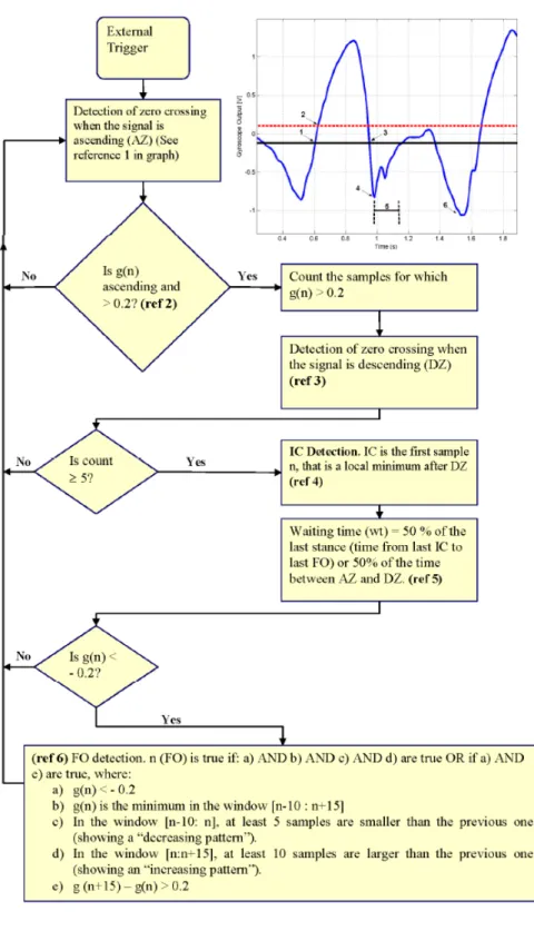
Figure 12. Flowchart of the algorithm used for detection of Initial Contact and Foot Off from the gyroscope signal. [20]

The operation mechanism of the algorithm shown in figure 12 has a high correlation with the one shown in figure 11; initializing with zero crossing detection, and them predetermined experimental conditions are investigated to verify considered events , initial contacts and terminal stances.

(19)

18

3.4. Sensor Alignment

In order to have a better understanding of gait temporal parameters, it is recommended to align IMU sensors which are usually placed on specific body segments; for example, in our case shanks and feet. After alignment procedure, position and orientation of the IMU are estimated with respect to a global frame, as it represents valuable information. If IMU sensors alignment are supposed to be done, it is important to have a clear view on how an orientation of one coordinate system with respect to another coordinate system is obtained.

While IMU placement and the coordinate system definition are usually determined based on the purpose of a research and the device characteristics, there is a norm to compensate the offset between local and global frame which is called "static calibra-tion trial"; backbone of sensor alignment procedures. In general, static calibracalibra-tion trial starts with a stationary subject in a predefined anatomical position doing several pre-defined movement. Then the device deflection in a particular direction is estimated. Finally, a correction factor can be utilized to correct the deflection. In other word, to transfer/represent a measurement captured in a local coordinate system with/into a global coordinate system, the orientation of the local coordinate system with respect to the global coordinate system is required [25, 4]. In the following, two researches of sensor alignment are expressed:

In [25], two IMUs are used, one placed on the dorsal side of the forearm and the other on the lateral side of the upper arm. Forearm alignment procedure requires the orientation of the IMU with respect to the forearm which can be achieved by instructing the subject several predefined movements of forearm,"static calibration trial", shown in figure 13.

(20)

Considering forearm and signals captured in the IMU coordinate system, the orien-tation of IMU coordinate system (S) to the forearm coordinate system (F) is presented by a rotation matrix and consisting of the 3 unit vectors of the forearm.

SF

R= [SxF SyF SzF] (7)

As it can be seen in equation 7, all axes of the IMU, as local coordinate system, can be used to specify the directions of the forearm frame; the relative orientation of two coordinate systems.

• y_axis of the forearm specifies by the direction of the angular velocity either during rolling foot inward(ωP ron)or outward(ωSup),

S yF = ωP ron |ωP ron| =− ωSup |ωSup| (8)

• z_axis of the forearm can be measured by the direction of gravity at the start and end of the trial by accelerometer (The minus sign in the right subscript means that the value will be recalculated later),

S

zF−=− gStart |gStart|

(9)

• x_axis of the forearm can be concluded as a cross product of the two measured vectors in y and z directions , however they are not perfectly orthogonal due to measurement errors; so as a solution, z_axis is recalculate to regain the orthog-onality,(The orientation of IMU with respect to the upper arm can be found by a very similar procedure).

SF

R = [SyF ×SzF− SyF (SyF ×SzF−)×SyF] (10) In [26], the authors proposed a two stage static calibration trial to calculate two orientation matrices(SEN i_R

SEGi), foot(i = 1)and leg(i = 2); describing the

orien-tation of the body segment coordinate system with respect to the coordinate system of the sensor unit attached to it.

First, while the subject is standing, a rotation around the longitudinal axis of the whole body is done, shown in figure 14; both the foot and leg segments around the y_axis are rotated. Variation in the axis of rotation , the y_axis of the segment with respect to the sensor coordinate system(SEN i

b

ySEGi), can be calculated by integration

of the gyroscope signal.

Second, while the subject is seating naturally, figure 15, a knee extension with min-imal displacement of the ankle joint is performed, causing a rotation of foot and leg around the z_axis. Again, the integration of the gyroscope signal is computed to de-termine the axis of rotation, the z_axis of each segment with respect to the sensor coordinate system(SEN i

b

zSEGi).

The x_axis of the each segment is the cross product of the y_axis and z_axis. There-fore, the two orientation matrices (SEN iRSEGi) can be presented by the set of three mentioned column vectors, as shown in below:

SEN i

RSEGi= [SEN ixbSEGi

SEN i

b

(21)

20

Figure 14. Determination of the segment y-axis with respect to the sensor coordinate system. [26]

Figure 15. Determination of the segment z-axis with respect to the sensor coordinate system. [26]

3.5. Orientation Estimation

Accurate estimation of IMU’s orientation is vital in a wide variety of industries, for instance in medical industry to monitor a patient’s activity continuously in applications like human motion analysis, motion tracking and rehabilitation.

Kalman filters have been used as the heart of a majority of orientation-based al-gorithms due to its accuracy and effectiveness. However, they have two drawbacks making them expensive computationally:

• Complicated to implement because of large state vector to linearize the problem,

• Required sampling rate might exceed the bandwidth of data

Even though there have been numerous attempts to use alternative techniques such as fuzzy processing, filtering of frequency domain and complementary filter, to solve

(22)

large computational issues in Kalman filter approaches, the applied techniques are ef-fective under limited operating conditions.

A recently proposed solution is to use quaternions to study the relation between two coordinate systems. A quaternions is a four-dimensional complex number to represent the orientation of one coordinate system with respect to another coordinate system in a three-dimensional space after a rotation of angleθaround a predefined axis. Quater-nions not only deliver low computational load and perform efficiently at small sam-pling rate but also simplify the error correction procedure such as drift cancellation and magnetic distortion compensation. Further more, unlike Euler angle representa-tion, quaternions are not subject to problematic singularities [13].

In [13], a novel orientation algorithm which combines quaternions within an op-timized gradient descent approach is presented. The steps of the algorithm can be summarized as below:

• Angular velocity of a sensor coordinate system aroundx, yandz axes are rear-ranged as a quaternion vector(sω),

sω = [0 ωx ωy ωz] (12)

• The quaternion derivative is calculated as the variation of the reference (Earth) coordinate system with respect to the sensor coordinate system(S

Eq˙),

• Orientation of the sensor coordinate system with respect to the reference co-ordinate system at time t can be computed as a numerical integration of the quaternion derivative. S Eq˙ω,t = 1 2 S Eqˆest,t−1⊗sω (13) S Eqω,t =SE qˆest,t−1+SE q˙ω,t∆t (14)

For any initial measurement of the reference coordinate system, it is not possible to have a particular orientation. In addition, quaternion representation accepts just a unique solution, leading us towards an optimization problem which has been handled by gradient descent algorithm.

(23)

22

4. DEVELOPED METHODS

4.1. Stance Phase Detection

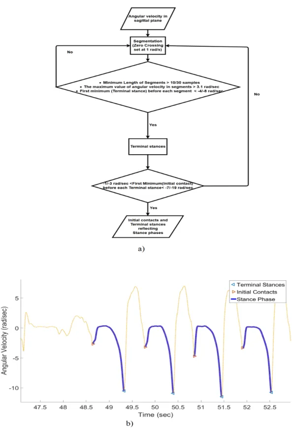
The interaction of foot with ground is called stance phase which begins with initial contact and ends at terminal stance. It is during the stance phase that walking abnor-malities which are related to foot rolling movements of a patient can be captured and modeled. Therefore, the first step of designing a signal analysis tool is to improve an algorithm to detect stance phase durations along with gait cycle trials. As it was men-tioned in 3.3 , angular velocity captured in sagittal plane depicts initial contacts and terminal stances distinctively, making it suitable to be used for gait event detection. However, the diversity of techniques used for detection of these two key events is high. Another dilemma is the definition of a stance phase. Although many algorithms detects initial contacts and terminal stances, the events might not necessary have valu-able information about stance phase. In other word, a given initial contact and terminal stance are likely to represent a particular stance phase unless the distance between them exceed a known threshold which might be happening due to a premature dorsiflexion or plantarflexion when, for example, the subject reduces the speed or turns around.

The proposed algorithm of stance phase detection checks the experimental crite-ria to observe probable initial contacts and terminal stances which represent stance phases. The algorithm begins with a segmentation algorithm which sets a threshold at

1g, gravitational acceleration, to detect the segments which contain mid-stances. The segmentation algorithms is a zero crossing detection algorithm which is set at1g; the beginning of the detected segments happen whenever input angular velocity exceed1g, while segments are terminated when the angular velocity plunge over1g. However, not all the segments lead us towards a stance phase. In order to investigate whether the seg-ments indicate stance phases, an initial contact follows by mid-stance and ends with terminal stance, two sets of conditions are investigated.

The first set determines the possible terminal stances by comparing the length of the segments, maximum of each segment, and the first minimum before each segment with three experimental thresholds.

Then the qualified segments and terminal stances are tested by the second set of con-ditions. A segment and its adjacent terminal stance lead to a stance phase if an initial contact which satisfies the second set of condition is found in a backward interval. The second set of condition is just an experimental interval for the angular velocity signal in sagittal plane when it indicates the initial contact moment. The two sets of condi-tions are given in table 3 and table 4 as well as the algorithm flowchart and definition of stance phase shown in figure 16.

(24)

Figure 16. a) Flowchart of the stance phase detection algorithm, b) Stance phase inter-vals.

(25)

24

Table 3. First Set of Conditions for Stance Phase Detection

Subjects Female Subject Male Subject Minimum Length of Segments 10 Samples > 30 Samples > Maximum value of angular velocity in segments 3rad/s> 3.1rad/s>

First minimum before each segment -4rad/s< -8rad/s< The backward searching interval 30 Samples 30 Samples

Table 4. Second Set of Conditions for Stance Phase Detection Subjects Female Subject Male Subject Initial contact values in the interval -1 to -7rad/s -3 to -19rad/s

The backward searching interval 40 to 80 Samples 90 to 170 Samples

4.2. Sensor Alignment

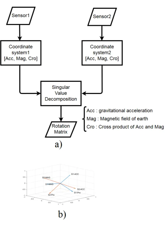
In order to analyze the rotation/relation between sensors and magnify gait cycle events, we aligned the coordinate systems of each two sensors placed on shank and foot which is called sensor alignment algorithm. The first step of the algorithm is to create a par-ticular coordinate system for each sensor with three axes. We have used gravitational acceleration and magnetic field of earth as two main axes. They were measured by each IMU when the subject was standing stationary. The third axis was calculated as cross product of two first axes. As a consequence, we have created a three columns of data shaping a matrix which considered as coordinate system matrix.

After computing the coordinate system matrix for each sensor, we have used singular value decomposition to extract a rotation matrix which represents the rotation/relation between two specific coordinate system matrices; a rotation matrix is a powerful tool enabling us to map one coordinate system matrix to another. The flowchart of the sensor alignment algorithm and coordinate systems of the sensors placed on shank and foot are illustrated in figure 17.

(26)

Figure 17. a) Flowchart of the sensor alignment algorithm, b) Coordinate systems of the two sensors.

(27)

26

4.3. Graphical user interface

In order to make the proposed algorithms more intuitive, a GUI has been designed to be visual interface of the signal analysis tool. The main purposes of the GUI are explained as:

• Showing the different types of data captured by IMUs (Acceleration, angular velocity and magnetic field of earth),

• Showing videos of trials (front view and side view),

• Synchronization of video files and IMU data,

• Scrolling up/down and moving along the data stream to study a targeted events,

• Illustrating the coordinate systems of IMUs,

• Illustrating the total angular velocity of differently placed IMUs (shank and foot) after alignment

• Illustrating the relative angular velocity of differently placed IMUs (shank and foot) after alignment

(28)

Figure 18. Main layout of the GUI

Main layout of the GUI after loading IMUs data and video files, while no activity has been triggered, is shown in figure 18. As it can be seen the layout surface was divided into 3 main areas:

• Displaying Signals: 12 signals of the 4 IMUs (Accelerometer, Gyroscope, Mag-netometer),

• Displaying Videos: 2 videos from 2 different perspectives and scroll bar,

• Displaying buttons.

In this figure, signals and videos have been loaded to the software. The first required activity is to choose the type of input and load the data, videos and synchronization files.

(29)

28

Figure 19. Main layout of the GUI

Initially, there will be just a stationary display of the loaded data and synchronized videos, whereas there are some control buttons such as "Play", "Stop" and "Get Point" enable us to control the display process. The black vertical line is set at the beginning of physical activity (jumping), and it starts moving horizontally during display after pushing the "Play" button. The buttons can be categorized into 3 main groups:

• loading and initial displaying,

• processing and displaying the result,

• Controlling the display.

(30)

Figure 20. Coordinate systems

Once the display has been halted, by pushing the "Stop" button, the processing but-tons are activated which are supposed to apply the two proposed algorithms to the data. "Coordinate Sys" button depicts the calculated coordinate system of sensors in one frame; there is a plot for each leg showing two coordinate systems of the leg. Layouts of coordinate systems are shown in figure 20.

(31)

30

Figure 21. Total angular velocity of differently placed IMUs (shank and foot) after alignment

Another processing button is "Total at Feet". After transferring data captured at a shank to the foot by rotation matrix, the two data sets are added together to generate the total movement data set of the leg (foot) in the 3 planes. Total angular velocities of three different planes, point-wisely added the foot angular velocity and aligned shank angular velocity, are depicted in figure 21.

(32)

Figure 22. Relative angular velocity of differently placed IMUs (shank and foot) after alignment

The last processing button is "Relative at Feet". The aligned shank data to the foot by rotation matrix and the foot data are subtracted to create the relative movement data set of the leg (foot) in the 3 planes. Relative angular velocities of three different planes, point-wisely subtracted the foot angular velocity and aligned shank angular velocity, are depicted in figure 22.

Until resuming the display of data and videos by "Play" button, loading and control-ling buttons are off. However, while the GUI is in the playing mode displaying data and synchronized videos, loading and controlling buttons remain inactive.

(33)

32

5. EXPERIMENTAL RESULTS

5.1. Sensor and Data Information

In total 8 subjects ( 2 females and 6 males ) have participated in the 8 tests held at Oulu Health Labs. Each subject has performed three trials in each test including at least 20 gait cycles in each trial. Throughout trials, four miniature IMU devices were attached to subjects’ lower limbs, one on each shank and one on each forefoot. Each of the de-vices uses two separate chips; 1) Kionix KMX62, triaxial magnetometers, 2) KXG03, triaxial accelerometers and gyroscopes; generating two CSV files, first one containing gyroscope and accelerometer data and the second one containing magnetometer data. Sampling frequency and time stamp coefficient are the same for both files of an IMU; however, the MAC address of sensors are different. One of the IMUs and is depicted in figure 23. The data files were stored on a local server zipped with camera recorded files.

(34)

5.2. High-speed Camera and Activity Protocol

Walking trials were recorded by two high speed camera with 120 frame rate. One camera was positioned in front of the subject, while the other camera recorded the side view. Regarding movement protocol, after an initial pause, the subjects have clapped and jumped. These actions were used for synchronization and alignment of IMU sensors and videos. Next, the subjects have walked at a normal speed in the walking path. In the trials, the walking path consists of 4 sub-paths including at least 5 gait cycles in each. After each sub-path, the subjects have reduced the speed and turned back to start the next sub-path. The fourth path ended at the start point, where the trials were completed by a final pause, see figure( 24, 25) .

Figure 24. Front view of high-speed camera

(35)

34

5.3. Visualization Results

The graphical results of the two proposed algorithms are shown in this section. First, angular velocities of IMUs placed on foot during stance phase are shown, all gyroscope planes. The first trials of test 3 to 8 have been selected to detect stance phases. In each trial, mean and variation around mean of angular velocities in the detected stance phases have been computed and depicted. Then, for each selected trial and each leg, the coordinate systems of IMU placed on shank and foot (before and after alignments) are shown.

5.4. Analysis of the Results

A stance phase interval includes 4 main events: initial contact, loading response, mid-stance and terminal mid-stance [22]. The detected mid-stance phases might have different lengths, either they are from the same trial, different subjects or different genders. Conducting a comparison among stance phases requires all the stance phases to have the same length. Interpolation is the mathematical tool that is used to serve that pur-pose. Interpolated stance phases were generated for the first trial of test3 to test8 shown in figures 26 to 31.

By having the length of stance phases fixed to a particular value (1500 samples), it is possible to determine the corresponding percentage of the 4 events associating in the stance phases. In a simplified form, it can be said that initial contact and loading re-sponse occurs during the first 30 percent of the stance phase (0 to 30%), while terminal stance occupies the last 30 percent (70% to 100%), and mid-stance is the 40 percent of the stance phase left in the middle. Unlike figures pertinent to test 3 and test 4 (figures 26 and 27), abrupt changes in initial contacts, loading responses and terminal stances events can be observed in figures 28 to 31. Therefore, the 3 events and their changes might be appropriate indicators for walking related abnormalities, whereas mid-stance is not likely to carry valuable information.

Another significant perception is the variation of angular velocity signals embedded within stance phases. Even though this might be also an indicator corresponding to walking abnormalities carrying worthwhile information, it might have been caused by some artifacts such as not attaching the IMU sensor firmly to the body segment.

With respect to the IMU alignment algorithm shown in figures 32 to 37, calculated rotation matrices present a numerical criterion to analyze walking related abnormali-ties; however, since rotation matrices are computed during stationary period, rotation matrices should have a dynamic mechanism to update themselves throughout the gait cycle, such as gradient descent algorithm.

(36)

Figure 26. Test3-trial1, angular velocities of IMU placed on foot during stance in 3 planes

(37)

36

(38)

(39)

38

(40)

(41)

40

(42)

Figure 32. Test3-trial1, coordinate systems of IMU placed on shank and foot before and after alignments

(43)

42

(44)

(45)

44

(46)

(47)

46

(48)

6. DISCUSSION

6.1. Detection of stance phase intervals

Detection of gait cycle events is an important step of most locomotion analysis al-gorithms. Different searching and matching algorithms are being used to extract the desired events; wavelet matching algorithm is a well-known example to mention [14, 19, 20, 21]. However, if it is needed to extract a specific interval of gait cy-cles, stance phases, for particular applications such as studying walking abnormalities which are related to foot rolling inwards or outwards during walking, the conventional algorithms are not able to handle the requirement properly as events are detected in-dividually without concerning other events. The main purpose of the proposed stance phase algorithm is to determine and detect two consecutive events which represent acceptable stance phases. This purpose has been fulfilled by considering two sets of conditions for the consecutive events. Only if the paired-events could reach the deter-mined conditions, the intervals between them are considered as stance phases; other-wise, they are rejected. To makes it more clear, two different cases are given in which the paired-events are not the representative of stance phases; 1) When a subject jumps, 2) When the subject’s foot touches the ground very smoothly.

6.2. Alignment of Sensors

The main motivation behind the proposed alignment algorithm is to study the relation of the sensors placed on one leg, shank and foot. The relative motion of the two sensors is more meaningful in terms of embedded pattern of the walking abnormalities. The basis of the alignment algorithm is to compute the rotation matrix used for mapping coordinate systems.

6.3. Future Work

Verification of the proposed algorithms is the first step which needs to be taken for further improvement; an alternative source of data (true data) extracted from some sort of pressure sensor or slow motion camera should be considered as a gold standard algorithm for verification. The initial setup of the gold standard algorithm should be determined carefully so that the synchronization of the proposed algorithm and the selected gold standard algorithm can be achieved accurately. The correlation of the two algorithms provides a scientific criterion representing the accuracy of the proposed algorithms. Development of optimized data mapping algorithms to use smart phones/ smart watches data as training sets for deep neural networks to estimate the level of the walking abnormalities can be another important step. After designing a deep neural network, it should be trained with transformed data sets collected from rather healthy people by smart wearable devices. it is, then possible to use the design deep neural network for compensation of abnormalities in patients who are suffering, for example, from rolling excessively foot inwards or outwards. In other word, a robotic leg with the embedded deep neural network can imitated the locomotion of a healthy leg.

(49)

48

7. SUMMARY

In this thesis, we proposed two new algorithms to detect and integrate the stance phase intervals of the gait cycles reflecting walking abnormalities which are related to foot rolling inwards or outwards during walking. We have implemented the algorithms into a graphical user interface software which can be used as a signal analysis tool used for diagnostic and rehabilitation purposes. The visualized results (figures) of the algorithms after applying to the data gathered at Oulu Health Labs show promising diagnostic information about the walking abnormalities related to foot movements that should be diagnosed as soon as possible; otherwise, they might cause serious anatom-ical injuries. Therefore, the signal analysis tool can play a vital role to fulfill an early stage diagnosis regarding the considered walking abnormalities; which is totally vi-sually and easy to use. However, to have an improved standard tool, there are some issues, for example verification of the algorithms, which are needed to be handled.

(50)

8. REFERENCES

[1] Brockett C.L. & Chapman G.J. (2016) Biomechanics of the ankle. Orthop Trauma 30, pp. 232–238. URL:http://www.ncbi.nlm.nih.gov/pmc/ articles/PMC4994968/, s1877-1327(16)30048-3[PII].

[2] Ahmad N., Raja Ghazilla R.A., Khairi N. & Kasi V. (2013) Reviews on various inertial measurement unit (imu) sensor applications 1, pp. 256–262.

[3] Seel T. (2016) Learning control and inertial realtime gait analysis in biomed-ical applications: improving diagnosis and treatment by automatic adaption and feedback control. URL: https://books.google.fi/books?id= Dx9wAQAACAAJ.

[4] Valencia L.S.V. (2015) Sensor-to-body calibration procedure and definition of anatomical references for gait analysis based on inertial sensors. Master’s thesis, Federal University of Espírito Santo, http://portais4.ufes.br/posgrad/teses/. [5] Khenkin A. (2009), Sonic nirvana: Mems accelerometers as acoustic

pickups in musical instruments. URL: https://www.sensorsmag. com/embedded/sonic-nirvana-mems-accelerometers-as-acoustic-pickups-musical-instruments.

[6] Mems tuning fork gyroscope. URL: http://dasp.mem.odu.edu:8080/ ~tfork_sp11/theory.html.

[7] Burg A., Meruani A., Sandheinrich B. & Wickmann M. (accessed: 8.1.2018), Mems gyroscopes and their applications. URL: http://clifton.mech. northwestern.edu/~me381/project/done/Gyroscope.pdf. [8] Serrano D. (accessed: 8.1.2018), Design and analysis of mems

gyro-scopes. URL: http://ieee-sensors2013.org/sites/ieee-sensors2013.org/files/Serrano_Slides_Gyros2.pdf.

[9] de Maele P.J.V. (2013), Getting the angular position from gyroscope data. URL:

http://www.pieter-jan.com/node/7.

[10] Hundza S.R., Hook W.R., Harris C.R., Mahajan S.V., Leslie P.A., Spani C.A., Spalteholz L.G., Birch B.J., Commandeur D.T. & Livingston N.J. (2014) Accu-rate and reliable gait cycle detection in parkinson’s disease. IEEE Transactions on Neural Systems and Rehabilitation Engineering 22, pp. 127–137.

[11] Zhong Q. (2016) Development and experimental evaluation of a state-dependent coefficient based state estimator for functional electri-cal stimulation-elicited tasks. Master’s thesis, University of Virginia, https://www.researchgate.net/publication/.

[12] de Maele P.J.V. (2013), Reading a imu without kalman: The complementary filter. URL:http://www.pieter-jan.com/node/11.

(51)

50

[13] Madgwick S.O.H., Harrison A.J.L. & Vaidyanathan R. (2011) Estimation of imu and marg orientation using a gradient descent algorithm. In: 2011 IEEE Interna-tional Conference on Rehabilitation Robotics, pp. 1–7.

[14] Fida B., Bernabucci I., Bibbo D., Conforto S. & Schmid M. (2015) Pre-processing effect on the accuracy of event-based activity segmentation and clas-sification through inertial sensors. Sensors 15, pp. 23095–23109. URL:http: //www.mdpi.com/1424-8220/15/9/23095.

[15] Stirling R.G. (2004) Development of a pedestrian navigation system using shoe mounted sensors. Master’s thesis, University of Alberta, http://schulich.ucalgary.ca/departments/geomatics-engineering.

[16] Godha S., Lachapelle G. & Cannon M.E. (2006) Integrated gps/ins system for pedestrian navigation in a signal degraded environment. In: In Proceedings of the 19th International Technical Meetings of the Satellite Division of the Institute of Navigation, Forth, pp. 2151–2164.

[17] P. Kwakkel S., Godha S. & Lachapelle G. (2007) Foot and ankle kinematics dur-ing gait usdur-ing foot mounted inertial system .

[18] Boutaayamou M., Brüls O., Denoël V., Schwartz C., Demonceau M., Garraux G. & Verly J.G. (2015) Segmentation of gait cycles using foot-mounted 3d ac-celerometers. In: 2015 International Conference on 3D Imaging (IC3D), pp. 1–7. [19] Aminian K., Najafi B., Büla C., Leyvraz P.F. & Robert P. (2002) Spatio-temporal parameters of gait measured by an ambulatory system us-ing miniature gyroscopes. Journal of Biomechanics 35, pp. 689 – 699. URL: http://www.sciencedirect.com/science/article/pii/ S0021929002000088.

[20] Catalfamo P., Ghoussayni S. & Ewins D. (2010) Gait event detection on level ground and incline walking using a rate gyroscope. Sensors 10, pp. 5683–5702. URL:http://www.mdpi.com/1424-8220/10/6/5683.

[21] Salarian A., Russmann H., Vingerhoets F.J.G., Dehollain C., Blanc Y., Burkhard P.R. & Aminian K. (2004) Gait assessment in parkinson’s disease: toward an ambulatory system for long-term monitoring. IEEE Transactions on Biomedical Engineering 51, pp. 1434–1443.

[22] Hartmann M., Kreuzpointner F., Haefner R., Michels H., Schwirtz A. & Haas J.P. (2010) Effects of juvenile idiopathic arthritis on kinematics and kinetics of the lower extremities call for consequences in physical activities recommendations. Int J Pediatr 2010, p. 835984. URL: http://www.ncbi.nlm.nih.gov/ pmc/articles/PMC2939399/, 20862334[pmid].

[23] Rampp A., Barth J., Schülein S., Gassmann K., Klucken J. & Eskofier B. (2014) Inertial sensor-based stride parameter calculation from gait sequences in geriatric patients .

(52)

[24] Ma Y., Fallahzadeh R. & Ghasemzadeh H. (2016) Glaucoma-specific gait pattern assessment using body-worn sensors. IEEE Sensors Journal 16, pp. 6406–6415. [25] Luinge H., Veltink P. & Baten C. (2007) Ambulatory measurement

of arm orientation. Journal of Biomechanics 40, pp. 78 – 85. URL:

http://www.sciencedirect.com/science/article/pii/ S0021929005005282.

[26] O’Donovan K.J., Kamnik R., O’Keeffe D.T. & Lyons G.M. (2007) An inertial and magnetic sensor based technique for joint angle measurement. Journal of Biomechanics 40, pp. 2604 – 2611. URL:http://www.sciencedirect. com/science/article/pii/S0021929007000103.