Multi-Objective Optimisation using Surrogate Models for the Design of
VPSA Systems
Joakim Becka, Daniel Friedrichb, Stefano Brandanic, Eric S. Fragad,∗ aDepartment of Statistical Science, UCL (University College London), London WC1E 7HB, UK bInstitute for Energy Systems, School of Engineering, The University of Edinburgh, Edinburgh EH9 3DW, UK cInstitute for Materials and Processes, School of Engineering, The University of Edinburgh, Edinburgh EH9 3DW, UK dCentre for Process Systems Engineering, Department of Chemical Engineering, UCL (University College London), London
WC1E 7JE, UK
Abstract
Vacuum/pressure swing adsorption is an attractive and often energy efficient separation process for some applications. However, there is often a trade-off between the different objectives: purity, recovery and power consumption. Identifying those trade-offs is possible through use of multi-objective optimisation methods but this is computationally challenging due to the size of the search space and the need for high fidelity simulations due to the inherently dynamic nature of the process. This paper presents the use of surrogate modelling to address the computational requirements of high fidelity simulations needed to evaluate alternative designs. We present SbNSGA-II ALM, surrogate based NSGA-II, a robust and fast multi-objective optimisation method based on kriging surrogate models and NSGA-II with Active Learning MacKay (ALM) design criteria. The method is evaluated by application to an industrially relevant case study: a two column six step system for CO2/N2 separation. A 5 times reduction in computational effort is observed.
Keywords: carbon capture; kriging; multi-objective optimisation; surrogate modeling; vacuum/pressure swing adsorption; dynamic simulation
1. Introduction
The separation of CO2 from flue gas is a challenging problem which imposes a large energy penalty on the power station or industrial process. Compared with traditional separation processes, such as absorption and membrane processes, the separation with Vacuum/Pressure Swing Adsorption (VPSA) has the potential to lower the energy penalty (Ruthven, 1984). However, to achieve an efficient and cost-competitive VPSA 5
process requires the optimisation of the process conditions to maximise the product purity and recovery at a low power consumption. This optimisation is challenging due to the complex and dynamic nature of VPSA processes. A detailed description of the underlying principles and of how to model pressure swing adsorption processes is provided by Ruthven et al. (1994).
For carbon capture, the process design is particularly challenging: the adsorption capacity needs to be 10
large because of the large amount of CO2 emitted but the fact that CO2 is the more strongly adsorbed component in a dry flue gas makes the regeneration of the adsorbent to achieve high purity the difficult step. Thus, the optimal combination of system and cycle configurations is a compromise between competing requirements. The system configuration can be a single stage multi-column multi-step VPSA system with pressure equalizations to minimise energy consumption or it can be a combination of two VPSA stages, 15
each of could be complex multi-column and multi-step cycles. The cycle configuration depends on the temperatures, flow rates, pressures and step times. The search space for the full optimisation of the system and cycle configuration is therefore large and hence computationally expensive.
∗Corresponding author
Email addresses: [email protected](Joakim Beck),[email protected](Daniel Friedrich),
Over the years, many publications have considered the optimisation of VPSA systems (Haghpanah et al., 2013; Jiang et al., 2003; Nikoli et al., 2009; Nilchan & Pantelides, 1998; Krutka & Sjostrom, 2011; Ishibashi 20
et al., 1996; Krishnamurthy et al., 2014; Ribeiro et al., 2009, 2008; Da Silva et al., 1999). Usually, the governing hyperbolic/parabolic partial differential algebraic equations (PDAE) are simulated to cyclic steady state for each parameter set generated by the optimisation solver. Since the system of PDAEs is usually large and stiff, this approach is computationally expensive. Most optimisation approaches proposed for VPSA optimisation are therefore unfortunately computationally intractable for solving large-scale optimisation 25
problems. Hence, for optimal design, low-fidelity VPSA models are often used or, alternatively, the search for the optimal design is performed over a reduced set of parameters (Biegler et al., 2005).
An alternative approach is to use reduced order modelling techniques (Agarwal et al., 2008). Specifically, surrogate modelling has been considered for VPSA optimisation (Beck et al., 2012; Hasan et al., 2012, 2013). A surrogate model is a fast-to-evaluate approximation of a computer model output, which is built 30
from known sample of input-output data points, and can be used to predict the output response at untried points/configurations. However, previous work on surrogate based optimisation for VPSA needs to be extended if it is to be applied to multi-criteria design problems. The implementation of surrogate based optimisation algorithm for multiple criteria is a hard problem (Fiandaca et al., 2009; Liu & Sun, 2013), and may be less efficient than its single objective counterpart if not implemented carefully.
35
In this paper, we use surrogate models to optimise the cycle configuration for a fixed system configu-ration. In the future, we will consider the simultaneous identification of the combined system and cycle configurations. We propose an efficient surrogate based multi objective optimisation algorithm for the de-sign of VPSA systems, using NSGA-II (Non-dominated Sorting Genetic Algorithm-II) (Deb et al., 2002). Greater efficiency is achieved by using the kriging surrogate model (Stein, 1999) that has been shown to 40
be advantageous when linked to existing optimisation methods (Forrester & Keane, 2009). In our case, the surrogate model is built from design points (input-output data points) calculated from the VPSA simulator (Friedrich et al., 2013). Kriging based algorithms have been widely used for single-objective optimisation but there are other issues involved in the multi-objective setting (S´obester et al., 2014; Voutchkov & Keane, 2010). We propose a novel transformation of the purity and recovery outputs in the surrogate model training 45
phase, as well as a procedure for dealing with the possible failure in the simulator runs during the search. The solution obtained by the surrogate based optimisation procedure is validated against the original model and, if necessary, the NSGA-II optimisation procedure is repeated with an updated surrogate model, using the validation simulations with the detailed model to update the surrogate.
A case study for the design of a VPSA system for the separation of a CO2/N2 mixture will be used 50
to illustrate the potential of a surrogate modelling approach for multi-criteria design. The design problem considers the purity and recovery of CO2 as criteria and is sufficiently complex to provide a challenging, multi-objective test of the optimisation procedure.
2. Experimental setup of the VPSA system
As a case study, we consider the first stage of a two stage VPSA system for the separation of a CO2/N2
55
mixture representative of the flue gas of a coal fired power station Wang et al. (2013b,a); Liu et al. (2012); Wang et al. (2012). With currently available adsorbents, a two stage process is favoured because a single stage process would require very low vacuum pressures. The first stage, also known as the enrichment stage, increases the CO2 concentration while ensuring a high recovery, ideally above 95%. In the second stage, also know as the purification stage, the CO2 concentration is increased to the purity target while the combined 60
recovery needs to be above 90%. The configuration and performance of the second stage depend entirely on the purity and recovery achieved in the first stage. Thus it is important to perform a comprehensive optimisation of the first stage and to identify the Pareto front of purity and recovery trade-offs as a starting point for the optimisation of the second stage.
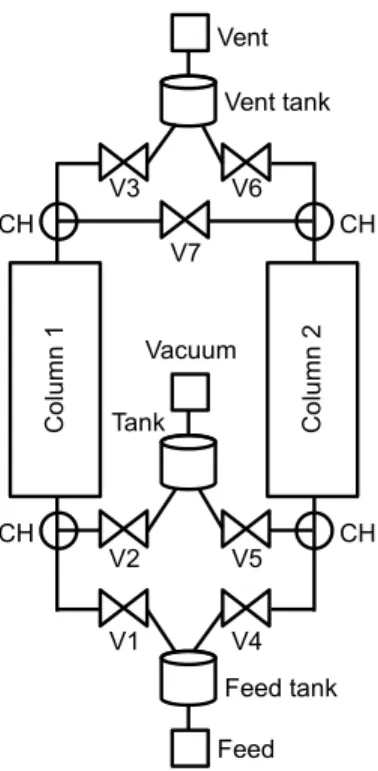
Specifically, we consider a two column, six step VPSA system as the example case study (Fig. 1). 65
This VPSA system can, depending on the adsorbent and cycle configuration, be used for a wide range of separations. For example, the system can produce the light component in an air separation process (Farooq et al., 1989) or can be used as the first stage in post-combustion carbon capture for the production of the heavy component (Park et al., 2002).
C o lu m n 2 C o lu m n 1 Feed Feed tank V1 V4 V2 V5 CH V7 V3 V6 Vent Vacuum CH CH CH Vent tank Tank
Figure 1: Schematic of the two stage extended Skarstrom cycle VPSA configuration. CH and V stand for column header and valve, respectively.
The system is symmetrical with the axis of symmetry going through the feed and vent units. On both 70
sides of each column is a column header which is typically used to ensure a homogeneous flow distribution in the column. The units labeled “Feed”, “Vacuum” and “Vent” provide the boundary conditions for the VPSA system: the Feed unit is an inlet which provides the gas mixture to separate; the Vacuum unit is an outlet which provides vacuum pressure for the purge and blowdown steps; the Vent unit is an outlet at atmospheric pressure and represents the flue gas stack in the power plant. These three units are referred to asfeed units. 75
The tanks next to the feed units buffer the flows so that the pumps can be operated continuously. The tanks and column headers are connected by valves which control the flow rates in the system and thus the cycle steps.
The operating cycle consists of the following 6 steps: pressurisation, feed, one-sided pressure equalisation, blowdown, purge and one-sided pressure equalisation. This is the original Skarstrom cycle extended by two 80
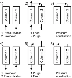
pressure equalisation steps (Skarstrom, 1966). Fig. 2 shows these 6 steps and the corresponding gas flows and connections between the two columns.
The two sides of the system are cycled through the same steps but with a half cycle offset between them. For example, during the feed step of column 1, the other column performs the purge step. The different cycle steps are defined by opening and closing the 7 valves of the system. This is illustrated by the stem 85
position of the valves: 0 indicates a closed valve, 1 an open valve and any value in between a partially open valve. The stem positions for the 6 cycle steps shown in Fig. 2 are given in Table 1. Note that due to the symmetry in the configuration,s3ands6 will be the same.
In this case study, we consider a lab-scale system with silicalite pellets (HiSiv 3000) supplied by UOP (see supplementary information for more details on the lab-scale system). The adsorption isotherm for CO2 and N2 on silicalite was taken from (Golden & Sircar, 1994). The isotherm was measured at 31.4◦C and at 68.4◦C and these data were fitted with the multi-component Langmuir isotherm
q∗i = qsbiexp −∆ ˜Hi RT P xi 1 +PNc j=1bjexp −∆ ˜Hi RT P xj . (1)
C ol um n 1 C ol um n 2 C o lu m n 1 C o lu m n 2 C ol um n 1 C ol um n 2 1 Pressurisation
2 Blowdown 1 Feed2 Purge Pressureequalisation
C ol um n 1 C ol um n 2 C o lu m n 1 C o lu m n 2 C ol um n 1 C ol um n 2 1 Blowdown 2 Pressurisation 1 Purge 2 Feed Pressure equalisation 1) 2) 3) 4) 5) 6)
Figure 2: Steps of the Skarstrom cycle with one-sided pressure equalisation.
Table 1: Stem positions for the 7 valves for the 6 cycle steps. The stem positionss3 (≡s6) ands7 are to be determined by the optimisation procedure.
Steps for column 1 Valve 1 Valve 2 Valve 3 Valve 4 Valve 5 Valve 6 Valve 7
Pressurisation 1 0 0 0 1 0 0 Feed 1 0 s3 0 1 0 s7 Pressure equalisation 0 0 0 0 0 0 1 Blowdown 0 1 0 1 0 0 0 Purge 0 1 0 1 0 s6 s7 Pressure equalisation 0 0 0 0 0 0 1
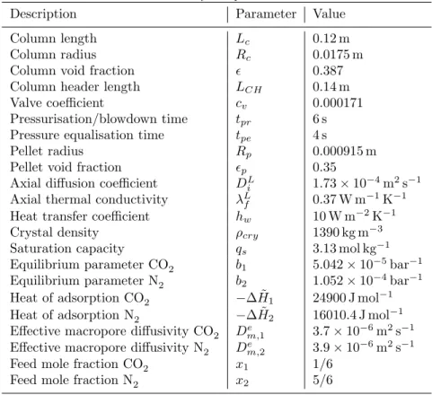
Table 2: System parameters
Description Parameter Value
Column length Lc 0.12 m
Column radius Rc 0.0175 m
Column void fraction 0.387
Column header length LCH 0.14 m
Valve coefficient cv 0.000171
Pressurisation/blowdown time tpr 6 s
Pressure equalisation time tpe 4 s
Pellet radius Rp 0.000915 m
Pellet void fraction p 0.35
Axial diffusion coefficient DL
i 1.73×10⁻⁴m2s−1
Axial thermal conductivity λL
f 0.37 W m
−1K−1
Heat transfer coefficient hw 10 W m−2K−1
Crystal density ρcry 1390 kg m−3
Saturation capacity qs 3.13 mol kg−1
Equilibrium parameter CO2 b1 5.042×10⁻⁵bar−1
Equilibrium parameter N2 b2 1.052×10⁻⁴bar−1
Heat of adsorption CO2 −∆ ˜H1 24900 J mol−1
Heat of adsorption N2 −∆ ˜H2 16010.4 J mol−1
Effective macropore diffusivity CO2 De
m,1 3.7×10⁻⁶m2s−1
Effective macropore diffusivity N2 De
m,2 3.9×10⁻⁶m2s−1
Feed mole fraction CO2 x1 1/6
Feed mole fraction N2 x2 5/6
kinetic diameter of less than 0.35 nm and silicalite has channels with width greater than 0.5 nm. We use the Linear Driving Force (LDF) model to describe the mass transfer in the macropore and assume that the adsorbed concentration in the micropore is in equilibrium with the macropore concentration. The macropore LDF parameter is calculated from the effective macropore diffusivity by
kpi = 5D e m,i Rp
.
The adsorbent parameters and the system dimensions are collected in Table 2.
To fully describe the system, the feed flow rate, feed time, vacuum pressure, feed temperature and the 90
stem positions of the purge valve (V7) and the vent valves (V3 and V6) must be specified. These will define the search space for the design optimisation problem and will be described in Section 5 below. The numerical simulator is described in the next section, and is sufficiently general to design VPSA systems with an arbitrary number and combination of units and cycle steps.
3. Dynamic adsorption cycle model 95
The VPSA system and the associated cycle shown in Fig. 1 and 2 can be simulated in two ways: i) simu-lating only the columns (Webley & He, 2000) or ii) simusimu-lating the columns and the supporting infrastructure, such as valves and tanks (Liu et al., 2011; Nikolic et al., 2008). In the former approach, the different cycle steps are defined through the boundary conditions of the columns while, in the latter approach, valves are opened and closed according to the schedule of an equivalent experimental apparatus. The former approach 100
has a slightly lower computational complexity while the latter approach is closer to the experiment. Since the increase in computational complexity is manageable and the aim is to simulate an existing experimental system, the second approach is used.
The VPSA system is build from four unit types (column, valve, tank and feed unit) and the simulations are performed with an in-house general adsorption cycle simulator. Briefly, the simulator implements the 105
mass, momentum and energy balances for adsorption columns and auxiliary units such as valves, splitters and tanks. Since the governing equations for these units have been presented previously (Banu et al., 2013; Friedrich et al., 2013), we give here only a list of the used models. However, the governing equations are repeated for completeness in the supplementary information in Appendix A.
The column model uses the axially dispersed plug flow model and the pressure drop is described by the 110
Ergun equation. The adsorption equilibrium is described by the Langmuir model and the mass transfer by the macropore LDF model. The energy balance takes heat transfers between the surroundings, column, gas phase and solid phase into account. The system of partial differential algebraic equations is discretized along the column length with a flux-limited finite volume method. The resulting system of ordinary differential algebraic equations is integrated in time with the backward differentiation formulas implemented in the 115
SUNDIALS solver (Hindmarsh et al., 2005). The system is simulated cycle after cycle until the cyclic steady state is reached.
3.1. Calculation of purity, recovery and molar work
The simulator is used to generate the composition and flow profiles to allow the calculation of the criteria considered for ranking design alternatives. The design criteria are the purity and the recovery of CO2. 120
These, together with the power requirements, are calculated, for the k-th cycle based on the number of moles passing through the relevant feed units and the work done by those units:
PuritykCO 2 = nk vac,CO2−n k−1 vac,CO2 PNc j=1 n k vac,j−n k−1 vac,j , (2) RecoverykCO 2 = nkvac,CO 2−n k−1 vac,CO2 nk f e,CO2−n k−1 f e,CO2 , (3) Molar workkCO 2 = Wk f e−W k−1 f e +W k vac−Wvack−1 nk vac,CO2−n k−1 vac,CO2 . (4)
The number of moles for any unitk,nkj,i, is a cumulative amount from the start of the process. The work done in the feed units, i.e. Wf eandWvac, is calculated from the pump power. Hence, the difference between the amounts for cyclekand cyclek−1 give the number of moles and work during thek-th cycle. The purity 125
and recovery of CO2will be the objective functions for the subsequent multi-objective optimisation and are always calculated at the ’Vacuum’ unit.
4. Surrogate based optimisation with NSGA-II
The need to simulate a dynamic system to provide the data necessary for the evaluation of the design criteria means that the optimisation of the system and cycle configuration is computationally intensive. 130
Traditionally, the computational challenge is addressed through the use of simpler models. However, these models may not capture the detail required to identify the best designs, especially in a multi-objective scenario where potentially conflicting criteria are used to evaluate and compare alternative designs. This section describes a surrogate based optimisation (SBO) procedure developed to address the computational challenge through the automatic and adaptive definition of surrogate models.
135
A surrogate model is a fast approximation of the computer model output z(x) :X →R. HereX ⊂Rd
represents the design space anddis the number of design variables. Surrogate models are typically fitted to n pre-computed input-output data points ofz(x), that is, training data (X,z) = (xj, z(xj))nj=1, and can
be used to make predictions for untried points in the design spaceX. Thus no modification of the original computer code is needed. In the multi-output setting we can assign to each output its own surrogate. 140
Kriging regression (Jin et al., 2001; S´obester et al., 2014; Stein, 1999) is a popular surrogate modelling technique for engineering design and is used in this work. Other popular techniques include polynomial response surfaces, radial basis functions (RBF), artificial neural networks (ANN), multivariate adaptive regression splines (MARS), and support vector regression (SVR) (Forrester & Keane, 2009). Kriging’s
popularity can be accredited to its ability to easily produce confidence bands for prediction, which has been 145
proven to be a highly attractive feature for exploring the design space.
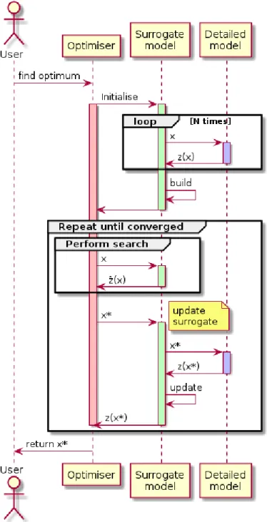
In the context of optimisation, it is possible to replace the computationally expensive objective function with a surrogate model. However, by doing so, one solves an approximation of the original optimisation problem, which may be considered a na¨ıve approach. Instead, the problem can be approached by solving a sequence of approximations of the original problem. First, employ the surrogate model in lieu of the objective 150
to assist the optimiser in the search for the next design point. Then update the surrogate model using the detailed model evaluation at some point determined by the optimisation procedure. Solve the problem again and iterate. The surrogates are updated as new input-output data points are collected from the detailed model. This procedure is illustrated in Fig. 3.
There are many potential criteria for selecting points with which to update the surrogate, referred to as 155
“surrogate based criteria.” The most common and seemingly natural choice is would be to select the design pointx with the highestz(x) value, as predicted by the surrogate. This, however, may lead to premature convergence (Jones, 2001). The expected improvement (EI) criterion (Jones et al., 1998) is another popular choice, one which guarantees convergence to a global optimum.
4.1. Kriging model 160
Kriging regression treats the computer model of interest z:X ⊆Rd →Ras an unknown deterministic
function, except for the inputs that already are known. Following (Sacks et al., 1989), we modelz(x) as a Gaussian random field,Z(x), with E Z(x)2<∞for allx∈ X. The resulting statistical model is known as the kriging model and can be used for prediction. Theordinary kriging, used in this work, is characterised by a constant mean,β ∈R, and a covariance function Σ(x,x0) =σ2K(x,x0), forx,x0 ∈ X. K(x,x0) is the
correlation function which must be positive semidefinite. A widely used correlation function is the squared exponential correlation function (Rasmussen & Williams, 2006):
K(x,x0) = exp − d X i=1 (xi−x0i) 2 2`i ! , (5)
where`= (`1, `2, . . . , `d)∈Rd+ are the correlation length-scales andσ2is the process variance.
Let us assume we have some training data D= (X,z) where X = (xj)jn=1, z = (z1, z2, . . . , zn)T, and zj = z(xj). Then, given that Z(x) is a Gaussian Process (GP), we also know that the joint distribution
¯
Z= [Z(x1), Z(x2), . . . , Z(xn)] follows a multivariate normal distribution with 1×n-dimensional mean vector 1β andn×nvariance-covariance matrixΣ(σ2,`). Here1= (1,1, . . . ,1)T and the (j, k)th element ofΣ(σ2,`)
is given by Σ(xj,xk) forxj,xk∈X. The predictive distribution ofZ(x)|`,z is a GP, with mean ˆ
z(x) = ˆβ+k(x)K−1(z−1βˆ), (6)
and variance
s2(x) = ˆσ21−kT(x)K−1k(x) +γT(x) 1TK−11−1
γ(x), (7)
where the m×1 vector k(x) has entry j given by K(x,xj) for xj ∈ X, γ(x) = 1−1TK−1k(x), and the generalized least square solution ˆβ = (1TK−11)−11TK−1z. K is the correlation matrix given by K=σ−2Σ. Here we estimate the process variance using the unbiased estimate ˆσ2= 1
n(z−1βˆ)
TK−1(z
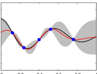
−1βˆ). Fig. 4 is an illustrative example included for readers unfamiliar with kriging modelling.
165
The kriging mean is given by (6), which is our kriging predictor, and the kriging variance is given by (7). The kriging expressions are derived under the assumption that the correlation parameters ` are known which rarely is the case. The correlation parameters`can be estimated by the data using Maximum Likelihood Estimation (MLE). The ML estimates ˆ`can be determined by minimizing the profile log-likelihood −2 lnL(`) =nlnσ2
`+ ln|K`| (Sacks et al., 1989), where L(`) is the profile likelihood under the Gaussian
170
assumption. We also add a small regularization parameterτ2>0 (known as the nugget, or the jitter) to the
diagonal elements of the correlation matrixKto improve its condition number before computing its inverse, which is required in (6) and (7). Typically,τ2 is small. This results in a kriging model (with some slightly
perturbed correlation matrix entries) that does not ensure interpolation of the given dataD. Nevertheless, the use of a regularization parameter to improve numerical stability can be advantageous (Gramacy & Lee, 175
Figure 3: Sequence diagram for a surrogate based optimiser showing when the surrogate is invoked and when the detailed model, or simulation, is invoked. This sequence is based on an optimiser that has some internal search procedure within an outer iteration; an example of such a method would be a genetic algorithm.
-1.5 -1 -0.5 0 0.5 1 1.5 0 0.2 0.4 0.6 0.8 1 x
Figure 4: Exemplary illustration of kriging, with functionz(x) (black-solid line), known input-output dataD= (X,z) (blue-solid circles), and the kriging predictor (red-dashed line) with 95%-confidence bands (grey region) produced by the kriging variance.
4.2. Kriging prediction error analysis
Over the value domains for the decision parameters considered in our case study (described in Section 5) we have assessed the prediction quality of the kriging surrogate model for both the product purity (2) and the product recovery (3). The prediction error is the normalised root-mean-square prediction error (NRMSPE):
NRMSPE = r 1 M PM j=1(ˆz(xj)−z(xj))2 maxjz(xj)−minjz(xj) , (8)
wherez(x) is the computer model output and ˆz(x) is the kriging predictor. The results of this analysis are presented in Fig. 8. To calculate the NRMSPE, a hold-off set has been used, consisting of 1,000 input-output data samples of the VPSA simulator, and determined by maximin distance Latin-hypercube sampling (LHS). 180
ML estimates are used for the parameters in the squared exponential correlation function (5). The kriging model prediction errors for both objectives are below 10% if the training data set size exceeds 60. As the number of design solutions in the training set increases beyond 60, the rate of the decrease in error slows down, as expected (Loeppky et al., 2009). The conclusion of the error analysis is that the kriging surrogates can be used for well-behaved VPSA model outputs such as purity and recovery.
185
4.3. Developing a surrogate based optimisation procedure
A standard optimisation problem is to maximise (or minimise) an objective function z(x) :X →R: x∗= arg max
x∈X
z(x). (9)
Alternatively, when the objective z(x) is expensive to evaluate, a surrogate model ˆz(x) can be used in lieu of the objective, i.e.,
ˆ
x∗= arg max
x∈X
ˆ
z(x). (10)
The solution ˆx∗ serves as an approximation to the solution of the original problem, x∗. Indeed, the more accurate the surrogate, the more confidence we will have in the solution ˆx∗. On the other hand, even with an accurate surrogate, the difference between the two solutions may be very large. In practice, therefore, the SBO method is used (Viana et al., 2014).
190
SBO exploits the predictive power of the surrogate model in lieu of the objective. First the surrogate is built on a set of training data. Then, at each iteration of the SBO method, the optimiser of choice is
0 0.05 0.1 0.15 0.2 0.25 0 20 40 60 80 100 120 140
NRMSPE to the VPSA simulator
Number of model evaluations Purity Recovery
Figure 5: NRMSPE for the kriging model based on the training data consisting of purity and recovery calculations using the detailed VPSA simulator. The error bars represent the variability over ten sets of training data (min-mean-max).
applied for a design criterion evaluated with a surrogate model. At the end of each iteration, the surrogate is updated with the design solution (xk, z(xk)) selected by the optimiser for the chosen design criterion. A common surrogate based design criterion is to just optimise the surrogate response ˆzDk(x). The procedure 195
is repeated until the stopping criteria are met.
The SBO problem for iterationk= 1,2, . . .can be written as: xk= arg max
x∈X
C(x,Dk,ˆzDk,ˆs
2
Dk;·), (11)
for some surrogate based design criterion C(·), with Dk = D0
k−1
[
i=1
(xi, z(xi)) being the input-output data known at iterationk and whereD0denotes the initial data (xi, z(xi))
n
i=1. Here ˆzDk(x) is the kriging mean (6) and ˆs2
Dk(x) is the kriging variance (7), conditioned on the training data Dk. In developing an SBO, the following must be addressed:
200
• the choice of optimiser;
• the criteria which form the objective functions; • the initial training for the surrogate;
• how to handle failures in the evaluation of the detailed model; and, • a parallel implementation, if any.
205
For the development of the SbNSGA-II SBO method, each of these is discussed in turn.
The choice of optimiser. Most conventional optimisation methods can be used within the SBO framework. We have used the Non-dominated Sorting Genetic Algorithm-II (II) (Deb et al., 2002). The NSGA-II method has been extensively used for multi-criteria design problems. It is a genetic algorithm suitable for optimisation where gradient information is not present and where any of the objective function, the 210
constraints or the design space may be non-convex. NSGA-II is able to incorporate infeasible design points into the selection procedure. It also offers diversity control for the evolving population of designs to generate an approximation to the Pareto front that is as broad as possible.
The criteria. The choice of the surrogate based criteria should ensure the surrogates adaptively target the regions of the design space believed to contain good design solutions and should guarantee convergence in the limit to the global optima. With the correct choice, the surrogate should actively learn as the search progresses. Some popular kriging-based design criteria are thekriging mean,
C(x,ˆzDk) =−zˆDk(x), (12)
thekriging variance,
C(x,sˆ2D k) = ˆs
2
Dk(x), (13)
and the expected improvement (EI) (Jones et al., 1998). The latter selects the design point xk with the largest expected improvement relative to the best known design solution:
C(x,zDk, Z(x)) =EZ(max{zmin−Z(x),0}), (14) where zmin = minzDk. Based on the Gaussian assumption for Z(x), conditioned on the known data Dk, the EI criterion can be expressed in closed-form:
C(x,zDk,zˆDk,ˆs 2 Dk) = (zmin−zˆDk(x))Φ z min−zˆDk(x) ˆ sDk(x) + ˆsDk(x)φ z min−zˆDk(x) ˆ sDk(x) (15) where Φ(·) is the cumulative distribution and φ(·) is the probability density function for the conditional posterior probability distribution of the kriging model. The EI criterion is useful when applied iteratively to 215
improve the global approximation while searching for the optima.
The kriging mean criterion tends to be too optimistic unless the objective function is easy to approximate or convex. Jones (2001) demonstrated that using an optimiser on the kriging mean can cause the method to get trapped at a local optimum and, in turn, the improvement of the surrogate stagnates. The goal of the kriging variance criterion is equivalent to learning the value at the design point of highest uncertainty and, 220
hence, strives to improve prediction accuracy rather than targeting regions of interest in the design space. SBO with the EI criterion is also known as efficient global optimization (EGO) (Jones et al., 1998). EGO has gained popularity as an SBO method but a drawback is that, if the process variance is under-estimated, the EGO search may have limited exploration as it concentrates too early on the current best solution. On the other hand, if the variance is over-estimated, the fact that the location of the currently best solution is 225
known is not exploited enough and the result is slow convergence.
Motivated by Voutchkov & Keane (2010), we use the following hybrid criterion to promote robustness:
C(x,zˆDk,sˆ 2 Dk) = (1−(−1)k) 2 zˆDk(x) + (1−(−1)k−1) 2 sˆ 2 Dk(x). (16)
This criterion is well-balanced between exploration (kriging variance) and exploitation (kriging mean), guar-antees global convergence in the limit, and is easy to interpret.
Initial training data. Prior to running the SBO algorithm, the design space is sampled to obtain the initial training data for building the kriging model. For kriging regression, a rule of thumb for the moderate size 230
of the training data is 10d (Loeppky et al., 2009). Examples of classical experimental design techniques for physical experiments are full-factorial and central composite design (Montgomery, 2007). For designing computer experiments, however, Latin hypercube sampling (McKay et al., 1979) is commonly used as it scales well to high-dimensional design spaces and is easy to implement. Our initial training data are generated through a maximin Latin hypercube design (MmLHD). First we generate a number of latin hypercube 235
design (LHD) points and the design which has the largest minimum inter-point distance is selected (maximin criterion). MmLHD could be viewed a compromise between the maximin and minimax criterion.
As another option for sampling, although not used in our work, is to sequentially design the training data. Sequential design using entropy-based criteria generally outperform LHDs (Beck & Guillas, 2014), as long as the underlying computer model is computationally expensive. We will be considering this and other 240
Handling simulation model failures. VPSA process simulations may become unstable for certain design configurations. An unstable design may cause a failure in the evaluation of the design point. In our case, simulator failures are mainly due to failure to solve the set of differential algebraic equations whenever the dynamic behaviour in the adsorbent beds is too challenging. In such a case, even if no output is returned by 245
the simulator, we still include the design point in the training data. This additional information improves the kriging variance (7). Note that the kriging variance does not explicitly depend on the output data, only implicitly via ˆσ2. The uncertainty can be modelled more accurately by accounting for the failed design
points. When the search is guided by the kriging variance, this approach helps us avoid revisiting failed design points, as well as points in close proximity.
250
Parallel implementation. The parallel implementation of the algorithm is based on the approach of Schonlau (1998) for multi-point selection, known as theKriging Believer (Janusevskis et al., 2012). In thek-th SBO iteration, n design points are selected sequentially but without evaluation until all the points have been selected. We denote thejth design point selected during thekth SBO iteration byxkj. First we selectxk1
by performing the kth SBO iteration algorithm as before. Next, we add (xk1,zˆ(xk1)) to the training data,
255
and the kriging is updated. Observe that we updated the training data with the kriging mean ˆz(xk1), instead
of the true model output z(xk1). The same steps are performed for xkj, j = 2, . . . , n, sequentially. The computer model is then evaluated in parallel for thendesign points, the training data set is corrected with {(xkj, z(xkj))}nj=1, the kriging model is updated, and the next SBO iteration begins. With this approach,
nshould be proportional to the number of allocated CPUs. The design selection becomes less efficient for 260
largen, since the training data are updated with the kriging mean at each stepj, leading to degeneracy. 4.4. The implementation of SbNSGA-II: a Surrogate based NSGA-II
This section describes the specifics of implementing an SBO based on NSGA-II for the VPSA design problem.
SBO extension to multiple objectives in NSGA-II. A kriging model is used for each objective together with a mixture of surrogate based design criteria (16), which can be written as follows:
C(x,zˆDk,ˆs 2 Dk) = (1−(−1)k) 2 zˆDk(x) + (1−(−1)k−1) 2 ˆs 2 Dk(x). (17) where ˆzDk(x) = [ˆzDk1(x), . . . ,zˆDkq(x)], ˆs 2 Dk(x) = [ˆs 2 Dk,1(x), . . . ,ˆs 2
Dk,1(x)], andq is the number of objective
265
functions. For the parallel implementation, the index kis replaced by the index j as described above. For example, should eight CPUs be available, four CPUs would be used to compute design points selected by optimising ˆzDk(x) and the other four for points selected by maximising ˆs
2 Dk(x).
What makes the NSGA-II environment more challenging with surrogates is that the optimiser is popu-lation based and returns non-dominated solutions (in a Pareto sense). First NSGA-II is applied to design 270
criterion (17). The na¨ıve approach would then be to select one (or multiple) non-dominated solutions for further consideration from the Pareto set. Instead, by respecting the nature of the multi-objective setting, the kriging-based Pareto front (from applying NSGA-II on kriging models) is combined with the current Pareto front and one or several non-dominated solutions for model evaluation are selected. This leads to a Pareto front with better diversity, richness, and coverage.
275
Transformation of purity and recovery. The kriging makes predictions on the real lineRwhereas our model
outputs, purity and recovery, are ratios in the interval [0,1]. Some predictions made by the kriging will inevitably violate physical constraints, such as concentrations. One could enforce the bounds by using the extreme values 0 and 1 whenever a prediction falls outside the feasible domain [0,1]. This manipulation of the kriging response may lead to non-differentiable behaviour. We instead suggest the following transformation of the kriging’s training dataz:
u= log
z
(1 +)1−z
, (18)
whereuis the transformed data, and >0 is a typically very small perturbation. This extends the output space from [0,1 +] to the real lineR. Then, afterwards, in order to make predictions, we transform back
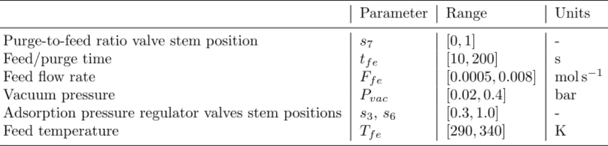
Table 3: Decision parameters
Parameter Range Units
Purge-to-feed ratio valve stem position s7 [0,1]
-Feed/purge time tf e [10,200] s
Feed flow rate Ff e [0.0005,0.008] mol s−1
Vacuum pressure Pvac [0.02,0.4] bar
Adsorption pressure regulator valves stem positions s3,s6 [0.3,1.0]
-Feed temperature Tf e [290,340] K
using ˆz(x) = ((1 +) exp(ˆu(x)))/(1 + exp(ˆu(x))), where ˆu(x) is a transformed kriging prediction. Here is a small perturbation to allow z= 1. The perturbation parameter may also be necessary to ensure the transformation is valid if any outputz(x) is above 1 due to numerical errors, e.g., producing a purity level 280
of 1.0001.
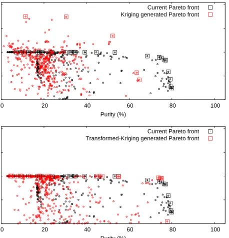
An advantage of this transformation is that, when a multi-objective optimiser is applied, the Pareto order-ing of the multi-objective function evaluations is preserved under transformation, i.e., if one response value dominates another in the original space, this response will also dominate the same one in the transformed space. Fig. 6 shows that the proposed transformation improves the algorithm’s robustness for multiple objec-285
tives with physical constraints. Other examples of transformation-based kriging models are the log-normal kriging (Diggle & Ribeiro, 2007), trans-Gaussian kriging (De Oliveira et al., 1997) using Box-Cox transfor-mations, andu= log(z+1) for non-negative outputs (Spiller et al., 2014). In fact, this data transformation is an essential ingredient to ensure the kriging-generated Pareto front scales well with the current Pareto front when combined.
290
Diversity constraint in the design space. We impose a diversity constraint in the design space to avoid clustering: if the distance between the most promising candidate design point xand the training data X, given by the Euclidean norm,
x˜− ˜ X 2= min ˜ x∗∈X˜ v u u u t d X j (˜xj−x˜∗j)2 (19)
isε−small, the candidate is rejected and the second most promising candidate is tested, and so on, until a viable candidate is found. Here ˜xand ˜X are normalised.
Stopping criteria. One of the challenges with evolutionary strategies for optimisation is to decide when to stop. In this work, we focus on the analysis of the methodology and therefore stop the algorithm when a given number of iterations have been completed. A stop criterion could also be designed with respect to some 295
computational budget or with respect to the change in the best design solution found, over a few iterations, either in terms of change in the design space or in the objective space.
5. The case study
As a case study, we use the separation of the flue gas of a coal fired power station by a VPSA process with 300
the adsorbent silicalite. The setup of the VPSA system is described in Section 2 above. In that description, a number of parameters required to fully describe the VPSA process were not defined. These form the design space and are given by the decision parameters presented in Table 3. Out of computational convenience, the decision parameters have all been normalised to [0,1] for use in the surrogate based optimisation.
While the VPSA process depends on a large number of parameters, these 6 parameters have the largest 305
impact on the process and are those usually adjusted to optimise the process performance. The purge-to-feed ratio controls the amount of gas flow during the purge step. A larger ratio usually results in faster desorption
0 50 100 150 200 0 20 40 60 80 100 Recovery (%) Purity (%)
Current Pareto front Kriging generated Pareto front
0 50 100 150 200 0 20 40 60 80 100 Recovery (%) Purity (%)
Current Pareto front Transformed-Kriging generated Pareto front
Figure 6: Top: The Pareto front approximation generated by responses from the kriging predictor. Bottom: The Pareto front approximation generated by the transformed-kriging. This illustates the benefit of using kriging in the transformed space when performing multi-objective VPSA optimisation when there are physical constraints for any of the objective functions.
but lowers the resulting purity. The feed time and flow rate influence the productivity and recovery of the process. These parameters are linked if we only consider the purity and recovery. The vacuum pressure controls how much CO2is desorbed during the purge step. The lower the vacuum pressure the more CO2is 310
desorbed but at the expense of higher energy consumption. The stem positions of the vent valves control the pressure during the feed step and thus the amount of CO2 adsorbed at equilibrium. The feed temperature influences the shape of the isotherm and thus the working capacity. At higher temperatures the isotherm becomes more linear and the desorption step might be more efficient.
While the general effect each of these parameters individually has on the performance of the VPSA 315
process is known, the interplay between these parameters and the conflicting objectives make the use of optimisation methods mandatory for the design of efficient VPSA processes.
5.1. Optimisation methods: SbNSGA-II and SbNSGA-II ALM
We use our developed SBO method presented in Section 4.3. Ordinary kriging models (see Section 4.1) are surrogate models chosen to approximate the product purity and recovery outputs and are trained on 320
transformed data, as described earlier, to ensure predictions are made in [0,1]. The kriging models assume an empirical squared exponential correlation (5) fitted using maximum likelihood estimation (MLE). A regularization parameterτ2 = 10−6 is introduced for numerical stability in the kriging computations. The empirical correlation structure is updated when new input-output data arrives. MLE is quite computationally intensive, so we only update the parameter estimates until we have 80 data points. In this case study, we 325
do not expect using more than 80 data points will lead to any significant difference in the estimate values. The initial training data is of size 16 and has been sampled as an MmLHD design.
For the NSGA-II, we have specified the following: population size Np = 128, mutation ratemr= 1/d, mutation index nm = 20, crossover rate cr = 0.9, and crossover index nc = 5, with real-coded values, simulated binary crossover (SBX) and polynomial mutation. We use ε = 10−3 for the explicit diversity 330
constraint (19) in the design space.
Two implementations have been developed, one using the NSGA-II along with the kriging mean criterion (SbNSGA-II) and one which introduces Active Learning MacKay (ALM) to construct a mixture of criteria (17) that broaden the approximation to the Pareto front (SbNSGA-II ALM). The implementations make full use of parallel computing with the Kriging believer approach and have been tested on an 8 CPU core 335
system, yielding close to linear speed up. Eight design points are selected per SBO iteration, and for those design configurations we run the VPSA model in parallel over the eight CPU cores.
5.2. Optimisation results
Two objectives are considered, the purity and the recovery, and these are maximised simultaneously in a Pareto sense. For comparison, we have also included results for the stand-alone NSGA-II, given a budget 340
of 1600 model evaluations of the VPSA simulator. We have used five separate sets of training data for SbNSGA-II to show the method’s robustness with respect to the training data.
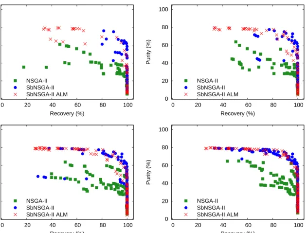
Fig. 7 shows the optimisation results of the stand-alone NSGA-II, SbNSGA-II, and SbNSGA-II ALM, at different numbers of evaluations of the VPSA simulator. Although there is only a small difference in performance between SbNSGA-II and SbNSGA-II ALM for 256 points, our criterion (17) is more robust 345
as the optimiser can escape local optima and enables active learning for the kriging model. In Fig. 7, we can see that, with some initial training data, the SbNSGA-II can be substantially worse than SbNSGA-II ALM. The benefit with SbNSGA-II is its fast convergence when close to the optima. The Pareto front for the SBO methods using 256 design points overlaps with the Pareto front for the stand-alone NSGA-II using a normally excessive budget of 1600 design points (see bottom left in Fig. 8). The SBO methods reach a 350
reliable Pareto solution. A trade-off between the SBO methods can be achieved by modifying the mixture criterion of the SbNSGA-II ALM to use the predictive mean criterion more frequently than the predictive variance criterion.
The ML estimates of the parameters in the squared exponential correlation function (5) are `purity = (1.2,4.7,1.6,15,14.4,15)T, and `
recovery = (3.2,1.8,1.7,5.6,8.5,15)T. The parameter order in the vectors
355
is the same order as introduced in Table 3. These correlation parameters represent the importance of the different parameters on the respective outputs and can be used to guide the analysis of the optimised design. A small value of a correlation parameter indicates a strong nonlinear relationship between the objective and the design parameter. Thus, parameters with lower values have a large influence on the objective. On the
0 20 40 60 80 100 0 20 40 60 80 100 Purity (%) Recovery (%) NSGA-II SbNSGA-II SbNSGA-II ALM 0 20 40 60 80 100 0 20 40 60 80 100 Purity (%) Recovery (%) NSGA-II SbNSGA-II SbNSGA-II ALM 0 20 40 60 80 100 0 20 40 60 80 100 Purity (%) Recovery (%) NSGA-II SbNSGA-II SbNSGA-II ALM 0 20 40 60 80 100 0 20 40 60 80 100 Purity (%) Recovery (%) NSGA-II SbNSGA-II SbNSGA-II ALM
Figure 7: Results using different optimisation strategies. Top left: 64 evaluations of the high-fidelity simulation, right: 96. Bottom left: 176, right: 256. The results for the different strategies are produced by combining five Pareto fronts resulting from using five different initial training data.
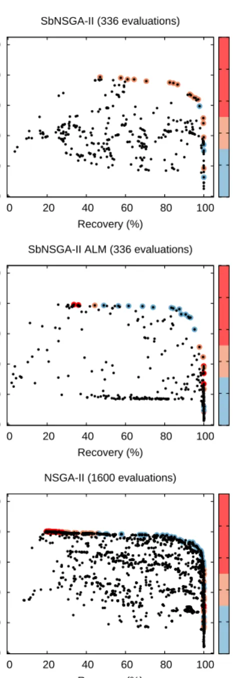
0 20 40 60 80 100 0 20 40 60 80 100 Purity (%) Recovery (%) SbNSGA-II (336 evaluations) 0 20 40 60 80 100
Power consumption per mole (kJ/mol)
0 20 40 60 80 100 0 20 40 60 80 100 Purity (%) Recovery (%) SbNSGA-II ALM (336 evaluations)
0 20 40 60 80 100
Power consumption per mole (kJ/mol)
0 20 40 60 80 100 0 20 40 60 80 100 Purity (%) Recovery (%) NSGA-II (1600 evaluations) 0 20 40 60 80 100
Power consumption per mole (kJ/mol)
other hand, for a large value of a correlation parameter, the objective function is smooth with respect to 360
the corresponding design parameter. While this indicates that the relationship has no significant nonlinear behaviour, it does not indicate that the design parameter has no influence at all on the objective. The possible linear relationship can be deduced from the high level visualization given in Fig. 9.
While the optimisation performed above only considered the purity and recovery, the power consumption is essential for the design of an effective VPSA system. For the design solutions, we also calculated the 365
system’s power consumption defined by (4). Fig. 8 shows on the Pareto fronts the power consumption per mole highlighted by the color range. The power consumption for our SbNSGA-II ALM and NSGA-II agree along the whole Pareto front and both show a minimum at the bend of the Pareto front. This is to be expected because at the bend the system recovers most of the CO2 at a high purity. Interestingly, the SbNSGA-II optimisation does not show a clear minimum at the bend of the Pareto front. The reason for 370
this higher power consumption of the solutions is not obvious but is probably due to the limited exploration of the design space of SbNSGA-II.
5.3. Discussion
The low values of the correlation parameters`purity and`recoverytell us that the purge-to-feed ratio has a large influence on the purity and that the feed/purge time and the feed flowrate have a large influence on 375
the recovery. The purge flow controlled by the purge-to-feed ratio consists mostly of the light component and thus the purity of the heavy component is reduced by a large value of this ratio. If the product of the feed/purge time and the feed flowrate are too large, a part of the heavy component will break through during the feed step which will reduce the recovery. Thus these relationships are expected and it is more interesting to investigate why the other parameters have a lower influence.
380
To investigate the influence of the design parameters with higher values of the correlation parameters, we need to also consider the high level visualisation presented in Fig. 9. The link between the different Pareto front segments highlighted with colours (cyan, red, green, and blue) and the design solutions is revealed in Fig. 9. This link enables us to better understand the underlying process. For example, in the regime of high purity, we can see that the purge valve should be closed during the feed/purge step. This is reasonable as 385
the CO2is the heavy product taken out during the feed step and to purge the second bed with a gas mixture of highN2 is likely to deteriorate the CO2 level of the outgoing product.
The two correlation parameters for the feed temperature are at the upper limits and thus it seems that the feed temperature has little influence on the outputs. Since the CO2 isotherm on silicalite is nonlinear at the lower temperature and becomes more linear towards the upper boundary of the feed temperature, 390
we would have assumed that the feed temperature has at least some influence on the purity and recovery. However, the high level visualisation in Fig. 9 shows that the feed temperature varies without any discernible trend, confirming that the feed temperature has very little influence on either the purity or recovery. This very low influence can be explained by the large column headers in the CCSi VPSA unit (see Table 2). The column headers act like heat exchangers so that, even for the highest feed temperature, the gas entering 395
the adsorption column is cooled to almost room temperature. Thus the feed temperature has almost no influence on the processes in the adsorption column and this validates the use of the estimated correlation parameters in combination with Fig. 9 as a sensitivity analysis tool.
According to the correlation parameters, the vacuum and adsorption pressure have some influence on the recovery. The two pressure values influence the working capacity of the system. For a larger pressure 400
range, i.e. the difference between vacuum and adsorption pressure, the working capacity of the adsorbent is larger and thus the amount of CO2adsorbed in each cycle increases. This increases the recovery because the losses of CO2 in each cycle to the vent are not increasing accordingly. On the other hand, the correlation parameter for the purity is at the upper limit, indicating, similar to the feed temperature, that the pressures have little influence on the purity. While Fig. 9 confirms that there is no trend in the feed pressure, this 405
is not true for the vacuum pressure which is at the lower limit except for the design points with very low purity, i.e. at or close to the feed concentration. It is intuitively clear that a sufficiently low vacuum pressure is required to efficiently remove the adsorbed CO2 from the bed. Thus the best performance in terms of CO2 purity is achieved when the vacuum pressure is at its lowest point in the specified range. This shows that for high values of the correlation parameters it is essential to also look at the high level visualisation. 410
0 20 40 60 80 100 0 20 40 60 80 100 Purity (%) Recovery (%) Segment 1 Segment 2 Segment 3 Segment 4 0 0.2 0.4 0.6 0.8 1
s7 tfe Ffe Pvac s3,s6 Tfe Purity Recovery
Variable values (normalised)
Variables and objectives Parallel Coordinates 0 20 40 60 80 100 0 20 40 60 80 100 Purity (%) Recovery (%) Segment 1 Segment 2 Segment 3 Segment 4 0 0.2 0.4 0.6 0.8 1
s7 tfe Ffe Pvac s3,s6 Tfe Purity Recovery
Variable values (normalised)
Variables and objectives Parallel Coordinates
Figure 9: Pareto front divided into segments (Left) by colours. Parallel coordinates visualisation (Right) shows that the design solutions associated with different Pareto front segments are clustered. The top figures are for the NSGA-II (1600 evaluations), and the bottom ones are for the SbNSGA-II ALM (320 evaluations). The SbNSGA-II ALM, with only 320 evaluations, provides a sufficient approximation of the Pareto curve as well as the associated design solutions.
The product of feed/purge time and feed flowrate is crucial to achieve high purity and high recovery. If the product is large, the adsorption front will break through at the vent end of the column. This will lead to high purity CO2streams in the purge step but will yield a low recovery. If the product is small, none of the CO2 will leave the column at the vent end and thus the system will have a high recovery but a low purity. 415
To reach a system with a high purity and high recovery the product of feed/purge time and feed flowrate needs to be an intermediate value which ensures that the adsorption front almost reaches the vent end of the adsorption column. As we move the adsorption front closer to the vent side of the column, a small amount of CO2 is breaking through at the vent side. By increasing the purge-to-feed ratio, a larger percentage of this CO2is recovered which explains the influence of the purge-to-feed ratio on the recovery.
420
It is interesting to note that the power consumption per mole of CO2 shown in Fig. 8 increases from the bend for decreasing purity but goes back to the minimum value for very low purities. These low purities are similar to the feed mole fraction and could be achieved without any separation at the vent side of the system. However, the purity and recovery are always calculated at the vacuum side. The high level visualisation shows that, for these cases, both the feed/purge time and feed flowrate are at very low values. This indicates 425
that the flow through the system is low and that only a small amount of the feed gas leaves the system at the vent side.
While the power consumption and productivity are not as important for a demonstration system, these are critical in large scale applications. For example, the low vacuum pressure of 0.02 bar, while achievable in a small lab-scale or demonstration unit, would be difficult to reach in large scale industrial applications and 430
would lead to large power consumption. Furthermore, a high productivity of the process is crucial for small and light systems. This is important for small scale portable units, e.g. portable oxygen concentrators, as well as for large scale industrial units, e.g. carbon capture units for fossil fuel power station.
This discussion shows that the correlation parameters together with the high level visualisation in Fig. 9 are a valuable tool in the analysis of the optimisation results. The high level visualisation, in particular, helps 435
to understand the interplay between different decision variables and the trade-off between purity and recovery. Multi-objective visualization methods can be a valuable tool to explore the relationship between competing objectives for the promising VPSA designs (˘Zilinskas et al., 2015). For example, the lines connecting the feed/purge time and feed flowrate for each segment of the Pareto front, i.e. lines of the same colour, are almost all crossing. This indicates that the amount of feed gas (tf e×Ff e) for each segment of the Pareto 440
front is almost constant. This shows that the feed/purge time and feed flowrate are linked with respect to purity and recovery, i.e. purity and recovery depend only on the amount of feed gas. However, the two design parameters are independent with respect to power consumption and productivity and this will be investigated in a future publication.
6. Conclusion 445
In this work, we propose the first multi-objective optimisation method that involves the use of kriging surrogate models for providing fast solutions to the design of VPSA systems. We have demonstrated its efficiency against the standard NSGA-II and verified its robustness by analysing the performance using five different initial training data. It is well-known that surrogate based optimisation involving multiple objectives is challenging. We propose a transformation of the objective space during the training phase of 450
the surrogate models (for the purity and recovery) to constrain their response space to [0,1] (i.e., to obey the physical constraints). This modification leads to better predictions of the Pareto front.
We have developed two implementations, SbNSGA-II and SbNSGA-II ALM, which both outperform the standard NSGA-II. II ALM has been shown to be more robust than II, although SbNSGA-II displays a stronger convergence when close to the optima. Both SBO methods achieved a reduction in the 455
number of VPSA model simulations by a factor between 2 and 5, depending on the desired resolution of the Pareto curve approximation. This reduction in the number of high-fidelity simulations directly translates to a reduction in the computational time and thus enables the efficient optimisation of VPSA systems. Furthermore, the power consumption of the solutions of SbNSGA-II ALM is comparable with the solutions of NSGA-II, while the solutions of SbNSGA-II show a significantly higher power consumption in the high 460
purity and high recovery region. While the inclusion of power consumption and productivity as objectives is beyond the scope of this contribution, the multi-objective SBO framework is capable of handling more than two objectives and this will be investigated in the future.
A further advantage of the SBO methods is the calculation of the correlation parameters. Together with the high level visualisation these parameters offer significant information about the interplay between the 465
decision variables and objectives. This insight can be used to analyse the optimisation results and to guide further optimisation studies.
Appendix A. Supplementary information
Appendix A.1. Carbon Capture and Storage Interactive Unit
The Carbon Capture and Storage interactive (CCSi) unit was built by the University of Edinburgh in 470
collaboration with SciFun (http://www.scifun.ed.ac.uk). The rigs primary function is to demonstrate the idea of carbon capture using vacuum/pressure swing adsorption (VPSA) at science and engineering fairs. Once it is not used for this purpose anymore, it will be refitted and recalibrated for scientific experiments. The rig is shown in Fig. A.10.
Figure A.10: Picture of the CCSi unit
The rig is split into three sections: generation, capture and storage. Of these the generation and storage 475
sections are only representations of the actual process while the capture unit is a fully functioning VPSA unit. The generation section represents a typical power plant in which electricity is generated by the burning of fossil fuels. The resulting flue gas is routed to the capture section. Since the combustion is only simulated, compressed air and carbon dioxide cylinders are used to generate a simulated flue gas of 1/6 CO2 with the remainder air.
480
As shown in the diagram the rig uses LED lights which show the valve configurations. In Fig. A.10, the valves are set to divert the flue gas to the capture unit which separates CO2from the flue gas. The capture unit makes use of a six step, two column VSA process. The flue gas enters at a feed flowrate of 3 L/min and a pressure of 1.3 bar. The raffinate leaves the top of the column at atmospheric pressure through the power station chimney stack. The chimney stack has a sensor with inbuilt LED indicators which measures 485
the concentration of CO2 leaving in the raffinate stream. The extract (CO2rich) stream leaves the process under a vacuum of 0.1 bar. The columns are 0.3 m long and have an inner diameter of 0.035 m. The two
columns are filled with approximately 0.08 kg of silicalite pellets (HiSiv 3000) supplied by UoP. This amount of silicalite fills about 0.12 m of each column. The remainder (evenly split between the top and bottom of the columns) is filled with solid beads.
490
Once the CO2 has been separated, the gas flows to the storage section. The storage section shown in Fig. A.10 illustrates the use of a geological structure for the storage of CO2.
Appendix A.2. Governing equations
The following paragraphs present the governing mass, energy and momentum balance equations for the column, CSTR, valve and feed unit.
495
Column. The flow through the packed bed is described by the axial dispersed plug flow model. More detailed models, e.g. including radial dispersion, are generally not necessary (Ruthven, 1984) while the ideal plug flow can be approximated by letting the dispersion coefficient go to zero. For the plug flow model the mass and energy balance in the column are given by the following equations.
∂ci ∂t =− 1− dQ¯i dt − ∂(v·ci) ∂z − ∂Ji ∂z, (A.1) dQ¯i dt =p dcm i dt + (1−p) dq¯i dt =k p i Ap Vp (ci−cmi ), (A.2) dq¯i dt =k cr i 3 Rcr (qi∗−q¯i), (A.3) ∂ ˇ Uf ∂t =−(1−) ∂Uˇp ∂t − ∂ Hˇf ·v ∂z − ∂JT ∂z − Nc X i=1 ∂JiH˜i ∂z −hw Ac Vc (Tf−Tw), (A.4) ∂Uˇp ∂t =p ∂Uˇp,f ∂t + (1−p) ∂Uˇp,s ∂t =hp Ap Vp (Tf−Tp), (A.5) ρwˆcP,w ∂Tw ∂t =−hw Ac Vw (Tw−Tf)−U Aco Vw (Tw−T∞). (A.6)
Due to the large heat capacity of the wall the wall temperature calculated by Eq. A.6 is almost constant; thus in this contribution the wall is assumed to be isothermal, i.e. Eq. A.6 is not used.
The mass and heat transfer into the pellet depend on the mass and heat transfer coefficient and the ratio of the pellet surface area to pellet volume. In this contribution the pellets were assumed to be spherical so that Ap/Vp = 3/Rp. The mass transfer into the adsorbent crystals assumes that the crystals are spherical with radius Rcr. The pellet void fraction, p, is the ratio of the macropore volume over the total pellet volume. The macropore LDF parameter is calculated from the effective macropore diffusivity
Dm,ie = p τ 1 Dm i + 1 DK i −1 (A.7) where the individual diffusion coefficient are given by
Dmi = 1.60×10⁻⁷ q T3 M W−1 1 +M W −1 2 P σ2 12Ω12 DKi = 97rpore r T M Wi
HereM Wiis the molecular weight in g mol−1,σ12is the collision diameter from the Lennard-Jones potential
in A, Ω12is a function depending on the Lennard-Jones force constant and temperature andrporethe mean pore radius in m.
The thermal diffusive flux JT and the diffusive flux of componentiin the fluid phaseJi are given by JT =−λLf ∂Tf ∂z −λ L p(1−) ∂Tp ∂z , Ji=−DLicT ∂xi ∂z. (A.8)
Here the axial thermal conductivity in the fluid and pellet are given by λL
f and λ
L
p, respectively, and the axial dispersion coefficient byDiL.
The boundary conditions for the gas phase concentrations and the enthalpy are given by the Danckwerts boundary conditions for flow into the column and the no diffusive flux for flow out of the column. With the conventions that the positive flow directions is from 0 toLc these can be written in a combined form as
JT|z=0= v+|v| 2 ˇ Hf,0−−Hˇf,0 (A.9) JT|z=Lc= v− |v| 2 ˇ Hf,L+ c − ˇ Hf,Lc (A.10) Ji|z=0= v+|v| 2 ci,0−−ci,0 (A.11) Ji|z=Lc= v− |v| 2 ci,L+ c −ci,Lc (A.12) where the superscripts − and + indicate the concentration values to the left and right of the boundary, respectively.
The constitutive equations for the energy terms are given by ˇ Uf =cTU˜f,ref+cT Z Tf Tref ˜ cVdT, ˇ Hf =cTH˜f,ref +cT Z Tf Tref ˜ cPdT, ˇ Up=pUˇp,f+ (1−p) ˇUp,s ˇ Up,f =cmTU˜p,f,ref+cmT Z Tp Tref ˜ cmVdT, ˇ Up,s= ˇUsol+ ˇUads, ˇ
Usol=ρcryUˆsol,ref +ρcry
Z Tp
Tref
ˆ
cP,soldT,
ˇ
Uads= ˇHads =qTH˜ads,ref+qT
Z Tp Tref ˜ cP,adsdT− −∆ ˇHads Tp, −∆ ˇHads Tp= Nc X i=1 Z qi 0 −∆ ˜Hi Tp,qj6=i dq, ˜ Hi= ˜Hi,ref + Z Tf Tref ˜ cP,idT. ˇ
Usol and ˇUads are the internal energy per unit volume in the adsorbent and the adsorbed phase, respectively. 505
Here the tilde indicates the molar quantities and the subscript “ref” indicates the reference value atTref and Pref. The total concentration in the fluid phase and in the macropore are given bycT andcmT, respectively. ρcry is the crystal density, qT is the total adsorbed concentration in the micropore and ˆcP,sol is the specific heat capacity at constant pressure in the solid phase. The total heat of adsorption per unit volume ∆ ˇHads is calculated from the component heat of adsorptions ∆ ˜Hi.
510
˜
cP and in the adsorbed phase ˜cP,ads are calculated from the respective component heat capacities by
˜ cV = Nc X i=1 xi˜cV,i, ˜cP = Nc X i=1 xi˜cP,i, ˜ cP,ads= Nc X i=1 qi qT ˜ cP,i, c˜mV = Nc X i=1 xmi ˜cV,i.
The superscript m indicates the macropore concentrations and heat capacities and xi are the component mole fractions.
The pressure drop along the column is given by the Ergun equation −dP dz = 150µ(1−)2 2(2R p)2 v+1.75(1−)ρf 2Rp v|v|. (A.13)
Continuously stirred tank. The column header and the tanks are modelled as continuously stirred tanks with an arbitrary number of connectionsNI. The governing equations are given by
Fj=−Fnj, j= 1, . . . , NI, (A.14) Vdci dt = NI X j=1 F j+|Fj| 2 ci,nj cT ,nj +Fj− |Fj| 2 ci cT , (A.15) dUf dt = NI X j=1 F j+|Fj| 2 ˜ Hf,nj+ Fj− |Fj| 2 ˜ Hf +hwA(Tw−Tf). (A.16)
The pressure in the tank is calculated from the temperature and total gas concentration by the ideal gas law. Equation A.14 requires that the flow rate is provided by the neighbouring units. For the inlets connected to either a valve or feed unit, this is fulfilled since these units calculate the flow rate from the composition and temperature. However, for the inlet connected to the column, the flow rate needs to be provided. Here the flow rate is calculated by
F =k(Pn−P). (A.17)
With a sufficiently large value of the coefficientk, the pressure drop between the column header and column will be neglible.
Valve. The flow rate through the valve is calculated by
F =sjcvcT s
|P0−P1|
ρf
(A.18)
where cv is the valve coefficient,P0 and P1 are the pressures at the two inlets, respectively,cT is the total 515
concentration and ρf is the fluid density. The stem position,sj, of the valve indicates if the valve is open or closed. Here 0 indicates a closed valve, 0.5 a half open valve and 1 a fully open valve. The simulator allows the opening and closing of valves at specified times. Through the coordinated operation of the valves, different steps in the cycle, e.g. blowdown and pressure equalisation, are performed (see Table 1). Pressure, temperature and gas composition are passed through the valve to the neighbouring units.
520
Feed unit. Pressure, temperature and feed composition are kept constant at the initial conditions. The flow rate is set according to
F = Fi, P−PPn >0.01, Fi,0.5 1 + cos 100π 0.01− P−PPn , otherwise. (A.19)
Here, Fi is the set flow rate andP and Pn are the pressures in the feed unit and the neighbouring unit, respectively.
The feed unit also calculates the number of moles of each component to pass through the outlet and the power consumption of the blower or vacuum pump. The number of moles is calculated through the following ODEs dni dt = F+|F| 2 ci,n cT ,n +F− |F| 2 ci cT , (A.20)
with initial values of ni= 0. Since the sign on the right hand side of equation A.20 changes with the flow direction, this equation gives a positive result if more molecules have entered the feed unit than have left the feed unit and a negative results otherwise.
525
The power consumption is calculated by
P ow= γ γ−1RT F Pn Patm γ−1γ −1 , ifPn > Patmand F <0, γn γn−1RTnF Patm Pn γnγn−1 −1 , ifPn < Patmand F >0, 0, otherwise. (A.21) dW dt =P ow, W(0) = 0 (A.22) Hereγ= ˜cP ˜
cV is the ratio of the molar heat capacities at constant pressure and constant volume. Table A.4: Nomenclature
Parameter Description Units
A Surface area m2
Ac Inner surface area of the column m2
Aco Outer surface area of the column m2
Ap Pellet surface area m2
bi Equilibrium parameter of comp.i bar−1
ci Concentration of componenti mol m−3
ˆ
cP Specific heat capacity J kg−1K−1
˜
cP Molar heat capacity at constant pressure J mol−1K−1
cT Total concentration mol m−3
cv Valve coefficient m2
√ 10−5
˜
cV Molar heat capacity at constant volume J mol−1K−1
DiK Knudsen diffusion coefficient of comp.i m2s−1
Dim Molecular diffusion coefficient of comp.i m2s−1
Dm,ie Effective macropore diffusivity of comp.i m2s−1
DL
i Effective axial dispersion coefficient of comp.i m2s−1
F Molar flow rate mol s−1
Ff e Feed flow rate mol s−1
hp Pellet-to-fluid heat transfer coefficient W m−2K−1
hw Fluid-to-wall heat transfer coefficient W m−2K−1
−∆ ˜Hi Heat of adsorption of comp.i J mol−1
ˇ
H Enthalpy per unit volume J m−3
˜
H Molar enthalpy J mol−1
Ji Diffusive flux of comp. iin the fluid phase mol m−2s−1
JT Thermal diffusive flux in the fluid phase J m−2s−1
k Flow rate coefficient mol s−1bar−1
kcr
i LDF coefficient of comp.iin the adsorbent crystal m s−1
kpi LDF coefficient of comp.iin the pellet m s−1
Lc Column length m
ni Number of moles of comp.i mol
nk
Table A.4: Nomenclature
Parameter Description Units
P Pressure bar
Pvac Vacuum pressure bar
¯
qi Sorbate concentration of comp.i mol m−3
qs Saturation capacity mol m−3
q?
i Sorbate concentration of comp.iat equilibrium mol m−3
qT Total adsorbed concentration mol m−3
¯
Qi Concentration of comp.i in the pellet mol m−3
R Gas constant J mol−1K−1
Rc Column radius m
Rcr Crystal radius m
Rp Pellet radius m
sj Stem position of valvej
-tf e Feed/purge time s
T Temperature K
Tf e Feed temperature K
U Internal energy J
ˇ
U Internal energy per unit volume J m−3
v Interstitial velocity m s−1
V Volume m3
Vc Column volume m3
Vp Pellet volume m3
Vw Column wall volume m3
W Work J
xi Mole fraction of comp.i
γ Ratio of heat capacities at constant pressure and volume
δw Column wall thickness m
Column void fraction
p Pellet void fraction
-λL Effective axial thermal dispersion coefficient W m−1K−1
µ Fluid viscosity Pa s
ρ Density kg m−3
τ Pore tortuosity of the pellet
-Subscript
ads Adsorbed phase
atm Atmospheric
c Column
f Fluid phase
n Neighbouring unit
p Pellet
ref Reference state
s Solid phase
sol Adsorbent phase
w Column wall ∞ Surroundings Superscript cr Crystal L Axial m Macropore p Pellet