LQR and H_2 Controllers Design Using State Derivative Feedback for Multivariable Systems

(1)

http://asrjetsjournal.org/

LQR and

𝐇𝐇

𝟐𝟐

Controllers Design Using State Derivative

Feedback for Multivariable Systems

Hazem I. Ali

a

*, Mohammed Z. M. Ali

b

a,b_{Department of control and system engineering, University of Technology, Baghdad-10001, Iraq} a_{Email: [email protected]}

b_Email:_{[email protected]}

Abstract

This paper presents the design of LQR (linear quadratic regular) and H₂ controller using state derivative

feedback. This design is solvable for all controllable systems. The state derivative feedback is used instead of state feedback in many mechanical systems because the main sensors of vibration are accelerometers. A multivariable active suspension system is used in this paper to show the effectiveness of the proposed controllers. The obtained results are compared to the same approaches when a state feedback is used. It is shown that the design using state derivative feedback can achieve a better performance.

Keywords: LQR control; H₂ control; state derivative feedback; multivariable systems; active suspension. 1. Introduction

The state derivative feedback is very useful and essential for achieving a desired specification for some control problems. The motivation of using state derivative feedback comes from controlled vibration suspension of mechanical systems where the accelerometers represent the main sensors of vibration [1]. Different approaches that are based on state feedback have been extended to be designed using state derivative feedback. Linear quadratic regulator (LQR) is considered one of the well-known approaches that provide practical feedback gains. This method has adopted either feedback or derivative feedback controller and it provides a perfect stabilization for an active suspension system [2]. The LQR approach can achieve an acceptable performance of the system by minimizing the performance index [3]. Based on LQR, some of new control algorithms have been derived such as in [1,4].

--- * Corresponding author.

(2)

The H₂ is used to find the optimal gain matrices the achieve the desired performance. The H₂ optimal control is used in the design of state feedback control by minimizing a quadratic performance index of the system and attenuating the effect of disturbances. Reference [5] have used the state derivative feedback for direct algorithm for the pole placement for multi input linear system. Reference [6] used state derivative feedback for

Pole-placement for single input single output systems. Cardimand his colleagues [7] used state derivative feedback

for linear control systems. Kataria and his colleagues [8] used state derivative feedback for Pole-placement

problem. Wangand his colleagues [9] have used the state feedback H₂ control with regional pole assignment.

Reference [10] presented a technique based on state derivative for robust vibration control of dynamical systems.

In this paper, the design of LQR and H₂ controllers are presented using state derivative feedback. The proposed controllers are applied to a multivariable active suspension.

2. Controllers Design

In this section, the solutions of LQR optimal control and H₂ robust control using state derivative feedback are presented.

2.1. LQR State Derivative Feedback Problem Formulation

Consider a continuous, time-invariant, linear system:

𝑥𝑥̇(𝑡𝑡)= 𝐴𝐴𝑥𝑥(𝑡𝑡) +𝐵𝐵𝐵𝐵(𝑡𝑡) (1)

The objective is to stabilize the system by means of a linear state derivative feedback expressed by:

𝐵𝐵(𝑡𝑡) =−𝐾𝐾𝑥𝑥̇(𝑡𝑡) (2)

The control law in equation (2) is to stabilize the system with a desired performance. The closed-loop system dynamics is:

𝑥𝑥̇(𝑡𝑡)=𝐴𝐴_𝑐𝑐𝑥𝑥(𝑡𝑡) (3)

where

𝐴𝐴𝑐𝑐=(𝐼𝐼+𝐵𝐵𝐾𝐾)−1𝐴𝐴 (4)

The stabilizing control with good dynamic behavior is achieved by minimizing a quadratic cost or performance index of the type [1]:

𝐽𝐽(𝑥𝑥̇(𝑡𝑡),𝐵𝐵(𝑡𝑡)=∫₀∞(𝑥𝑥̇(𝑡𝑡)𝑄𝑄𝑥𝑥(𝑡𝑡) +𝐵𝐵𝑇𝑇(𝑡𝑡)𝑅𝑅𝐵𝐵(𝑡𝑡))𝑑𝑑𝑡𝑡 (5)

(3)

𝐽𝐽 =∫₀∞(𝑥𝑥̇𝑄𝑄𝑥𝑥+ (𝐾𝐾𝑥𝑥̇)𝑇𝑇𝑅𝑅(𝐾𝐾𝑥𝑥̇))𝑑𝑑𝑡𝑡=∫ 𝑥𝑥̇₀∞ 𝑇𝑇(𝑄𝑄+𝐾𝐾𝑇𝑇𝑅𝑅𝐾𝐾)𝑥𝑥̇𝑑𝑑𝑡𝑡 (6)

Suppose that a constant positive semidefinite symmetric matrix 𝑃𝑃that satisfy equation (6) can be obtained, thus 𝑥𝑥̇𝑇𝑇₍_𝑄𝑄₊_𝐾𝐾𝑇𝑇_{𝑅𝑅𝐾𝐾}₎_𝑥𝑥̇₌₋𝑑𝑑

𝑑𝑑𝑑𝑑(𝑥𝑥𝑇𝑇𝑃𝑃𝑥𝑥) =−𝑥𝑥̇𝑇𝑇𝑃𝑃𝑥𝑥 − 𝑥𝑥𝑇𝑇𝑃𝑃𝑥𝑥̇ (7) then, equation (7) can be rewritten as:

𝑥𝑥̇𝑇𝑇₍_𝑄𝑄₊_𝐾𝐾𝑇𝑇_{𝑅𝑅𝐾𝐾}₎_𝑥𝑥̇₌_{−𝑥𝑥̇}𝑇𝑇₍_{𝑃𝑃𝐴𝐴} 𝑐𝑐 −1₊_𝐴𝐴 𝑐𝑐 −𝑇𝑇_𝑃𝑃₎_𝑥𝑥̇₍₈₎ where 𝐴𝐴𝑐𝑐−1=𝐴𝐴−1(𝐼𝐼+𝐵𝐵𝐾𝐾) =𝐴𝐴−1+𝐴𝐴−1𝐵𝐵𝐾𝐾 (9)

Comparing both sides of equation (8),

𝑃𝑃𝐴𝐴𝑐𝑐−1+𝐴𝐴𝑐𝑐−𝑇𝑇𝑃𝑃+𝐾𝐾𝑇𝑇𝑅𝑅𝐾𝐾+𝑄𝑄= 0 (10)

where

𝐴𝐴𝑐𝑐−𝑇𝑇=𝐾𝐾𝑇𝑇𝐵𝐵𝑇𝑇𝐴𝐴−𝑇𝑇+𝐴𝐴−𝑇𝑇 (11)

Substituting equation (9) and (11) in equation (10),

𝑃𝑃(𝐴𝐴−1₊_𝐴𝐴−1_{𝐵𝐵𝐾𝐾}_{) + (}_𝐾𝐾𝑇𝑇_𝐵𝐵𝑇𝑇_𝐴𝐴−𝑇𝑇₊_𝐴𝐴−𝑇𝑇₎_𝑃𝑃₊_𝐾𝐾𝑇𝑇_{𝑅𝑅𝐾𝐾}₊_𝑄𝑄_{= 0}₍₁₂₎

then, equation (12) can be rewritten as:

𝑃𝑃𝐴𝐴−1₊_{𝑃𝑃𝐴𝐴}−1_{𝐵𝐵𝐾𝐾}₊_𝐾𝐾𝑇𝑇_𝐵𝐵𝑇𝑇_𝐴𝐴−𝑇𝑇_𝑃𝑃₊_𝐴𝐴−𝑇𝑇_𝑃𝑃₊_𝐾𝐾𝑇𝑇_{𝑅𝑅𝐾𝐾}₊_𝑄𝑄_{= 0}₍₁₃₎

Since 𝑅𝑅is positive-definite symmetric matrix, then

𝑅𝑅=𝑇𝑇𝑇𝑇_𝑇𝑇₍₁₄₎

where 𝑇𝑇is a nonsingular matrix. Substituting equation (14) in equation (13), yields:

𝑃𝑃𝐴𝐴−1₊_𝐴𝐴−𝑇𝑇_𝑃𝑃₊₍_{𝑇𝑇𝐾𝐾}₊_𝑇𝑇−𝑇𝑇_𝐵𝐵𝑇𝑇_𝐴𝐴−𝑇𝑇_𝑃𝑃₎𝑇𝑇₍_{𝑇𝑇𝐾𝐾}₊_𝑇𝑇−𝑇𝑇_𝐵𝐵𝑇𝑇_𝐴𝐴−𝑇𝑇_𝑃𝑃₎_{− 𝑃𝑃𝐴𝐴}−1_{𝐵𝐵𝑇𝑇}−1_𝑇𝑇−𝑇𝑇_𝐵𝐵𝑇𝑇_𝐴𝐴−𝑇𝑇_𝑃𝑃₊_𝑄𝑄_{= 0}₍₁₅₎_The minimization of 𝐽𝐽 requires the minimization of the following:

𝑥𝑥̇𝑇𝑇₍_{𝑇𝑇𝐾𝐾}₊_𝑇𝑇−𝑇𝑇_𝐵𝐵𝑇𝑇_𝐴𝐴−𝑇𝑇_𝑃𝑃₎𝑇𝑇₍_{𝑇𝑇𝐾𝐾}₊_𝑇𝑇−𝑇𝑇_𝐵𝐵𝑇𝑇_𝐴𝐴−𝑇𝑇_𝑃𝑃₎_𝑥𝑥̇₍₁₆₎

(4)

𝑇𝑇𝐾𝐾=−𝑇𝑇−𝑇𝑇_𝐵𝐵𝑇𝑇_𝐴𝐴−𝑇𝑇_𝑃𝑃₍₁₇₎

The optimal gain matrix 𝐾𝐾 is:

𝐾𝐾 =−𝑅𝑅−1_𝐵𝐵𝑇𝑇_𝐴𝐴−𝑇𝑇_𝑃𝑃₍₁₈₎

Finally, the optimal stabilizing control law is given by:

𝐵𝐵(𝑡𝑡) =𝑅𝑅−1_𝐵𝐵𝑇𝑇_𝐴𝐴−𝑇𝑇_{𝑃𝑃𝑥𝑥̇}₍_𝑡𝑡₎₍₁₉₎

The matrix 𝑃𝑃 in equation (19) must satisfy equation (13) or the following algebraic Riccati equation (ARE):

𝑃𝑃𝐴𝐴−1₊_𝐴𝐴−𝑇𝑇_{𝑃𝑃 − 𝑃𝑃𝐴𝐴}−1_{𝐵𝐵𝑅𝑅}−1_𝐵𝐵𝑇𝑇_𝐴𝐴−𝑇𝑇_𝑃𝑃₊_𝑄𝑄_{= 0}₍₂₀₎

2.2. 𝑯𝑯𝟐𝟐 State Derivative Feedback Problem Formulation

Consider a linear time invariant system expressed by:

𝑥𝑥̇(𝑡𝑡) =𝐴𝐴𝑥𝑥(𝑡𝑡) +𝐵𝐵1𝑑𝑑(𝑡𝑡) +𝐵𝐵2𝐵𝐵(𝑡𝑡) (21)

𝑒𝑒(𝑡𝑡) =𝐶𝐶1𝑥𝑥̇(𝑡𝑡) +𝐷𝐷12𝐵𝐵(𝑡𝑡) (22)

𝑍𝑍(𝑡𝑡) =𝑥𝑥̇(𝑡𝑡) (23)

The following assumptions are made:

1. The system matrix 𝐴𝐴 is of full rank. 2. (𝐴𝐴, 𝐵𝐵₁) and (𝐴𝐴, 𝐵𝐵₂) are stabilizable. 3. (𝐶𝐶₁, 𝐴𝐴) is detectable.

4. All state derivative measurements are possible.

The objective of this work is to obtain a scalar state derivative feedback control law described by:

𝐵𝐵(𝑡𝑡) =−𝐾𝐾𝑥𝑥̇(𝑡𝑡) (24)

Assuming that 𝑑𝑑(𝑡𝑡) is the white noise vector with unit intensity, then [11]:

‖𝑇𝑇𝑒𝑒𝑑𝑑‖𝐻𝐻22=𝐸𝐸(𝑒𝑒𝑇𝑇(𝑡𝑡)𝑒𝑒(𝑡𝑡)) (25)

(5)

𝑒𝑒𝑇𝑇_𝑒𝑒₌_𝑥𝑥̇𝑇𝑇_𝐶𝐶

1𝑇𝑇𝐶𝐶1𝑥𝑥̇+ 2𝑥𝑥̇𝑇𝑇𝐶𝐶1𝑇𝑇𝐷𝐷12𝐵𝐵+𝐵𝐵𝑇𝑇𝐷𝐷12𝑇𝑇𝐷𝐷12𝐵𝐵 (26) The minimization of ‖𝑇𝑇_{𝑒𝑒𝑑𝑑}‖_𝐻𝐻2₂ is equivalent to the solution of the stochastic regulator problem by setting: 𝑄𝑄=𝐶𝐶1𝑇𝑇𝐶𝐶1 , 𝑁𝑁=𝐶𝐶1𝑇𝑇𝐷𝐷12 , 𝑅𝑅=𝐷𝐷12𝑇𝑇𝐷𝐷12 then 𝐸𝐸�𝑒𝑒𝑇𝑇₍_𝑡𝑡₎_𝑒𝑒₍_𝑡𝑡₎_�₌_{𝐽𝐽�𝑥𝑥̇}₍_𝑡𝑡_),_𝐵𝐵₍_𝑡𝑡₎_�₌_∫∞₍ 0 𝑥𝑥̇𝑇𝑇(𝑡𝑡)𝑄𝑄𝑥𝑥(t) + 2𝑥𝑥̇𝑇𝑇(t)𝑁𝑁𝐵𝐵(t) +𝐵𝐵𝑇𝑇(t)𝑅𝑅𝐵𝐵(t))𝑑𝑑𝑡𝑡 (27) and 𝐽𝐽�𝑥𝑥̇(𝑡𝑡),𝑣𝑣(𝑡𝑡)�=∫₀∞(𝑥𝑥̇𝑇𝑇₍_𝑡𝑡₎_𝑄𝑄 𝑚𝑚𝑥𝑥̇(t) +𝑣𝑣𝑇𝑇(t)𝑅𝑅𝑣𝑣(t))𝑑𝑑𝑡𝑡 (28) where 𝑄𝑄𝑚𝑚=𝑄𝑄 − 𝑁𝑁𝑅𝑅−1𝑁𝑁𝑇𝑇 (29) 𝑣𝑣(t) =𝐵𝐵(t) +𝑅𝑅−1_𝑁𝑁𝑇𝑇_𝑥𝑥̇₍_𝑡𝑡₎₍₃₀₎

Consequently, the system in equation (21) will be rewritten as:

𝑥𝑥̇(𝑡𝑡) =𝐴𝐴𝑚𝑚𝑥𝑥(𝑡𝑡) +𝐵𝐵1𝑑𝑑(𝑡𝑡) +𝐵𝐵2𝑣𝑣(𝑡𝑡) (31)

where

𝐴𝐴𝑚𝑚=𝐴𝐴 − 𝐵𝐵2𝑅𝑅−1𝑁𝑁𝑇𝑇 (32)

In term of 𝑣𝑣(𝑡𝑡) and from equation (30), the optimal state derivative feedback is:

𝑣𝑣(𝑡𝑡) =−𝐾𝐾𝑚𝑚𝑥𝑥̇(𝑡𝑡) (33)

where

𝐾𝐾𝑚𝑚=𝐾𝐾 − 𝑅𝑅−1𝑁𝑁𝑇𝑇 (34)

Substitute equation (33) in equation (31), the system equation will be:

𝑥𝑥̇(𝑡𝑡) =𝐴𝐴𝑚𝑚𝑥𝑥(𝑡𝑡) +𝐵𝐵1𝑑𝑑(𝑡𝑡)− 𝐵𝐵2K𝑚𝑚𝑥𝑥̇(𝑡𝑡) =𝐴𝐴𝑛𝑛𝑥𝑥(𝑡𝑡) +𝐵𝐵1𝑑𝑑(𝑡𝑡) (35)

where

(6)

Substitute equation (33) in equation (28), the objective function will be:

𝐽𝐽�x(𝑡𝑡),𝑣𝑣(𝑡𝑡)�=∫₀∞(𝑥𝑥̇𝑇𝑇₍_𝑡𝑡₎₍_𝑄𝑄

𝑚𝑚+𝐾𝐾𝑚𝑚𝑇𝑇𝑅𝑅𝐾𝐾𝑚𝑚)𝑥𝑥(t))𝑑𝑑𝑡𝑡 (37) Suppose that, it can be found a constant positive simidefinite symmetric 𝑃𝑃 that satisfy equation (37),

𝑥𝑥̇𝑇𝑇₍_𝑡𝑡₎₍_𝑄𝑄

𝑚𝑚+𝐾𝐾𝑚𝑚𝑇𝑇𝑅𝑅K𝑚𝑚)𝑥𝑥̇(t) =−_{𝑑𝑑𝑑𝑑}𝑑𝑑�𝑥𝑥𝑇𝑇(𝑡𝑡)𝑃𝑃𝑥𝑥(𝑡𝑡)�=−𝑥𝑥̇𝑇𝑇(𝑡𝑡)𝑃𝑃𝑥𝑥(𝑡𝑡)− 𝑥𝑥𝑇𝑇(𝑡𝑡)𝑃𝑃𝑥𝑥̇(𝑡𝑡) (38) Therefore, the performance index can be obtained as:

𝐽𝐽�𝑥𝑥̇(𝑡𝑡),𝑣𝑣(𝑡𝑡)�=∫₀∞(𝑥𝑥̇𝑇𝑇₍_𝑡𝑡₎_𝑄𝑄

𝑚𝑚𝑥𝑥̇(t) + (𝐾𝐾𝑚𝑚𝑥𝑥̇(t))𝑇𝑇𝑅𝑅(𝐾𝐾𝑚𝑚𝑥𝑥̇(t)))𝑑𝑑𝑡𝑡=−𝑥𝑥𝑇𝑇(𝑡𝑡)𝑃𝑃𝑥𝑥(𝑡𝑡)|0∞=−𝑥𝑥𝑇𝑇(∞)𝑃𝑃𝑃𝑃(∞) +

𝑥𝑥𝑇𝑇₍₀₎_{𝑃𝑃𝑥𝑥}₍₀₎₍₃₉₎

Assume that the closed loop system is asymptotically stable, then 𝑥𝑥(∞) →0. Therefore the performance index can be obtained in terms of initial conditions and matrix 𝑃𝑃 as:

𝐽𝐽=𝑥𝑥𝑇𝑇₍₀₎_{𝑃𝑃𝑥𝑥}₍₀₎₍₄₀₎

From equation (35), the following relationship can be obtained:

𝑥𝑥(𝑡𝑡) =𝐴𝐴𝑛𝑛−1𝑥𝑥̇(𝑡𝑡) +𝐵𝐵1𝑑𝑑(𝑡𝑡) (41)

where

𝐴𝐴𝑛𝑛−1=𝐴𝐴𝑚𝑚−1(𝐼𝐼+𝐵𝐵2𝐾𝐾𝑚𝑚) (42)

Then equation (38) can be rewritten as:

𝑥𝑥̇𝑇𝑇₍_𝑡𝑡₎₍_𝑄𝑄

𝑚𝑚+𝐾𝐾𝑚𝑚𝑇𝑇𝑅𝑅𝐾𝐾𝑚𝑚)𝑥𝑥̇(t) =−𝑥𝑥̇𝑇𝑇(𝑡𝑡)(𝑃𝑃𝐴𝐴𝑛𝑛−1+𝐴𝐴𝑛𝑛−𝑇𝑇𝑃𝑃)𝑥𝑥̇(t) (43) By comparing the two sides of equation (43), we obtain:

𝑃𝑃𝐴𝐴−1𝑛𝑛 +𝐴𝐴𝑛𝑛−1𝑃𝑃+𝐾𝐾𝑚𝑚𝑇𝑇𝑅𝑅𝐾𝐾𝑚𝑚+𝑄𝑄𝑚𝑚= 0 (44)

Substituting equation (42) in equation (44), one can obtain:

𝑃𝑃(𝐴𝐴𝑚𝑚−1(𝐼𝐼+𝐵𝐵2𝐾𝐾𝑚𝑚)) + (𝐴𝐴𝑚𝑚−1(𝐼𝐼+𝐵𝐵2𝐾𝐾𝑚𝑚))𝑇𝑇𝑃𝑃+𝐾𝐾𝑚𝑚𝑇𝑇𝑅𝑅𝐾𝐾𝑚𝑚+𝑄𝑄𝑚𝑚= 0 (45)

then, equation (45) can be rewritten as:

𝑃𝑃𝐴𝐴𝑚𝑚−1+𝐴𝐴𝑚𝑚−𝑇𝑇𝑃𝑃+𝑃𝑃𝐴𝐴𝑚𝑚−𝑇𝑇𝐵𝐵2𝐾𝐾𝑚𝑚+𝐾𝐾𝑚𝑚𝑇𝑇𝐵𝐵2𝑇𝑇𝐴𝐴−𝑇𝑇𝑚𝑚𝑃𝑃+𝐾𝐾𝑚𝑚𝑇𝑇𝑅𝑅𝐾𝐾𝑚𝑚+𝑄𝑄𝑚𝑚= 0 (46)

(7)

be rewritten as:

𝑃𝑃𝐴𝐴−1𝑚𝑚 +𝐴𝐴𝑚𝑚−𝑇𝑇𝑃𝑃+𝑃𝑃𝐴𝐴−1𝑚𝑚𝐵𝐵2𝐾𝐾𝑚𝑚+𝐾𝐾𝑚𝑚𝑇𝑇𝐵𝐵2𝑇𝑇𝐴𝐴𝑚𝑚−𝑇𝑇𝑃𝑃+𝐾𝐾𝑚𝑚𝑇𝑇𝑇𝑇𝑇𝑇𝑇𝑇𝐾𝐾𝑚𝑚+𝑄𝑄𝑚𝑚= 0 (47)

By reformulating equation (47), the following equation can be obtained:

𝑃𝑃𝐴𝐴𝑚𝑚−1+𝐴𝐴𝑚𝑚−𝑇𝑇𝑃𝑃 (𝑇𝑇𝐾𝐾𝑚𝑚+𝑇𝑇−𝑇𝑇𝐵𝐵2𝑇𝑇𝐴𝐴𝑚𝑚−𝑇𝑇𝑃𝑃)𝑇𝑇(𝑇𝑇𝐾𝐾𝑚𝑚+𝑇𝑇−𝑇𝑇𝐵𝐵2𝑇𝑇𝐴𝐴𝑚𝑚−𝑇𝑇𝑃𝑃)− 𝑃𝑃𝐴𝐴𝑚𝑚−1𝐵𝐵2𝑅𝑅−1𝐵𝐵2𝑇𝑇𝐴𝐴𝑚𝑚−𝑇𝑇𝑃𝑃+𝑄𝑄𝑚𝑚= 0 (48)

The minimization of 𝐽𝐽 requires the minimization of

𝑥𝑥̇𝑇𝑇₍_{𝑇𝑇𝐾𝐾}₊_𝑇𝑇−𝑇𝑇_𝐵𝐵𝑇𝑇_𝐴𝐴−𝑇𝑇_𝑃𝑃₎𝑇𝑇₍_{𝑇𝑇𝐾𝐾}₊_𝑇𝑇−𝑇𝑇_𝐵𝐵𝑇𝑇_𝐴𝐴−𝑇𝑇_𝑃𝑃₎_𝑥𝑥̇₍₄₉₎

Since the last expression is nonnegative, the minimum occurs when it is zero

𝑇𝑇𝐾𝐾𝑚𝑚+𝑇𝑇−𝑇𝑇𝐵𝐵2𝑇𝑇𝐴𝐴𝑚𝑚−𝑇𝑇𝑃𝑃= 0 (50)

The optimal gain matrix 𝐾𝐾_𝑚𝑚 is:

𝐾𝐾𝑚𝑚=−𝑇𝑇−1𝑇𝑇−𝑇𝑇𝐵𝐵2𝑇𝑇𝐴𝐴𝑚𝑚−𝑇𝑇𝑃𝑃=−𝑅𝑅−1𝐵𝐵2𝑇𝑇𝐴𝐴𝑚𝑚−𝑇𝑇𝑃𝑃 (51)

Finally, the optimal stabilizing control is:

𝑣𝑣(𝑡𝑡) =−𝐾𝐾𝑚𝑚𝑥𝑥̇(𝑡𝑡) =𝑅𝑅−1𝐵𝐵2𝑇𝑇𝐴𝐴𝑚𝑚−𝑇𝑇𝑃𝑃𝑥𝑥̇(𝑡𝑡) (52)

Substituting equation (52) in equation (30) yields:

𝐵𝐵(𝑡𝑡) =𝑅𝑅−1_𝐵𝐵

2𝑇𝑇𝐴𝐴𝑚𝑚−𝑇𝑇𝑃𝑃𝑥𝑥̇(𝑡𝑡)− 𝑅𝑅−1𝑁𝑁𝑇𝑇𝑥𝑥̇(𝑡𝑡) (53) then

𝐾𝐾 =−𝑅𝑅−1_[_𝐵𝐵

2𝑇𝑇(𝐴𝐴 − 𝐵𝐵2𝑅𝑅−1𝑁𝑁𝑇𝑇)−𝑇𝑇𝑃𝑃 − 𝑁𝑁𝑇𝑇] (54) The equations of the closed loop system using state derivative feedback H₂ control are:

𝑥𝑥̇(𝑡𝑡) =𝐴𝐴𝑐𝑐𝑥𝑥(𝑡𝑡) +𝐵𝐵1𝑑𝑑(𝑡𝑡) +𝐵𝐵𝑐𝑐𝑟𝑟(𝑡𝑡) (55)

𝑦𝑦(𝑡𝑡) =𝐶𝐶𝑥𝑥(𝑡𝑡) (56)

where

𝐴𝐴𝑐𝑐 = (𝐼𝐼+𝐵𝐵2𝐾𝐾)−1(𝐴𝐴 − 𝐵𝐵2𝐶𝐶) (57)

(8)

3. Illustrative Example

A multivariable active suspension system, shown in Figure 1 is used to show the effectiveness of the proposed controllers. The system dynamics can be represented by a state space model as [7]:

⎣ ⎢ ⎢ ⎡𝑥𝑥̇1(𝑡𝑡) 𝑥𝑥̇2(𝑡𝑡) 𝑥𝑥̇3(𝑡𝑡) 𝑥𝑥̇4(𝑡𝑡)⎦ ⎥ ⎥ ⎤ =













−

s s s s c c c c

m

b

m

b

m

k

m

k

M

b

M

b

M

k

M

k

2 2 2 2 2 2 1 2 2 1

1

0

1

0

⎣ ⎢ ⎢ ⎡𝑥𝑥_𝑥𝑥1(𝑡𝑡) 2(𝑡𝑡) 𝑥𝑥3(𝑡𝑡) 𝑥𝑥4(𝑡𝑡)⎦ ⎥ ⎥ ⎤ +













−

s c c

m

M

1

0

1

0

𝐵𝐵(𝑡𝑡) (59) �𝑦𝑦_𝑦𝑦1(𝑡𝑡) 2(𝑡𝑡)�=













0

1

0

1

⎣ ⎢ ⎢ ⎡𝑥𝑥_𝑥𝑥1(𝑡𝑡) 2(𝑡𝑡) 𝑥𝑥3(𝑡𝑡) 𝑥𝑥4(𝑡𝑡)⎦ ⎥ ⎥ ⎤ (60)

where 𝑀𝑀_𝑐𝑐 represents a car mass, 𝑚𝑚_𝑠𝑠 represents the driver plus seat mass. The stiffness 𝑘𝑘₁ and the damping 𝑏𝑏₁ represent the shock absorbers by which the vertical vibration caused by a street may be partially attenuated. The stiffness 𝑘𝑘₂ and the damping b2 represent the car seat suspension elements by which the undesirable vibrations subjected to the driver can be reduced. The control inputs 𝐵𝐵₁(𝑡𝑡) and 𝐵𝐵₂(𝑡𝑡).can be changed to increase the damping of vibration of the masses 𝑀𝑀_𝑐𝑐 and 𝑚𝑚_𝑠𝑠.

The accelerations signals 𝑥𝑥̈₁(𝑡𝑡) and 𝑥𝑥̈₂(𝑡𝑡) are only available for feedback because they are measured by accelerometers sensors. Depending on their measured time derivatives, the velocities 𝑥𝑥̇₁(𝑡𝑡) and 𝑥𝑥̇₂(𝑡𝑡) can be estimated. Now, the accelerations and velocities signals are available and the proposed method can be used to solve the problem.

(9)

The nominal system parameters are taken as follows [7]: 𝑏𝑏₁(damping) = 4 × 103 Ns/m,𝑏𝑏₂(damper of the seat suspension) = 5 × 102 Ns/m, 𝑘𝑘₁ (stiffness)= 4 × 104 N/m,𝑘𝑘₂ (stiffness)= 5 × 103 N/m, 𝑀𝑀_𝐶𝐶 (mass of the car)= 1500kg, 𝑚𝑚_𝑠𝑠(mass of the driver) = 70kg.

3.1. LQR Controller Results

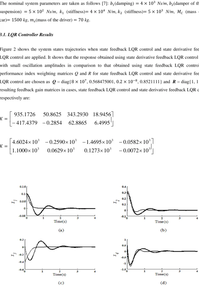
Figure 2 shows the system states trajectories when state feedback LQR control and state derivative feedback LQR control are applied. It shows that the response obtained using state derivative feedback LQR control is fast with small oscillation amplitudes in comparison to that obtained using state feedback LQR control. The

performance index weighting matrices Q and R for state feedback LQR control and state derivative feedback

LQR control are chosen as Q = diag{8 × 107, 0.568475001, 0.2 × 10−8, 0.8521111} and R = diag{1, 1}. The resulting feedback gain matrices in cases, state feedback LQR control and state derivative feedback LQR control respectively are: 𝐾𝐾=













−

417

.

4379

0

.

2854

62

.

8865

6

.

4995

9456

.

18

2930

.

343

8625

.

50

1726

.

935

𝐾𝐾=













×

−

×

−

×

−

×

−

×

3 3 3 3 3 3 3 3

10

0072

.

0

10

1273

.

0

10

0629

.

0

10

1000

.

1

10

0582

.

0

10

4695

.

1

10

2590

.

0

10

6024

.

4

Figure 2: System trajectories using state feedback LQR control (dotted line) and state derivative feedback LQR control (solid line).

(10)

3.2. 𝑯𝑯𝟐𝟐 Controller Results

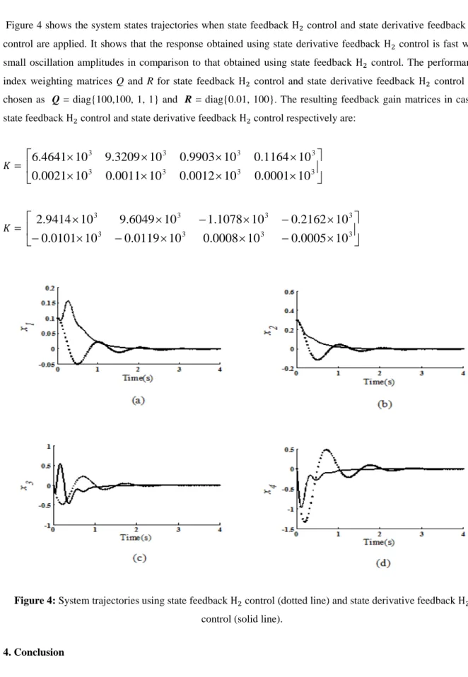
Figure 4 shows the system states trajectories when state feedback H₂ control and state derivative feedback H₂ control are applied. It shows that the response obtained using state derivative feedback H₂ control is fast with small oscillation amplitudes in comparison to that obtained using state feedback H₂ control. The performance index weighting matrices Q and R for state feedback H₂ control and state derivative feedback H₂ control are

chosen as Q = diag{100,100, 1, 1} and R = diag{0.01, 100}. The resulting feedback gain matrices in cases,

state feedback H₂ control and state derivative feedback H₂ control respectively are:

𝐾𝐾=













×

3 3 3 3 3 3 3 3

10

0001

.

0

10

0012

.

0

10

0011

.

0

10

0021

.

0

10

1164

.

0

10

9903

.

0

10

3209

.

9

10

4641

.

6

𝐾𝐾=













×

−

×

−

×

−

×

−

×

−

×

3 3 3 3 3 3 3 3

10

0005

.

0

10

0008

.

0

10

0119

.

0

10

0101

.

0

10

2162

.

0

10

1078

.

1

10

6049

.

9

10

9414

.

2

Figure 4: System trajectories using state feedback H₂ control (dotted line) and state derivative feedback H₂ control (solid line).

4. Conclusion

In this paper the LQR and H₂ controllers have been designed using state derivative feedback. The H₂ optimal control has been derived using state derivative feedback similar to LQR to find the optimal gain matrices that

(11)

achieve the desired performance. The two designed approaches were applied to a multivariable active suspension system. It was found that the designed LQR and H₂ controllers using state derivative feedback can given a better performance in comparison to the same approaches using state feedback.

References

[1]. T. H. S. Abdelaziz and M. Valask, “State Derivative Feedback By LQR For Linear Time-Invariant

System”, Proceedings of the 16th IFAC World Congress, Czech Republic, 2005, pp. 933-938.

[2]. M. Pourebrahim and A. S. Ghafari, “Designing a LQR Controller for an

Electro-Hydraulic-Actuated-Clutch Model”, International conference on Control Science and Systems Engineering, 2016.

[3]. H. I. Ali, “Mixed LQR/H-Infinity Controller Design For Uncertain Multivariable Systems”, Emirates

Journal for Engineering Research, 2015, Vol. 20, No. 1, PP. 79-85.

[4]. Rodrigues C. R. and Kuiava R. and Ramos R.A., “Design of a linear quadratic regulator for nonlinear

systems modeled via norm bounded linear differential inclusions”, Proceedings of the 18th World Congress, Milano(Italy), 2011.

[5]. T. H. S. Abdelaziz and M.Valask, “Direct Algorithm For Pole Placement By State-Derivative

Feedback For Multi-Input Linear Systems - Nonsingular Case”, Kybernetika, 2005, Vol. 41, No. 5, pp. 637-660.

[6]. T. H. S. Abdelaziz and M.Valask, “Pole-placement for SISO linear systems by state-derivative

feedback”, Acta Polytechnica, 2003, Vol. 43, No. 6, pp. 52-60.

[7]. R. Cardim, M. C. M. Teixeira, E. Assuncao and F. A. Faria, “Control Designs for Linear Systems

Using State-Derivative Feedback”, Systems Structure and Control, Pert Husek, 2008.

[8]. J. Kataria, M. K. Madhav and A. Kumar, “State Derivative Feedback Control Application for Pole

Placement Problem”, International Journal of Emerging Technology, 2014, Vol. 4, No. 4, pp. 79-85.

[9]. G. S. Wang, B. Liang and G. R. Duan, “H2-Optimal Control with Regional Pole Assignment via State

Feedback, International Journal of Control”, Automation, and Systems, 2006, Vol. 4, No. 5, pp. 653-659.

[10]. E. Reithmeier and G. Leitmann, “Robust Vibration Control of Dynamical Systems based on Derivative

of the State”, Archive Appl. Mechanics,, 2003, Vol. 72, PP. 856-864.

http://asrjetsjournal.org/