Universidade de São Paulo
2014-10
Label construction for multi-label feature
selection
Brazilian Conference on Intelligent Systems, 3th, 2014, São Carlos.
http://www.producao.usp.br/handle/BDPI/48632
Downloaded from: Biblioteca Digital da Produção Intelectual - BDPI, Universidade de São Paulo
Biblioteca Digital da Produção Intelectual - BDPI
Label Construction for Multi-label Feature Selection
Newton Spolaˆor, Maria Carolina Monard
Laboratory of Computational Intelligence Institute of Mathematics and Computer Science
University of S˜ao Paulo S˜ao Carlos, Brazil
Grigorios Tsoumakas
Machine Learning and Knowledge Discovery Group Department of Informatics
Aristotle University of Thessaloniki Thessaloniki, Greece
{newtonspolaor,hueidianalee}@gmail.com, [email protected],[email protected]
Huei Diana Lee
Laboratory of Bioinformatics Western Paran´a State University
Foz do Iguac¸u, Brazil
Abstract—Multi-label learning handles datasets where each instance is associated with multiple labels, which are of-ten correlated. As other machine learning tasks, multi-label learning also suffers from the curse of dimensionality, which can be mitigated by dimensionality reduction tasks, such as feature selection. The standard approach for multi-label feature selection transforms the multi-label dataset into single-label datasets before using traditional feature selection algorithms. However, this approach often ignores label dependence. This work proposes an alternative method,LCFS, which constructs new labels based on relations between the original labels to augment the label set of the original dataset. Afterwards, the augmented dataset is submitted to the standard multi-label feature selection approach. Experiments using Information Gain as a measure to evaluate features were carried out in 10 multi-label benchmark datasets. For each dataset, the quality of the features selected was assessed by the quality of the classifiers built using the features selected by the standard approach in the original dataset, as well as in the dataset constructed by fourLCFSsettings. The results show that setting LCFS with simple strategies using pairs of labels gives rise to better classifiers than the ones built using the standard approach in the original dataset. Moreover, these good results are accomplished when a small number of features are selected. Keywords-feature ranking; filter feature selection; Binary Relevance; Information Gain; systematic review
I. INTRODUCTION
In multi-label learning, each instance is associated with multiple labels simultaneously. A key difference between multi-label and traditional binary or multi-class single-label learning is that the labels in multi-label learning are not mutually exclusive. Thus, in comparison with traditional single-label learning, multi-label learning is more general and more challenging to solve.
that describes the dataset, as well as, or even better than the original set of features does [1], is an effective way to mitigate the curse of dimensionality.
The standard approach for multi-label Feature Selection (FS), which transforms the multi-label dataset into single-label datasets before using traditional FS algorithms, is im-plementable within the Binary Relevance (BR) approach [2]. A drawback ofBRis that label dependence is often ignored. An alternative to reduce this problem would be to construct labels based on relations among the original labels and include the new labels during the feature selection phase. The main idea of variable (label or feature) construction is to gather information about the relations among the original variables from data and infer additional variables. Although feature construction methods are less usual than feature selection methods [3], they have already been used for single-label and multi-label learning [4]. Nevertheless, to the best of our knowledge, there is little research on label construction for multi-label data.
In this work, we propose the Label Construction for Feature Selection (LCFS) method to build binary variables (new labels) based on label relationships. These variables are then included as new labels in the original dataset and the standard multi-label FS approach is used in the augmented dataset to select features. Afterwards, the dataset described by the selected features and the original labels can be submitted to any multi-label learning algorithm. Experiments in 10 benchmark datasets using the Information Gain (IG) measure for FS, suggest that settingLCFS with simple strategies in pairs of labels gives rise to better classifiers than the ones built using the standard approach when a small number of features are selected.
2014 Brazilian Conference on Intelligent Systems 2014 Brazilian Conference on Intelligent Systems
II. BACKGROUND
This section presents basic concepts and terminology of multi-label learning and feature selection.
A. Multi-label learning
Let D be a dataset composed of N examples Ei xi, Yi,i 1. . . N. Each example (instance)Ei is associ-ated with a feature vectorxi xi1, xi2, . . . , xiMdescribed by M features (attributes) Xj,j 1. . . M, and its multi-labelYi, which consists of a subset of labelsYibL, where L y1, y2, . . . , yqis the set ofqlabels. TableIshows this representation. In this scenario, the multi-label classification task consists in generating a classifier H which, given an unseen instance E x,?, is capable of accurately predicting its multi-labelY,i.e.,HE Y.
Table I MULTI-LABEL DATA
X1 X2 . . . XM Y E1 x11 x12 . . . x1M Y1
E2 x21 x22 . . . x2M Y2
EN xN1 xN2 . . . xN M YN
1) Categorizing multi-label learning algorithms:
Multi-label learning methods can be organized into two main categories [2]: (i) problem transformation methods, where the multi-label learning problem is decomposed into a set of single-label (binary or multi-class) learning tasks; and (ii) algorithm adaptation methods, which adapt specific learning algorithms to handle multi-label datasets directly. The key philosophy of the problem transformation methods is to fit data to algorithms, while for the algorithm adaptation methods is to fit algorithms to data [5].
Another categorization, proposed by Zhang and Zhou [5], organizes multi-label learning methods based on the order of label dependence taken into account, as exploring label dependence during learning can improve its performance. First-order strategies ignore co-existence of other labels. The problem transformation Binary Relevance (BR) approach ex-emplifies this category by transforming a multi-label dataset intoqlabel binary datasets, learning from each single-label problem separately and combining the results. Second-order strategies consider pairwise relations between labels, such as interactions between any pair of labels, or the ranking between relevant and irrelevant labels. High-order strategies consider relations among more labels.
Although high-order strategies potentially model wider label dependences, they are usually computationally more demanding. This work focuses on finding second-order re-lations between single labels from the multi-label dataset and representing them as new labels. The idea is that, by labeling instances with the original and the constructed labels, it will
be possible to allow feature selection methods based onBR
to incorporate label pairwise information.
2) Evaluation Measures: Unlike single-label
classifica-tion where the classificaclassifica-tion of a new instance has only two possible outcomes, correct or incorrect, multi-label classification should also take into account partiallycorrect classification. A complete discussion on multi-label evalua-tion measures, which can optimize different aspects, is out of the scope of this work and can be found in [2]. In what follows, we describe the four measures used in this work.
F-measure, Hamming Loss and Accuracy, defined by
Equations 1 to 3, are example-based evaluation measures, whereΔrepresents the symmetric difference of two sets,Yi andZiare the true and the predicted multi-label respectively.
F-measureH, D 1 SDS Q SDS i 1 2SYi9ZiS SZiS SYiS . (1) Hamming lossH, D 1 SDS Q SDS i 1 SYiΔZiS SLS . (2) AccuracyH, D 1 SDS Q SDS i 1 SYi9ZiS SYi8ZiS . (3)
In addition,Micro-averaged F-measure(Fb), defined by Equation 4, is a label-based measure, where TPyi, FPyi, TNyi and FNyi represent, respectively, the number of true/false positives/negatives for a labelyj>L.
FbH, D 2Pq j 1TPyj 2Pq j 1 TPyj q P j 1 FPyj q P j 1 FNyj . (4)
All these performance measures range in the interval
0,1. ForHamming Loss, the smaller the value, the better the multi-label classifier performance is, while for the other measures, greater values indicate better performance.
B. Feature selection
Regardless of the multi-label learning approach, any FS method addresses a few relevant issues, such as the interac-tion with the learning algorithm and the feature importance measure. Three approaches determine different types of interaction: wrapper, embedded and filter [1]. In particular, the first two approaches involve strong interaction. On the other hand, filters use general properties of the dataset to remove unimportant features from it, regardless of the learning algorithm. Thus, although the features chosen may not be the best ones for a specific learning algorithm, filter FS is performed only once for all learning algorithms. The FS algorithms used in this work fall within this approach.
Many measures have been used to estimate the importance of features based on properties of the dataset. A popular single-label FS measure is Information Gain (IG), which evaluates each feature according to the dependence between this feature and a single label, as defined by Equation5.
248
IG D, Xj entropy D v
Dv entropy Dv
D . (5)
In other words, the IG of feature Xj, j 1. . . M, calculates the difference between the entropy of the dataset D and the weighted sum of the entropy of each subset Dv D, where Dv consists in the set of examples where Xj has the valuev. Therefore, ifXjhas10distinct values1 inD, the sum would be applied to10differentDvdatasets.
III. RELATED WORK ON MULTI-LABELFS Feature selection has been an active research topic in supervised learning, with many related publications and comprehensive surveys [1]. Although most publications are related to single-label learning, a number of papers have recently reported results to support multi-label learning.
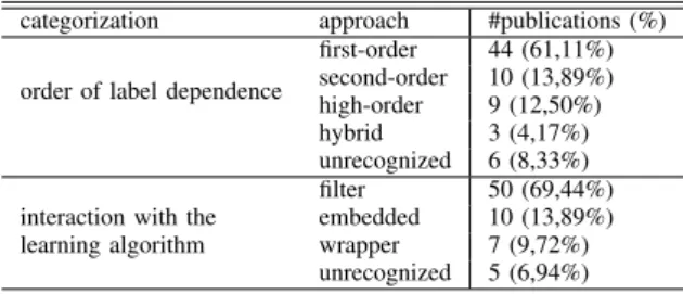
Aiming at capturing a wide, replicable and rigorous overview of the topic, we have instantiated the systematic literature review process [6] for multi-label FS in [7], and re-cently updated it in [8]. TableIIsummarizes the 72 publica-tions found in terms of the two categorizapublica-tions described in SectionII: order of label dependence and interaction with the learning algorithm. The 72 references are listed in the sup-plementary material available athttp://www.labic.icmc.usp. br/pub/mcmonard/ExperimentalResults/BRACIS2014.pdf.
Table II
NUMBER OF RELATED PUBLICATIONS PER APPROACH(total 72) categorization approach #publications (%) order of label dependence
first-order 44 (61,11%) second-order 10 (13,89%) high-order 9 (12,50%) hybrid 3 (4,17%) unrecognized 6 (8,33%) filter 50 (69,44%) interaction with the embedded 10 (13,89%) learning algorithm wrapper 7 (9,72%)
unrecognized 5 (6,94%)
As can be observed, filters and first-order strategies have been the most usual choices in multi-label FS. Differently from the 10 second-order approach publications, the pro-posed method, described next, pioneers label construction.
IV. THE PROPOSED METHOD:LCFS
Given a multi-label dataset D with the set of single labels L y1, y2, y3, . . . , yq , the main idea of LCFS is to construct q new single labels by combining the original labels within pairs yi, yj , i j, yi L and yj L. In each iteration,LCFSselects a pair of labels yi, yj fromL and combines the labels within this pair to generate a new labelyij. After repeating this procedureq times, theq new labels are included in the label setL, such that information
1Discretization is applied to numerical features before usingIG.
about pairwise relationships between original labels can be used by the binary relevance approach for feature selection. The LCFS method consists of two steps, each one con-cerned with answering a different question:
1) Selection: which pairs of labels yi, yj should be chosen?
2) Generation: how to combine these labels to generate the new labelsyij?
Figure1illustrates these steps forq 1.
Figure 1. Applying the two steps ofLCFSto constructq 1new labels Thus, settingLCFSinvolves choosing a strategy to select label pairs and a strategy to combine the labels within each pair. An additional parameter is the number of new labels q that will be constructed. In what follows, the twoLCFS
steps are described.
A. Step 1: selection
Given the set of labels L y1, y2, y3, . . . , yq of the dataset D, LCFS chooses q different pairs of labels2
yi, yj ,i j, according to a selection strategy. The idea is that these pairs capture some pairwise relationships between the labels to be considered by feature selection.
LCFS supports different selection strategies, such as the simple Random Selection (RS), as well as, heuristic strate-gies based on the number of instances labelled by each original single label (label frequency). In particular, two strategies considering label frequency are Co-occurrence-based Selection (CS) and related Labels Selection (LS).CS
sorts in descending order label pairs according to the co-occurrencecc,i.e., the number of instances labelled by both labels within a pair, and selects the firstq different pairs. On the other hand,LScounts (1) the number of instances in which the labels within a pair agree,ce, and (2) the number of instances in which the labels within a pair disagree,cd. Then, the pairs are sorted, in descending order, into two lists according to the values ofce andcd. The pair with greatest value is selected, removed from the correspondent list and the procedure is repeated until selectingq different pairs.
B. Step 2: generation
In this step, LCFS combines both labels from all previ-ously selected pairs yi, yj , i j, to construct the new
2In this work, two label pairs are considered different if they do not
labels yij. The idea is that the values of yij represent a pairwise relationship between yi and yj. In the end, all instances inDare labeled by theqoriginal labels and theq new labels. LCFSsupports different combination strategies between binary variables (labels). In this work, we use three simple logical operators to generate the values of the new labels of each instance inD. The logical operators are:
AND :yij 1iffyi yj 1; yij 0 otherwise. XOR :yij 1iffyixyj; yij 0otherwise. XNOR:yij 1iffyi yj; yij 0otherwise.
The AND operator clearly highlights co-ocurring labels. XNOR, also known as the coincidence function, assigns the value 1toyij iff the labelsyi andyj agree, whereas XOR does the opposite.
After generating the q new labels, the traditional BR
feature selection approach can be applied to the dataset now labeled by theqqlabels. Note that, by combiningBRwith
LCFS, any single-label FS algorithm can be applied to the augmented dataset with second-order label information [5]. The LCFS method has been implemented in Mulan3, a
multi-label learning package based on Weka4.
V. EXPERIMENTAL EVALUATION
In this work, we use the lazymulti-label learning algo-rithm BRkNN-b to evaluate the quality of the features se-lected, aslazyalgorithms are sensitive to irrelevant features.
BRkNN-b, which is implemented in Mulan, is an improved
adaptation of the single-label k-Nearest Neighbor (kNN) algorithm to classify multi-label examples [9].
In the experiments, a filter FS approach based on In-formation Gain combined with Binary Relevance (IG-BR) is performed (1) in the dataset with the original set of labels (standard approach) and (2) in the dataset with the original labels and the ones constructed by aLCFSsetting. Regardless of the label set used,IG-BRtransforms the multi-label dataset into single-multi-label datasets, applies IG in each single-label dataset and averages theIGscore of each feature Xj, j 1. . . M, across all labels. The resulting feature ranking sorts the M averaged IG values in descending order [10]. Recall that the labels constructed byLCFS are only used to select features.
Afterwards, the subsets of features X ` X, SXS
10%M,20%M, . . . ,90%M, ranked by each FS method are used to describe the dataset, which is submitted toBRkNN-b. Regarding LCFS, four settings combining different Se-lection (S) and Generation (G) strategies — Sections IV-A
andIV-B— are considered:
LS-X. S:LS,G: XOR or XNOR is chosen based on the lists sorted by the values ofce andcd
CS-A. S:CS,G: AND
RS-A. S:RS,G: AND
3http://mulan.sourceforge.net 4http://www.cs.waikato.ac.nz/ml/weka
RS-X. S:RS,G: XOR or XNOR is randomly chosen Recall that theLS strategy sorts the label pairs based on the values ofceandcd. For a given label pairyi, yj,LS-X applies the XNOR operator to generate the new labelyij if the pair was selected from the list sorted byce; otherwise, it applies the XOR operator.RS-X randomly selects the XOR or XNOR operator. See the supplementary material for an illustrative example.
We set the number of new labels q q2, i.e., every single label is selected once ifq is even, or one single label is left out ifq is odd.
A. Multi-label datasets
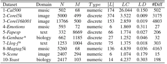
TableIIIsummarizes the characteristics of the 10 datasets used in this work. For each dataset it shows: dataset name (Dataset); dataset domain (Domain); number of instances (N); number of features (M); feature type (T ype); number of labels (SLS); label cardinality (LC), which is the average number of labels associated with each example; label density (LD), which is the cardinality normalized by SLS; and the number of different multi-labels (#Diff).
Table III DATASET DESCRIPTION
Dataset Domain N M T ype SLS LC LD #Diff 1-Cal500 music 502 68 numeric 174 26.044 0.150 502 2-Corel5k image 5000 499 discrete 374 3.522 0.009 3175 3-Corel16k001 image 13766 500 discrete 153 2.859 0.019 4803 4-Emotions music 593 72 numeric 6 1.869 0.311 27 5-Fapesp text 332 8669 discrete 66 1.774 0.027 206 6-Genbase* biology 662 1185 discrete 27 1.252 0.046 32 7-Llog-f* text 1253 1004 discrete 75 1.375 0.018 303 8-Magtag5k music 5260 68 numeric 136 4.839 0.036 4163 9-Scene image 2407 294 numeric 6 1.074 0.179 15 10-Yeast biology 2417 103 numeric 14 4.237 0.303 198
Except for datasets 5-Fapespand8-Magtag5k, the other datasets are available in the Mulan5and Meka6repositories.
In particular,5-Fapespwas built by members of our research laboratory7 [11].8-Magtag5k8 is further described in [12].
Furthermore, 6-Genbase* and 7-Llog-f* are pre-processed versions of the publicly available datasets in which an identification feature and unlabeled examples, respectively, were removed.
B. Results and discussion
First, we compared the learning performance of the classi-fiers built from the datasets described by the features selected by (1) the standardIG-BRapproach and by (2)IG-BRafter applying the fourLCFSsettings to construct the new sets of labels:LS-X,CS-A,RS-AandRS-X.
For each dataset, the number of nearest neighbors k was set as the one that maximizes the Example-based
5http://mulan.sourceforge.net/datasets.html 6http://meka.sourceforge.net/#datasets 7The dataset can be obtained from the authors. 8http://tl.di.fc.ul.pt/t/magtag5k.zip
250
F-measure of the BRkNN-b classifiers built using the original dataset. This value was found in a preliminary study, in which k was varied in the interval 1..27 with step 2 and in the interval 29..99 with step 10. The k values used for each dataset in Table III were 1,59,2,21,3,49,4,15,5,29,6,1,7,13,8,
17,9,27,10,21. All the remaining parameters related to classification and FS were executed with default values. Note that this experimental setup clearly favours the classifiers built using the original datasets.
For each evaluation measure described in Section II-A2
and estimated according to the 10-fold cross-validation strat-egy, the results for IG-BR in the original datasets, as well
asIG-BRin the datasets augmented by using the fourLCFS
settings considering10%up to90%of the features selected (5 FS methods 9 number of features 45 cases) were tabulated. Due to lack of space, this information is available in the SM. For the sake of completeness, we also include in these tables the performance of theBRkNN-b classifiers built using All Features (AF),i.e., without feature selection, as well as, the results of a baseline multi-label classifier namedGeneralB [13].
Although most of the classifiers built using the selected features are better than GeneralB, no FS method was significantly better in terms of each evaluation measure used in this work and number of selected features SXS. In fact, when using the Friedman’s statistical test [14] under the null hypothesis, which states that the performance of the classifiers built after FS are equivalent, the hypothesis is not rejected (significance level α 0.05). Nevertheless, the average rankings calculated by the Friedman’s test give us information about the best method across the datasets — TableIV. In this table, each symbol identifies a FS method: (IG-BR), (LS-X),o(CS-A),(RS-A) and(RS-X).
Table IV
BESTFSMETHOD BASED ON THE AVERAGE RANKINGS
SXS 10% 20% 30% 40% 50% 60% 70% 80% 90%
F-measure o
Hamming loss o
Accuracy o
Fb o
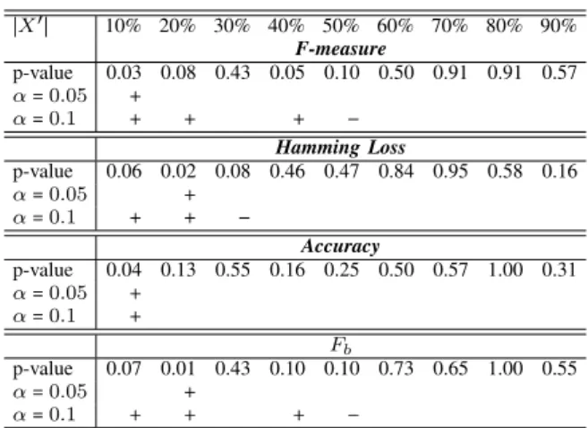
As can be observed,RS-Xoften achieves the best average rankings, specially when SXS @ SX2S, i.e., less than half of the features are used, whereas the standard IG-BR comes next. Thus, we decided to focus on the comparison of both methods. We applied the Wilcoxon signed-ranks test, recommended for comparisons of two algorithms [14], with the null hypothesis that both methods are equivalent. TableV
shows the p-value for each evaluation measure and number of selected featuresSXS, as well as the best FS method when the null hypothesis is rejected (α 0.05and0.1).
Regardless of the evaluation measure, the classifiers built using the features selected by IG-BR in the datasets
aug-Table V
WILCOXON STATISTICAL TEST RESULTS:IG-BR()VSRS-X()
SXS 10% 20% 30% 40% 50% 60% 70% 80% 90% F-measure p-value 0.03 0.08 0.43 0.05 0.10 0.50 0.91 0.91 0.57 α 0.05 α 0.1 Hamming Loss p-value 0.06 0.02 0.08 0.46 0.47 0.84 0.95 0.58 0.16 α 0.05 α 0.1 Accuracy p-value 0.04 0.13 0.55 0.16 0.25 0.50 0.57 1.00 0.31 α 0.05 α 0.1 Fb p-value 0.07 0.01 0.43 0.10 0.10 0.73 0.65 1.00 0.55 α 0.05 α 0.1
mented by using RS-X are significantly better when the number of features is small (13 cases: 4 forα 0.05and 9 forα 0.1). However, the classifiers built using the features selected directly byIG-BRachieve significant improvement in only 3 cases for α 0.1. These results show a clear advantage ofRS-X when the number of features selected is small, which is the aim of FS. Furthermore, comparing to
IG-BR, the increase in complexity of RS-X is only related
to the cost of using XOR or XNOR to generate the set of new labels, as the selection of the label pairs is random.
By outperforming IG-BR, which also aggregates the IG
scores of each feature by averaging them across all labels, in small subsets of selected features,RS-Xcould be related to previous work which compares different aggregation strate-gies in the original set of labels [10]. This work suggests that the averaging strategy is a good choice when the number of selected features is small.
Up to now, we have compared the performance of the classifiers built byBRkNN-b using the features selected by
IG-BR in the original datasets and IG-BR in the datasets
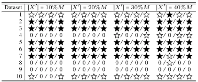
augmented by using the four settings ofLCFS. In this com-parison, RS-X shows better behavior when fewer features are selected. However, the quality of the classifiers have not been taken into account. To this end, we compare the performance of the classifiers built by BRkNN-b, using up to 40% of the features selected by IG-BR in the datasets augmented by using RS-X, with the performance achieved by theBRkNN-bclassifiers using All Features (AF),i.e., the original dataset. Table VIshows, for each dataset, and for each one of the four evaluation measures,i.e.,F-measure/ Hamming loss/ Accuracy/ Fb, whenever the classifiers built using the features selected by IG-BR in the datasets augmented by RS-X have evaluation measure values better than or equal to (indicated byÍ), or at most5%worse than the ones of the classifiers using AF (indicated by ). The symbol0indicates the other cases.
Table VI
CLASSIFIERS BUILT USING THE FEATURES SELECTED WITH THE AID OF RS-X vsTHE CLASSIFIERS BUILT USING ALL FEATURES Dataset SXS 10%M SXS 20%M SXS 30%M SXS 40%M 1 /// /// /// /Í// 2 Í/Í/Í/Í Í/Í/Í/Í Í/Í/Í/Í Í/Í/Í/Í 3 Í/Í/Í/Í Í/Í/Í/Í Í/Í/Í/Í Í/Í/Í/Í 4 0/0/0/0 0/0/0/0 /0/0/ /0// 5 Í/Í/Í/Í Í/Í/Í/Í Í/Í/Í/Í Í/Í/Í/Í 6 Í/Í/Í/Í Í/Í/Í/Í Í/Í/Í/Í Í/Í/Í/Í 7 Í/Í/Í/Í Í/Í/Í/Í Í/Í/Í/Í Í//Í/Í 8 0/0/0/0 0/0/0/0 0/0/0/0 0//0/0 9 0/0/0/0 0/0/0/0 0/0/0/0 0/0/0/0 10 /0/0/ /// /// ///
As can be observed, very good results were obtained in
5out of the10datasets, where the four evaluation measure values of the classifiers based on our proposal are better than or equal to the ones of the classifiers using AF (except for dataset 7-Llog-f*, whereHamming lossis at most5%worse when40%of the features are considered). Good results were obtained in all cases in dataset 1-Cal500, as the results are at most5%worse than the AF ones, whereas there is a very good Hamming loss result when 40% of the features are considered. Similar results are obtained in dataset 10-Yeast
when20%up to40%of the features are considered. Good results were obtained in dataset 4-Emotionsonly when40% of the features are considered (except for Hamming loss). On the other hand, poor results are obtained in datasets
8-Magtag5k and 9-Sceneeven when 40% of the features are
considered. In fact, it is necessary to consider60%and70% of the features selected in datasets 8-Magtag5kand 9-Scene
respectively in order to obtain (///). VI. CONCLUSION
This work proposes LCFS, a method to construct labels to support multi-label feature selection.
Four differentLCFSsettings are compared with the stan-dard approach for FS, which only considers the original label set, in 10 benchmark datasets. The best setting, RS-X, which uses the XOR and XNOR operators to combine labels within pairs randomly selected, gives rise to better classifiers when a small number of selected features (up to
40%) is considered. This shows that constructing labels to support multi-label feature selection is a promising research topic and deserves further attention from the community.
As future work, we plan to evaluateLCFSstrategies based on label weighting [15] and apply Exploratory Data Analysis to understand better the results from specific datasets.
ACKNOWLEDGMENT
This research was supported by the S˜ao Paulo Research Foundation (FAPESP), grant 2011/02393-4.
REFERENCES
[1] H. Liu and H. Motoda,Computational Methods of Feature
Selection. Chapman & Hall/CRC, 2008.
[2] G. Tsoumakas, I. Katakis, and I. P. Vlahavas, “Mining
multi-label data,” inData Mining and Knowledge Discovery
Hand-book, O. Maimon and L. Rokach, Eds. Springer, 2010, pp. 667–685.
[3] K. Lillywhite, D.-J. Lee, B. Tippetts, and J. Archibald, “A feature construction method for general object recognition,” Pattern Recognition, vol. 46, no. 12, pp. 3300–3314, 2013. [4] R. Prati and F. Olivetti de Franca, “Extending features for
multilabel classification with swarm biclustering,” in IEEE
Congress on Evolutionary Computation, 2013, pp. 2964– 2971.
[5] M.-L. Zhang and Z.-H. Zhou, “A review on multi-label
learning algorithms,”IEEE Transactions on Knowledge and
Data Engineering, vol. 99, pp. 1–59, 2013.
[6] B. A. Kitchenham and S. Charters, “Guidelines for perform-ing systematic literature reviews in software engineerperform-ing,” EBSE-2007-01 Technical Report. 65 pg., 2007, Evidence-based Software Engineering.
[7] N. Spolaˆor, M. C. Monard, and H. D. Lee, “A systematic review to identify feature selection publications in multi-labeled data,” ICMC Technical Report No 374. 31 pg., 2012, University of S˜ao Paulo.
[8] N. Spolaˆor, E. A. Cherman, M. C. Monard, and H. D.
Lee, “ReliefF for multi-label feature selection,” inBrazilian
Conference on Intelligent Systems, 2013, pp. 6–11.
[9] E. Spyromitros, G. Tsoumakas, and I. Vlahavas, “An em-pirical study of lazy multilabel classification algorithms,” in Hellenic conference on Artificial Intelligence. Springer-Verlag, 2008, pp. 401–406.
[10] N. Spolaˆor and G. Tsoumakas, “Evaluating feature selection
methods for multi-label text classification,” inBioASQ
work-shop, 2013, pp. 1–12.
[11] R. G. Rossi and S. O. Rezende, “Building a topic hierarchy
using the bag-of-related-words representation,” inSymposium
on Document Engineering, 2011, pp. 195–204.
[12] G. Marques, M. A. Domingues, T. Langlois, and F. Gouyon,
“Three current issues in music autotagging,” inConference
of the International Society for Music Information Retrieval, 2011, pp. 795–800.
[13] J. Metz, L. F. Abreu, E. A. Cherman, and M. C. Monard, “On the estimation of predictive evaluation measure baselines for
multi-label learning,” inAdvances in Artificial Intelligence
-IBERAMIA 2012, ser. Lecture Notes in Computer Science, J. Pav´on, N. D. Duque-M´endez, and R. Fuentes-Fern´andez,
Eds. Springer, 2012, vol. 7637, pp. 189–198.
[14] J. Demˇsar, “Statistical comparison of classifiers over multiple
data sets,” Journal of Machine Learning Research, vol. 7,
no. 1, pp. 1–30, 2006.
[15] S. Jungjit, A. A. Freitas, M. Michaelis, and J. Cinatl, “Two extensions to multi-label correlation-based feature selection:
A case study in bioinformatics,” inIEEE International
Con-ference on Systems, Man, and Cybernetics, 2013, pp. 1519– 1524.
252