Changes in the Berg River Basin over time

(1)

By

Rozwivhona Faith Magoba

Dissertation presented for the the degree of

Doctor of Philosophy (Conservation Ecology)

at

Stellenbosch University

Department of Conservation Ecology and Entomology,

Faculty of AgriSciences

Supervisor:

Professor Karen Esler

Co-supervisor: Professors Cate Brown and Dominic Mazvimavi

(2)

i

Declaration

By submitting this dissertation electronically, I declare that the entirety of the work contained therein is my own, original work, that I am the sole author thereof (save to the extent explicitly otherwise stated) that reproduction and publication thereof by Stellenbosch University will not infringe any third party rights and that I have not previously in its entirety or in part submitted it for obtaining any qualification.

Date: _December 2018

(3)

ii

Summary

The nature of river ecosystems is influenced by the history of activities in their basins. This dissertation investigated historic changes in the Berg River Basin and their influence on river ecosystem structure. The central assumption was that all activities in a river basin landscape contribute either directly or indirectly to the condition (physical, biological, chemical) of rivers that run through them. It was first necessary to establish what changes had taken place in the river basin over time and this was done in different ways at different spatial scales. Changes in land-use were collated and mapped across the basin since these were considered to influence the river’s flow regime and river channel structure. Predictions were made about how changes in flow and river channel habitat would influence the distribution and abundance of aquatic macroinvertebrates.

A history of land-use changes over the Berg River Basin was explored between four periods, 1955-1965, 1976-1985, 1996-2005 and 2006-2015. The bulk of the dryland crop production was in the lower foothills and lowlands while the upper foothills comprised orchards, vineyards and forestry. From 1955-2015 the extent of agricultural land in the basin declined by half as dryland crops were changed to orchards and vineyards and large tracts of land were left fallow. Over the same period the area under forest declined by 73% and urban areas doubled in size as did the number of farm dams in response to the increased need for irrigation to supply the more water hungry crops. The effects of the changes in land-use, the increase in farm dams and the construction of large dams on the river’s flow regime was investigated next.

Changes in flow were explored at four river gauges along the length of the Berg River up- and down-stream of the two main in channel dams; the Berg River Dam in the Upper Foothills and Misverstand Dam in the Lowlands. In general the changes were more marked at the downstream gauges and the trends were towards increased dry season flows and slightly decreased wet season flows due to release of water from, and capturing of floods by the in-channel dams to meet irrigation demand in the dry season. Flow pattern from early records was better correlated with rainfall than that from the recent record indicating that flow changes were likely to be attributable to anthropogenic effects such as land-use and water resource developments. Both land-use and water resource developments were predicted to have consequences on river channel shape and habitat that was investigated next.

Changes in river channel shape, the extent and composition of the floodplain and riparian area was mapped from aerial photographs at five sites along the Berg River and at five adjacent tributaries. Each site responded differently, which was not unexpected, and reductions in the extent of the channel and riparian area were more severe along the Berg River main stem when compared to the tributaries. Along tributaries no floodplains were discernible at the scale measured, however a decreased in extent over time along the main river except downstream of the Berg River Dam where the floodplain area had increased due to the previously braided channel of 1938 changing to a single thread channel with floodplain and a greater area of sandbanks. Changes in river habitat, such as these, were predicted to

(4)

iii

effect change in the abundance and community structure of aquatic macroinvertebrates, which was investigated next.

The abundance of aquatic macroinvertebrates was studied from the 1950s to 2015 and showed a reduction in simulids and baetids with an increase in the abundance of chironomids, indicating a decline in water quality. Changes in other groups indicated a decline in quality of habitat, for instance a loss of plecopterans that prefer clean gravel beds being replaced by caenids that prefer a sandy channel bottom. In 2015 there were also more groups of invertebrates that are associated with slow-flowing areas and marginal vegetation, which was presumed to have occurred in response to the clearing of woody alien trees from the river banks and the subsequent proliferation of aquatic and marginal plants along the water’s edge.

Data collected for land-use, hydrology, channel and riparian changes, macroinvertebrates were synthesized using BEST (BIOENV and BVSTEP) multivariate statistics in PRIMER to search for high rank correlations between environmental and biological variables. When the environmental variables were tested against the biological variables showed that changes in macroinvertebrates were strongly related to area of plantations, area of undeveloped land, the extent of braiding, maximum 5-day average discharge in the wet season and the daily average volume in the dry season. Environmental variables were most influenced/driven by location (separated into sub-basins) while time was the driving factor for the macroinvertebrates data.

(5)

iv

Opsomming

Die aard van rivier-ekostelsels word deur die geskiedenis van hul aktiwiteite in hul komme beïnvloed. Hierdie studie was ŉ ondersoek na historiese veranderinge in die Bergrivierkom en die invloed daarvan op rivier-ekostelselstruktuur. Die sentrale aanname was dat alle aktiwiteite in die rivierkomlandskap direk of indirek tot die toestand (fisies, biologies, chemies) van riviere wat daardeur vloei, bydra. Eerstens moet bepaal word watter veranderinge in die rivierkom met verloop van tyd plaasgevind het, wat op verskillende maniere teen verskillende ruimteskale uitgevoer is. Veranderinge in grondgebruik is noukeurig vergelyk en oor die kom gekarteer, aangesien dit beskou is as verantwoordelik vir die riviervloeistelsel en rivierkanaalstruktuur. Voorspellings is gemaak oor hoe veranderinge in vloei en rivierkanaalhabitat die verspreiding en oorvloed van watermakro-invertebrate sou beïnvloed.

ŉ Geskiedenis van grondgebruikveranderinge in die Bergrivierkom in vier tydperke, naamlik 1955–1965, 1976–1985, 1996–2005 en 2006–2015, is ondersoek. Die meerderheid droëlandgewasproduksie het in die laer voetheuwels en laaglande plaasgevind, terwyl die boonste voetheuwels uit boorde, wingerde en boswêreld bestaan het. Van 1955 tot 2015 het die omvang van landbougrond in die kom met die helfte afgeneem, aangesien droëlandgewasse na boorde en wingerde verander is en groot landstreke braak gelaat is. In dieselfde tydperk het die bosgebied met 73% afgeneem en stedelike gebiede het in grootte verdubbel, en so ook die aantal plaasdamme in reaksie op die verhoogde vraag na besproeiing om aan die waterhonger gewasse te verskaf. Die gevolge van die veranderinge in grondgebruik, die toename in plaasdamme en die bou van groot damme in die rivier se vloeistelsel is hierna ondersoek.

Veranderinge in vloei is by vier riviermeters teen die lengte van die Bergrivier hoër op en laer af van die twee hoofdamme in die kanaal, die Bergrivierdam in die boonste voetheuwels en Misverstanddam in die laaglande, ondersoek. In die algemeen was die veranderinge meer opvallend by die stroomafmeters en die neigings was na verhoogde droëseisoenvloei en effens verlaagde natseisoenvloei weens die vrystelling van water vanaf en opvangs van strome deur die damme in die kanaal om in besproeiingsbehoeftes in die droë seisoen te voorsien. Die vloeipatroon van vroeë rekords is noukeuriger met reënval as in die vorige rekord vergelyk, en het getoon dat vloeiveranderinge waarskynlik aan antropogeniese gevolge soos grondgebruik en waterhulpbronontwikkeling toegeskryf kan word. Daar is voorspel dat sowel grondgebruik as waterhulpbronontwikkeling gevolge vir rivierkanaalvorm en habitat inhou, wat vervolgens ondersoek is.

Veranderinge in rivierkanaalvorm en die omvang en samestelling van die vloedvlakte en oewergebied is van lugfoto’s by vyf terreine langs die Bergrivier en vyf aangrensende takriviere gekarteer. Al die terreine het verskillend gereageer, wat nie onverwags was nie, en verlaging van die omvang van die kanaal en oewergebied was groter langs die Bergrivier-hoofrivier in vergelyking met die takriviere. Geen vloedvlaktes is langs die takriviere teen die gemete skaal waargeneem nie, alhoewel ŉ afname in omvang met verloop van tyd langs die hoofrivier af waargeneem is, maar wel nie laer af van die Bergrivierdam nie, waar die

(6)

v

vloedvlakte-oppervlakte toegeneem het weens die vorige vlegkanaal van 1938, wat in ŉ enkeldraadkanaal met vloedvlakte en ŉ groter oppervlakte sandbanke verander het. Die voorspelling is gemaak dat veranderinge in rivierhabitat, soos hierdie, verandering in die oorvloed en gemeenskapstruktuur van watermakro-invertebrate teweeg sou bring, wat vervolgens ondersoek is.

Die oorvloed watermakro-invertebrate vanaf die 1950’s tot 2015 is bestudeer en het ŉ afname in simuliede en baetiede getoon, met ŉ toename in die oorvloed chironomiede, wat op ŉ afname in watergehalte dui. Veranderinge in ander groepe dui op ŉ afname in habitatgehalte, byvoorbeeld ŉ verlies aan plekopterane wat skoon gruisbeddings verkies, wat met kaeniede vervang is, wat ŉ sandkanaalbodem verkies. In 2015 was daar ook meer groepe invertebrate wat met stadig vloeiende gebiede en randplantegroei geassosieer word, en die aanname is gemaak dat dit plaasgevind het in reaksie op die uitwissing van houtagtige uitheemse bome aan die rivieroewers en die gevolglike voortplanting van water- en randplante teen die waterrand.

Data wat vir grondgebruik, hidrologie, kanaal- en oewerveranderinge en makro-invertebrate ingesamel is, is met behulp van BEST (BIOENV and BVSTEP) meerveranderlike statistieke in PRIMER gesintetiseer om hooggeklassifiseerde verbande tussen omgewings- en biologiese veranderlikes te vind. Met toetsing van die omgewingsveranderlikes teen die biologiese veranderlikes, is gevind dat veranderinge in makro-invertebrate sterk verband hou met die oppervlakte van plantasies, die oppervlakte van onontwikkelde grond, die omvang van omvlegting, maksimum vyfdag- gemiddelde afloop in die nat seisoen en die daaglikse gemiddelde volume in die droë seisoen. Omgewingsveranderlikes is die meeste deur ligging (in subkomme geskei) beïnvloed/aangedryf, terwyl tyd die dryffaktor vir die data oor makro-invertebrate was.

(7)

vi

Acknowledgements

A heartfelt thank you to my supervisors: Professors Cate Brown and Karen Esler for their undying support, patience and endless guidance through out this period. Their willingness to always share their extensive knowledge and their valued time they spent tierelesly reviewing all my work with constructive criticism and new directions is much appreciated. To the Southern Waters team, thank you for always willing to help, it has been a pleasure working with you; Dr Karl Reinecke for all the headaches I gave you, I know I did. Dr Alison Joubert for literally holding my hand through the hydrology chapter. Ros Townsend thanks for all the life advice. I also thank:

 Water Research Commission for the funding, without which this project would be imposible;

 Bonani Madikizela for his role as the WRC project chairperson and the entire steering committee through out this project;

 Julile Sihlangu for always attending to my map and aerial photo requests at the National Geo-spatial Information centre in Mowbray;

 Prof Adriaan van Niekerk, Zahn Munch and Tristan Stuckenberg for sharing their project data with me;

 Dr Karl Reinecke, Ros Townsend, Lavhelesani Muntswu and Liesl Phigeland for their assistance in the field and laboratory;

 Dr Denise Schael for identification of macroinvertebrate samples to a finer level (species);

 Brunette Katsandegwaza for being a good friend, all those baking and gossip nights. Finally to my beloved family: thank you Ntavheleni Helen Magoba for the constant love and support, you believe in me and always goes an extra mile for me. I love you mom. To my sisters Uhone Sharon and Muofhe Victoria Magoba for being true mothers to my daughter through out my studies, you are a blessing indeed. Lavhelesani Muntswu thank you for being an amaizing partner through out this journey, I will forever cherish you. Lastly all love to my daughter Gudani Muvhoni Muntswu; you are the only thing that kept me going when nothing made sense. Thank you Lord Jesus for enabling me and seeing me through this work.

This dissertation is dedicated to my late father Magoba Ntshavheni Simon for his love for education. I miss you everyday dad.

(8)

vii

C.1. Collation and assessment of data on land-use: Method statement ... 197 C.2. Collation and assessment of hydrological data: Method statement ... 198 C.3. Collation and assessment of channel change and riparian vegetation data: Method Statement ... 199 C.4. Collation and assessment of data from macroinvertebrate surveys: Method Statement ... 200

(11)

x

List of Figures

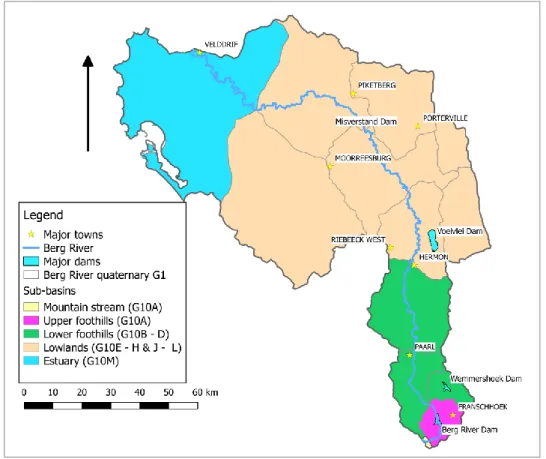
Figure 1.1 Conceptual framework showing processes of the river basin and the four focus areas of the PhD. 1 = large scale land-use changes; 2 = hydrological characteristics; 3 = riparian and channel planform of the river and 4 = aquatic biota (macroinvertebrates) of the basin ... 2 Figure 3.1 The Berg River and its main towns and tributaries. Insert shows a map

of South Africa, the Western Cape Province (grey) and Berg River Basin G1 (red) ... 24 Figure 3.2 Geomorphological zones of the mainstem Berg River, and the

sub-basins that feed each zone ... 25 Figure 3.3 Changes in agricultural land-use classes over time. Top left = land-use

classes for 1955-1965, top right = land-use classes for 1976-1985, bottom left = use classes for 1996-2005 and bottom right = land-use classes for 2006-2015 ... 31 Figure 3.4 Area of total agricultural land, dryland farming, orchards and vineyards,

plantations and urban areas for the whole basin at different time periods. Letters differing between periods indicate significant differences using the Kruskal-Wallis test (p<0.05) (e.g. top left a and b) and where they are the same there is no significant difference (e.g. top right a and a) ... 34 Figure 3.5 ANOVA for differences in distribution of total agriculture land-use

through time. Letters differing between periods indicate significant differences (p<0.05) ... 36 Figure 3.6 Change in area of total agricultural land, dryland farming, orchards and

vineyards, plantations and urban areas between time periods and separated into sub-basins. Letters differing between periods indicate significant differences (p<0.05) (e.g. top left a and b) and where they are the same there is no significant difference (e.g. top right a and a) ... 38 Figure 3.7 Total number of farm dams across the basin ... 39 Figure 4.1 The importance of different parts of the flow regime (after Poff et al.

1997; Bunn and Arthington 2002) ... 43 Figure 4.2 Location of DWA flow gauges on the main Berg River that were

patched for use in the study ... 48 Figure 4.3 The relationship between flow at G1H004 and G1H003 for the period

April 1949 to January 1956 (left). For the period February 1956 to February 1966 (right) ... 50 Figure 4.4 The relationship between flow at G1H004 and G1H020 for the period

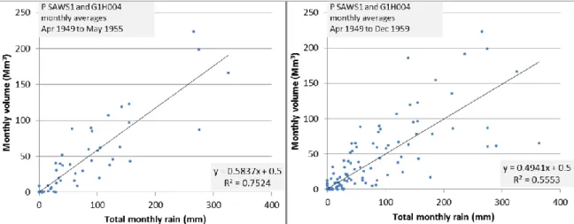
March 1966 to the end of G1H004’s flow record (30 April 2007) ... 50 Figure 4.5 Relationship between rainfall and flow at G1H004 for patching Method

3 for the period 1949 to 1955 (left). The relationship extended to December 1959 (right) ... 51 Figure 4.6 Daily hydrograph for G1H004 showing an extended data gap from

(12)

xi

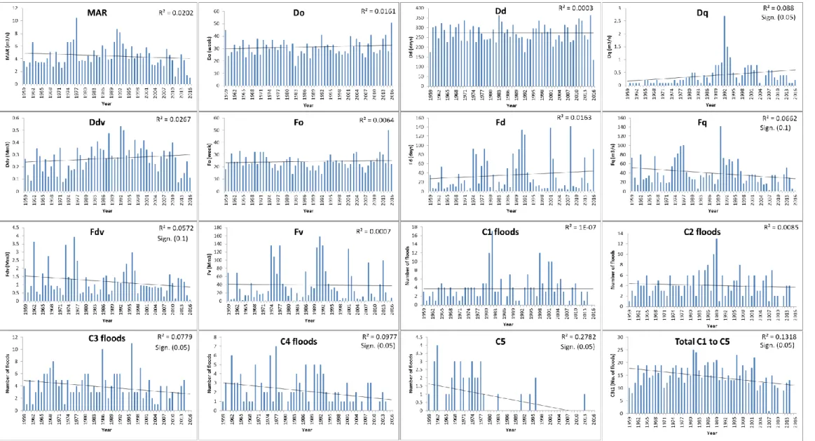
Figure 4.7 DRIFT summary statistics for on the Berg River. Note: There is no difference between the red and blue in the bars in the first graphs ... 55 Figure 4.8 Trends in the DRIFT flow indicators calculated from the data for

G1H004-77 at Bergrivershoek ... 57 Figure 4.9 Trends in the duration of C1 to C5 floods over time (G1H004-77 at

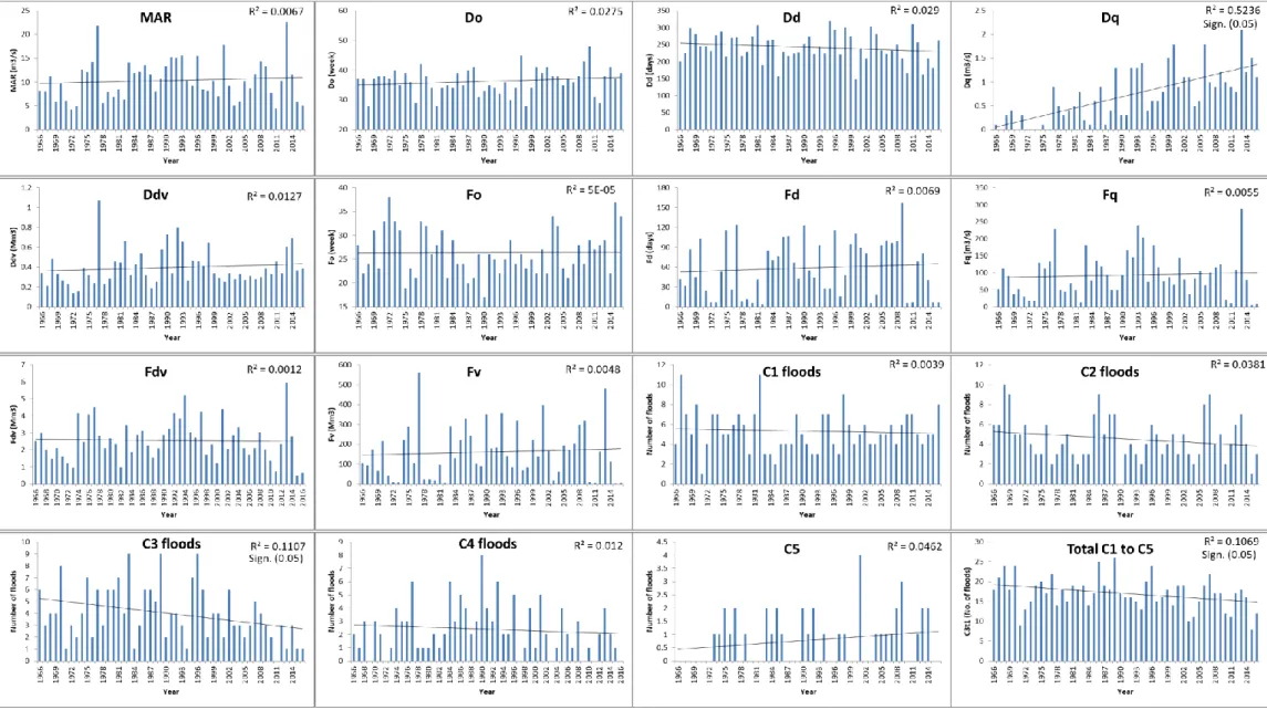
Bergrivershoek (**: p< = 0.05, *, p< = 0.1) ... 58 Figure 4.10 Trends in the DRIFT flow indicators calculated from the data from

G1H020 at Daljosafat ... 59 Figure 4.11 Trends in the duration of C1 to C5 floods over time (G1H020 at

Daljosafat) (**: p< = 0.05, *, p< = 0.1) ... 60 Figure 4.12 Trends in the DRIFT flow indicators calculated from the data from

G1H036 at Vleesbank ... 61 Figure 4.13 Trends in the duration of C1 to C5 floods over time (G1H036 at

Vleesbank) (**: p< = 0.05, *, p< = 0.1) ... 62 Figure 4.14 Trends in the DRIFT flow indicators calculated from the data from

G1H013 at Drie Heuwels ... 63 Figure 4.15 Trends in the duration of C1 to C5 floods over time (G1H013 at Drie

Heuwels) (**: p< = 0.05, *, p< = 0.1) ... 64 Figure 4.16 Double-mass plots of G1H004 MAR against dry season onset (Do), dry

season duration (Dd), dry season volume (Ddv), wet season onset (Fo), wet season duration (Fd), wet season volume (Fdv), the number of Class 3 (C3w) and Class 4 (C4w) and cumulative rainfall ... 65 Figure 4.17 (Left) Periods of change as determined by MAR-DRIFT indicators and

the flow-rain relationship, 3-year average annual volume at G1H004-77, rainfall; (Right) Area of agricultural land-use, and number of dams in the upper foothills... 67 Figure 4.18 (Left) Periods of change as determined by MAR-DRIFT indicators and

the flow-rain relationship, 3-year average annual volume at G1H020, rainfall; (Right) Area of agricultural land-use, and number of dams in the lower foothills ... 72 Figure 4.19 (Left) Periods of change as determined by MAR-DRIFT indicators and

the flow-rain relationship, 3-year average annual volume at G1H036, rainfall; (Right) Area of agricultural land-use, and number of dams in the lower foothills ... 76 Figure 4.20 Differences in Dq before and after the Theewaterskloof-Berg River

scheme and the Berg River Dam completion. Asterisk (*) indicate difference is significant ... 82 Figure 5.1 Example of a flightpath index map from Department of Mapping and

Surveys map with a section of the Berg River between Wellington and Hermon expanded. Flight paths are designated by the vertical lnes with numbered circles. ... 91 Figure 5.2 The location of the reaches (shown as red lines) where data on channel

shape were collected on the Berg River and its tributaries ... 93 Figure 5.3 Images used for Reach 1: Berg River at Franschhoek ... 95 Figure 5.4 Traced images of channel form, sand banks and bars, floodplain and

(13)

xii

Figure 5.5 Traced images of channel form, sand banks and bars, floodplain and

riparian area for the tributary reaches ... 98

Figure 5.6 Channel and riparian, floodplain and sandbank area for the main Berg River reaches for 1938, 2003/6 and 2017 ... 100

Figure 5.7 Braiding and sinuosity for all study reaches for 1938, 2003/06 and 2017 101 Figure 6.1 The location of the 13 study sites in the different sub-basins ... 113

Figure 6.2 CLUSTER analysis of using raw (uncorrected) aquatic macroinvertebrate data from stone (s) and vegetation (v) habitats from sites along the Berg River collected in 1951, 1991 and 2015. Sample codes 9*51v = site 9, 1951, vegetation ... 120

Figure 6.3 CLUSTER analysis of aquatic macroinvertebrate data from stone (s) and vegetation (v) habitats from sites along the Berg River collected in 1951, 1991 and 2015 reduced to the nearest common taxonomic level. Sample codes 9*51v = site 9, 1951, vegetation ... 123

Figure 6.4 CLUSTER analysis of aquatic macroinvertebrate samples collected from stone and vegetation habitats in 1993, 1994, 2003, 2004, 2005 and 2015 ... 127

Figure 6.5 Change in the number of taxa over time for sites that had data for all six years ... 133

Figure 7.1 Map of the study area. Instream Flow Requirement (IFR) sites ... 147

Figure 7.2 MDS showing distribution of the environmental data... 149

Figure 7.3 MDS showing distribution of the biological data ... 149

Figure 7.4 Temporal and spatial resolution for different types of data ... 152

Figure 7.5 The potential use of historic data to inform the calculation of the indices required for REMP, and/or their analysis and interpretation ... 152

(14)

xiii

List of Tables

Table 2.1 Driving concepts of river ecosystem functioning ... 13

Table 2.2 Human activities that have direct/indirect influences on the lotic landscape ... 16

Table 3.1 Geomorphological sub-basins of the Berg River Basin ... 25

Table 3.2 Large dams (> 5000 ML) within the Berg River Basin ... 26

Table 3.3 Definitions of land-use classes ... 28

Table 3.4 Dates of topographic maps used for each period, with bold values indicating years that were patched... 29

Table 3.5 Data used to patch gaps; data from 3319ac and 3318dd were used to construct data for 3319aa ... 30

Table 3.6 Area (km2_{) and percentage of total basin area (%) of each land-use per} sub-basin. Differences between neighbouring periods are shaded ... 32

Table 3.7 Changes in land use between 1955-1965 and 2006-2015, shaded show a decline. For waterbodies only dams are shown. Changes in the other water bodies can be found Appendix Table 8 ... 35

Table 3.8 Rates of change in land-use between the study periods ... 40

Table 4.1 Major water resource developments in the Berg River Basin ... 46

Table 4.2 DWS gauging weirs in the Berg River Basin ... 47

Table 4.3 Gaps that were patched in hydrological records used in the analysis. List excludes gaps shorter than 15 days. Shaded rows indicate the gauges used in the bulk of this chapter ... 47

Table 4.4 Rainfall gauges used ... 49

Table 4.5 Gauges used for patching missing data ... 49

Table 4.6 The ecologically-relevant flow indicators generated using DRIFT software ... 52

Table 4.7 Naturalised and historical MAR (Ractliffe 2009) and historical MAR from this study ... 54

Table 4.8 G1H004-77 data: Periods where inflection points occurred in both flow and rain and in MAR-DRIFT plots, the land-use periods analysed in Chapter 3 and the water-resource periods defined by contruction and operationalization of the major storage dams in the basin ... 68

Table 4.9 The mean values for DRIFT flow indicators for each period at G1H004-77. Highlighted values show where values are significantly different from the following period. Units are given in Table 4.6 ... 68

Table 4.10 Significant differences in aspects of the flow regime between demarcated periods at G1H004-77. Arrow up=significant increase, arrow down=significant decrease while a dash= no significant change ... 69

Table 4.11. Average values of DRIFT indicators for land-use (LU) periods at G1H004-77. Highlighted values show where values are significantly different from the following period. Units are given in Table 4.6 ... 70

Table 4.12. Average values for DRIFT indicators at G1H004-77 before and after the Theewaterskloof-Berg Scheme and the Berg River Dam. Highlighted

(15)

xiv

values are significantly different between the two periods. Units given in Table 4.6 ... 71 Table 4.13 G1H020 data: Periods where inflection points occurred in both flow and

rain and in MAR-DRIFT plots, the land-use periods analysed in Chapter 3 and the water-resource periods defined by contruction and operationalization of the major storage dams in the basin ... 73 Table 4.14 Average values for DRIFT indicators for each period at G1H020.

Highlighted values show where values are significantly different from the following period. Units are given in Table 4.6 ... 73

Table 4.15 Average values for DRIFT indicators for land-use periods at G1H020. Highlighted values show where values are significantly different from the following period. Units are given in Table 4.6 ... 74

Table 4.16 Averages for DRIFT indicators before and after the Theewaterskloof-Berg Scheme and the Theewaterskloof-Berg River Dam at G1H020. Significant differences are highlighted. Units given in Table 4.6 ... 75 Table 4.17 G1H036 data: Periods where inflection points occurred in both flow and

rain and in MAR-DRIFT plots, the land-use periods analysed in Chapter 3 and the water-resource periods defined by contruction and operationalization of the major storage dams in the basin ... 77 Table 4.18 Average values for the DRIFT indicators for each period for G1H036.

Highlighted values show where values are significantly different from the following period. Units are given in Table 4.6 ... 77

Table 4.19 Average values of DRIFT indicators for land-use periods at G1H036. Highlighted values are significantly different from the following period.

(Units in Table 4.6), years in brackets indicate the LU period according to Chapter 3, where the gauged record does not include the full period .... 78 Table 4.20 Average values of DRIFT indicators before and after the Berg River

Dam at G1H036. Highlighted values are significantly different from each other. Units given in Table 4.6 ... 78 Table 4.21 G1H013 data: Periods where inflection points occurred in both flow and

rain and in MAR-DRIFT plots, the land-use periods analysed in Chapter 3 and the water-resource periods defined by contruction and operationalization of the major storage dams in the basin ... 79 Table 4.22 Average values for DRIFT indicators and rain for each period for

G1H013. Highlighted values are significantly different from the following

period. Units are given in Table 4.6 ... 79 Table 4.23 Average values of DRIFT indicators for Chapter 3 land-use (LU)

periods at G1H013. Highlighted values are significantly different from the following period. Units given in Table 4.6 ... 80

Table 4.24 Statistical differences in DRIFT indicators before and after the Theewaterskloof-Berg Scheme, Berg River and Voelvlei Dams at G1H013. Highlights indicate significant differences. Units given in Table 4.6 ... 81 Table 4.25 Correlations between the number of (farm) dams (from Chapter 3) and

(16)

xv

Table 5.1 Aerial surveys that touched on the Berg River available from

Department of Mapping and Surveys (Mowbray) ... 92

Table 5.2 Location of study reaches where detailed data on channel shape were collected along the Berg River ... 92

Table 5.3 Periods analysed for each reach ... 94

Table 5.4 The data extracted from the aerial images for the reaches on the Berg River ... 99

Table 5.5 The data extracted from the aerial images for the tributary reaches ... 99

Table 6.1 Location of study sites and their codes in the different studies, *bolded are dates for actual data collection ... 113

Table 6.2 Methods used to collect macroinvertebrates in the different studies ... 115

Table 6.3 Habitats that were sampled in 2015 for the two methods used (√ = collected, shaded = samples collected from sand, X = habitat absent, grey = sand or mud sampled) ... 116

Table 6.4 Sensitivity weighting for aquatic macroinvertebrates as used in SASS5 scoring system ... 117

Table 6.5 Ecological Categories for interpreting SASS data adopted from Dallas 2007a, South Western Coastal Belt ... 117

Table 6.6 SIMPER analysis of species contributing towards period identity... 119

Table 6.7 Differences in taxonomic resolution and levels at which these were lumped to ensure compatibility across the periods ... 121

Table 6.8 SIMPER analysis of species contributing toward period identity- lumped data ... 123

Table 6.9 SIMPER dissimilarity analysis of taxa contributing toward period separation ... 125

Table 6.10 SIMPER similarity analysis of taxa contributing toward group identity ... 127

Table 6.11 SIMPER dissimilarity analysis of taxa contributing toward period separation ... 129

Table 6.12 Average Score per Taxon (ASPT) and Total SASS score at each site and each sampling period ... 131

Table 6.13 Ecological Category/ condition of study sites over time (after Dallas 2007a) ... 132

Table 7.1 Data sets used in the meta-analysis ... 146

Table 7.2 Time periods of samples allocated to the three time periods in the meta-analysis ... 148

Table 7.3 Results of the BEST analysis ... 150

Table 7.4 Timeline of data available for the Berg River Basin ... 153

Table 10.1 Collation and assessment of data on land-use... 197

Table 10.2 Collation and assessment of hydrological data ... 198

Table 10.3 Collation and assessment of channel change and riparian vegetation data ... 199

(17)

1

Introduction

1.1

Background

River systems run through different landscapes that change over time (Dorava et al. 2001).

Changes in landscapes may be caused by natural/environmental or human beings through modifications of the land-use and land cover. This landscape influences and determines the river’s ecosystems and its overall ecological condition (Naiman et al. 2005). This dissertation

seeks to quantify the links between a river system and the landscapes it drains, by explaining how the physical drivers of river condition (land-use, flow and riparian vegetation) influence the responses of aquatic biota (macroinvertebrates). The need to understand this links is important in order to understand and predict how aquatic biotas (macroinvertebrate) respond to change in surrounding land-use and flow characteristics. This is motivated by the central assumption that all activities that happen within a river basin contribute to the river’s ecological state (Naiman et al. 2005). The intention is that if possible at the end of this

project, the large and small scale information that has been acquired from all chapters can be integrated to furthermore develop a protocol that can be replicated in other river basins through establishing a framework that may be used for monitoring and updating the Ecological Reserve after implementation.

In the past, water resource management in South Africa was largely supply driven and non-ecological in nature (Roux 1999; Stein 2005; Nomquphu et al. 2007). Initially the allocation

of water for the environment was based on the need to reserve minimum flows for survival of specific species of importance (Mazvimavi et al. 2007). In many parts of the world this is still

the case, while in others there is little scientific input concerning the water needs of freshwater ecosystems (Richter et al. 2006). In South Africa, however, the National Water

Act 36 of 1998 (NWA 1998) made provision for the ‘Reserve’, which is defined as: 1) the quantity and quality of water required to satisfy Basic Human Needs (BHN) by securing a basic water supply as prescribed under the Water Services Act 1997 (Act no. 108 of 1997) for people who rely on water from the relevant water resources, and; 2) the quantity, quality and distribution in time of water to protect aquatic ecosystems so as to ensure ecologically-sustainable development and use of the relevant water resources. The latter is referred to as the “Ecological Reserve”.

An Ecological Reserve refers to the quantity and quality of water that is set aside in order to provide for the human basic need and an allocation of water for the aquatic environment (NWA 1998). Data on flow, water quality, aquatic macroinvertebrates, riparian vegetation and other indicators are routinely collected at monitoring sites by Department of Water and Sanitation (DWS) personnel (e.g., River Eco-Status Monitoring Programme (REMP) previously known as the River Health Programme (RHP)). These data are used in a number of management processes, including monitoring the ecological condition of rivers and direct implementation of the Ecological Reserve.

Determination of the Ecological Reserve and other decisions on river basin management are based on a combination of biophysical data that are used in an integrated approach that assesses the physical river conditions in an ecologically-relevant way. These include

(18)

2

consideration of data sets of flow, water quality, aquatic macroinvertebrates, fish, riparian vegetation, habitat and other biophysical parameters that are collected at sites along rivers (Roux 1999; RHP 2004). However, there is a need to reconcile site-specific data in a meaningful way with large-scale processes. Furthermore, broad consideration of issues that influence river ecosystem health are not a routine part of river monitoring and water-recource management (McDonnell 2008). Since the nature of lotic ecosystems within a river basin is largely defined and controlled by the landscapes that surround them, and river health is, at least in part, driven by large-scale processes of water and sediment transported across the lotic landscape (Petts 1994; Dorava et al. 2001; Ward et al. 2001; Naiman et al. 2005), the

landscape approach provides vital context for the evaluation of changes in a river.

The interaction between land, river and elements of the hydrological cycle are illustrated in the lotic landscape (Figure 1.1) and comprise four main habitats; land, the riparian area and floodplain, the river banks and channel, and the hyporheos.

Climate, topography, geology and land-use influence the hydrology of the basin (flow and rainfall), structure and pattern of the channel and its riparia and ecosystem functioning (both aquatic and terrestrial).

Figure 1.1 Conceptual framework showing processes of the river basin and the four focus areas of the PhD. 1 = large scale land-use changes; 2 = hydrological characteristics; 3 = riparian and channel planform of the river and 4 = aquatic biota (macroinvertebrates) of the basin

(19)

3

River ecosystems are defined by, and profoundly affected by changes to, processes within their basins (Dorava et al. 2001; Naiman et al. 2005). The central hypothesis of this

dissertation is that all activities in the lotic landscape contribute either directly or indirectly to a river’s ecological condition, as defined broadly by physical, biological and chemical attributes (Harald et al. 1975; Dorava et al. 2001; Naiman et al. 2005). The cumulative result

of the many impacts may lead to changes in basic structure and function of the riverine-riparian ecosystems resulting in a reduced ability to perform ecological functions (Dopplet et al. 2012). With this in mind, understanding the natural and historic fluctuations within river

ecosystems is essential to provide a context within which data that are generated by monitoring programmes could be assessed. There is a growing awareness to incorporate these large-scale and less-obvious causes of change into judgements made with respect to river condition (Opperman and Harrison 2008; Doppelt et al. 2012). This study enhances our

current understanding of the natural and historic fluctuations within river ecosystems, and their drivers, at a river basin scale through the use of long-term data sets of historic impacts and ecosystem condition. The main aim of the study is to document, analyse and assess large-scale biophysical data that are readily available to help inform monitoring of rivers. The four ovals (Figure 1.1) highlight the four focus areas of the PhD dissertation using the linked elements of the hydrological system on the lotic landscape.

The study was based on the framework that the river basin landscape provides context for the river determined by its geological and climatic properties as well as the historical changes that have taken place. The schematic diagram uses the hydrological cycle to illustrate the river structure and function within the lotic landscape (Figure 1.1). During precipitation water either; infiltrates the soil, is intercepted by vegetation, runs off over land or immediately evaporates (Figure 1.1 - 2: blue oval). The path taken affects the length of time that a water drop spends in the basin and leaches nutrients and minerals from the surrounding rocks and soils, which determine its chemical nature. The length of the journey, and the quality of the water at the end of the journey, are affected by four main, interlinked, variables; climate, geology, topography and the nature and extent of the vegetation cover as well as the human-induced changes (1: green oval). Floods influence the nature and structure of the riparian area and flood plain (see Section 2.1), which in turn influences the structure and character of the bank and bed habitats, and the flow between these (Figure 1.1 - 3: orange oval).

In accordance with the focus areas, five primary objectives of the study were as follows: (1) To document large-scale land-use changes in the lotic landscape over space and time (green oval); this objective was addressed using the green oval by using a broader view that considers the interactions between the river and its surrounding land as water, organic matter, sediments, nutrients and biota move through the river basin. The length of the journey and the quality of the water at the end of the journey, are affected by four main, interlinked, variables; climate, geology, topography, land-use and the nature and extent of the vegetation cover.

(2) To examine the temporal hydrological characteristics of the river basin by analysing the historical hydrology of the Berg River and identify major changes in the volume or seasonal distribution of flow, and where possible identify the underlying causes thereof (blue oval). (3) To identify changes in river channel structure and the riparian area over time and where possible to link these with changes in land-use and flow along the river. The combined

(20)

4

action of all activities that are happening at all parts of the basin are also reflected on the changes of the properties of the channel and its riparian area over time (Figure 1.1 - orange oval).

(4) To identify patterns in aquatic macroinvertebrate communities in the Berg River over time and to compare these to other changes in the basin and river in an effort to identify key drivers of change. The combined action of all activities that are happening at all parts of the basin are also reflected on the changes of the properties of the aquatic biota over time (Figure 1.1 - red oval).

(5) A fifth and overarching objective was to use the insights gained to develop a framework for the collation and evaluation of similar data, as and when available, in other basins with a view to improving the spatial and temporal context within which ecological monitoring data are evaluated. The approach was to build a database of different information layers, such as topography, land-use type, urban development and agricultural areas, hydrology and macroinvertebrates, each representing particular periods in the history of the basin from as early as possible with various time-layers from c. 1900 to 2015.

1.2

Definitions

The following definitions have been applied in this dissertation:

River basin The area of land drained by a river and its tributaries. This can refer to a first order river, a tributary of a larger river or a whole river system (Frissell et al. 1986; Allan et al. 1997).

Lotic landscape The landscape in which lotic aquatic ecosystems occur, define and control almost every facet of their nature and functioning. For this reason, we have referred to the river basin as the ‘lotic landscape’, defined as comprising all parts of the basin - the terrestrial portions plus the lentic and lotic systems that drain them. The lotic landscape comprises the landscape across which water from rain and/or melting snow/ice drains to a single point at a lower elevation, from whence they join another waterbody, such as a lake or the sea (Davies and Day 1998; Finlayson and McMahon 2004).

Land-use Purpose to which the land cover is committed to, encompasses all

kinds of human uses of the basins, including vegetation/crop type, roads, buildings and other catchment hardening, infilling of wetlands, farm dams, major water-resource infrastructure and impoundments, inter-basin transfers, diversions of rivers; it excludes revetments, channelization or canalisation (Clawson 1965; Australian Government Bureau of Rural Sciences, 2006). Environmental Flows Water that is left in a river system, or released into it, for the

specific purpose of managing the ecological condition of that river (King et al. 2003a).

Ecological Reserve Refers to the volume and quality of flow that is reserved for maintenance of the aquatic ecosystems of the water resource (Yang et al. 2009), this also vary depending on the class of the

(21)

5

Resource Quality

Objectives

Are quantitative and qualitative descriptions of the hydrological, chemical, physico-chemical, geomorphological and biological attributes that can be monitored for compliance of the management classes that have been set (Ashton 2012). This includes the volume and timing of flows that are required for the Ecological Reserve (King and Pienaar 2011).

Thalweg The line of the deepest or lowest elevation within the channel which can also be the middle water course (Bakhashab 1996) Riparian zone Refers to areas directly adjacent to the active channel of a water

course or waterbody that support vegetation communities which are distinctly different to neighbouring terrestrial communities (Naiman et al. 2005; Reinecke et al. 2007)

Intra-annual flood Floods with a return period of less than one year Inter-annual flood Floods with a return period of greater than one year Aquatic

macroinvertebrates

Animals without back bone that which live a part of their lives in freshwater biotopes (Machay & Eastburn 1990).

1.3

Chapter overview

The PhD dissertation comprises five data chapters (Chapters 3-7), plus two introductory chapters (Chapters 1 and 2) and a concluding chapter (Chapter 8), as follows:

 Chapter 1: Introduction and motivation for the study

 Chapter 2: Literature Review

 Chapter 3: Historical changes in land-use of the Berg River Basin. This examines large-scale changes in the lotic landscape of the Berg River.

 Chapter 4: Historical changes in the flow regime of the Berg River. This looks at historical hydrology and identifies the causes of major disruptions in either the volume or distribution of flows in the Berg River.

 Chapter 5: Historical changes in channel planform of the Berg River. This examines changes to the riparian area and/or floodplain, river bank and river channel of the Berg River using historical data to analyse changes over time.

 Chapter 6: Historical changes in aquatic macroinvertebrate communities in the Berg River. This examines changes in the macroinvertebrate communities of the Berg River using historical data to analyse changes over time. The analysis will interpret these changes in terms of the habitat changes described in Chapter 5.

 Chapter 7: A proposed framework for the use of historic data to support the River Eco-Status Monitoring Programme. This last chapter syntheses the four data chapters in order to find correlations between the available environmental data (land-use, hydrology, channel and riparian change) and the biological data (macroinvertebrates).

 Chapter 8: Conclusion

There is also a reference list (Chapter 9) and a series of appendices (Appendix A to Appendix C) that contain additional information of relevance to various data chapters. This study was part of a much bigger Water Research Commission “A framework for using historic information to aid monitoring the ecological Reserve”, WRC project No. K5-2345.

(22)

6

2

Literature Review

2.1

Lotic systems

The landscapes in which lotic ecosystems develop, define and control almost every facet of their nature and functioning (Dorava et al. 2001; Naiman et al. 2005). For this reason, the

basin has been referred to as the ‘lotic landscape’, defined as the terrestrial portions of the river basin, plus the lentic and lotic systems that drain them. The lotic landscape comprises the landscape across which water from rain and/or melting snow/ice drains to a lower elevation, ultimately joining another waterbody, such as a lake or the sea (Davies and Day 1998; Finlayson and McMahon 2004). This landscape provides a context for the river, determined by its geological properties, the prevailing climate and the historical changes that have taken place.

Two broad types of aquatic ecosystems can occur in basins: lotic ecosystems, which are dominated by the unidirectional flow of water, and include springs, streams, rivers and portions of wetlands (Fisher et al. 2007), and; lentic ecosystems, where the water does not

have unidirectional flow, such as ponds, marshes and lakes (Chapman and Reiss 1998). They are separate but connected parts of the lotic landscape, through which water, sediments, nutrients and other elements flow, and both are an important part of, and interact closely with, the surrounding lotic landscape (Ward 1989).

The number and size of streams forming the drainage network through this landscape is determined largely by a combination of area, topography, climate and geology (Finlayson and McMahon 2004). Geomorphic and geologic characteristics of basins such as substrates, faulting, rock types and their mineral content affect the quality of the water draining them, as well as the ground-surface water interactions within them (Leopold 1994; Finlayson and McMahon 2004; Bell 2007). Together these characteristics govern the vegetation of their basins (Bendix and Hupp 2000), the spatial and temporal distribution of the water and sediments supplied to a river, and the river’s ability to arrange and transport these, thereby creating the physical habitat on which the biota exist (Poff et al. 1997;

Burgmer et al. 2006). These multiple influences operate at different spatial scales (Allan and

Johnson 1997), with each pair of points in the drainage network connected by a unique one-dimensional path (Rodriguez-Iturbe and Rinaldo 2001). In the rivers, different morphological units, such as mid-channel bars, terraces and lateral bars, support different biotic communities either due to the processes that are active on them (principally flooding) or because of their physical characteristics such as substrate type (Bendix and Hupp 2000). Substrate size and type influences such diverse aspects of the system as porosity, which affects surface-groundwater interchange, availability of nutrients (Sher and Marshall 2003), suitability for penetration by plants roots, and suitability of habitat for spawning and/or refuge. For instance, rivers with unstable substrates usually have low species diversity (Bunn and Arthington 2002) as they are perilous for the small aquatic life that form the basis of the food chain.

Lotic systems interact with their surrounding basins over four dimensions (Amoros et al. 1987

(23)

7

 longitudinally - upstream to downstream progression;

 laterally - across the main channel and riparian area including floodplains;

 vertically - through the hypoheric zone;

 temporally - through time: daily, seasonal and annual changes in river dynamics and ecosystem functioning.

Rivers usually rise in the mountains, either as a springs or seeps and begin their journey to the sea by flowing down steep, narrow channels, with clear fast-flowing water (Davies and Day 1998). Here the beds tend to be coarse with large boulders and rocky outcrops (Finlayson and McMahon 2004; Davies and Day 1998). These upper reaches are the production zone in that they usually generate the bulk of the water and sediments that are transported downstream (Rodriguez-Iturbe and Rinaldo 2001; Finlayson and McMahon 2004). Out of the mountains, in the middle or foothill reaches (Rowntree et al. 2000), the

slope tends to be gentler, and the river bed widens, reducing the flow velocity (Davies and Day 1998). Additional flow is delivered mainly through tributaries. These middle reaches are the transport or transfer zone where both erosion and deposition both take place (Rodriguez-Iturbe and Rinaldo 2001). The water is less pure and more turbid than in the upper reaches (Davies and Day 1998). Out of the foothills, in the lower reaches, the river valley is wider allowing more lateral movement and meandering (Allan and Castillo, 2007), especially on the coastal plain. These lower reaches are predominately the deposition zones (Finlayson and McMahon 2004). Discharge is highest of all the reaches, as increasingly more tributaries join the main river (e.g., Allan and Castillo 2007), but the river slope is flatter and flow velocity drops resulting in sediment deposition (Rodriguez-Iturbe and Rinaldo 2001). The overall the characteristics of a river system in any one of these reaches, however, depends on the transfer of water, sediments, nutrients and organic matter (Petts and Foster 1985), and the interaction and association of river biota is in relation to the nature and conditions imposed by these (Finlayson and McMahon2004). Longitudinal connectivity from upstream to downstream is provided by the channels. For a river channel to form it requires sufficient water discharge and slope to erode and transport surface material (Bridge 2009). Typically, the channel is distinguishable from the surrounding areas by a marked increase in water velocity and, in the lower reaches, by natural leeves (Junk et al. 1989). During the initial

stages of development, channels tend to accommodate to local geography and geological structures, developing along fault zones (Finlayson and McMahon 2004; Bell 2007). However, as water, sediments, and organic debris are routed through the drainage network, channel form is shaped to an ever greater degree by processes that govern the supply and transport of these materials (Montgomery 1999; Kleinhans 2010). For instance, an increase in sediment load with less transport capacity (less water) may result in braided channels whereas a reduction in sediment load may result in meandering of a channel (Church 2006). The width of the channel is also determined by the processes of floodplain formation and destruction (Kleinhans 2010). River channels and their associated riparian areas increase in width and complexity with longitudinal distance from the source as the balance between sediment supply and transport shifts from supply limited channels upstream to transport limited channels downstream. The study of river morphology groups parts of the drainage network according their relationship to their source (Rodriguez-Iturbe and Rinaldo 2001); channels that originate at the source (spring or seep) with no tributaries are called first order

(24)

8

streams; when two first order streams join they form a second order stream and as more streams join the system network the order increases; assuming that when two channels of order N join, they form a channel of order N + 1 (Stahler 1957; Scheidegger 1965). As

tributaries join each other, channel networks arrange in different drainage patterns such as dendritic, trellis, rectangular, radial, angular and parallel (Zernitz 1932). Generally the size of river’s drainage network increases downstream as tributaries and groundwater contribute to flow (Allan and Castillo, 2007). As is the case with the main channel, tributaries have unique characteristics based on the landscapes they drain and the in-channel processes these support (Finlayson and McMahon 2004).

Riparian areas embody the lateral interface between the river channel and the surrounding landscape and comprise a diverse mosaic of landforms, communities and environments within the larger landscape (Naiman et al. 1993; Naiman and Decamps 1997). These areas

are periodically affected by flow and material transfer and, ecologically, are a transition zone between aquatic and terrestrial ecosystems (Jackson and Fisher 1986). Vegetation in these corridors grows in distinct lateral bands, broadly defined by the frequency with which they are inundated (Reinecke and Brown 2013). Where the gradient is gentle, riparian corridors may take the form of floodplains, which are flooded regularly during the wet season by large events that spread out over the area, and then drain back into the channel slowly, often only during the following dry season. As such, floodplain communities are also adapted to seasonal changes in inundation, nutrients, and light (Junk et al. 1989). Since the water on

floodplains is usually slow flowing and/or still, they behave more like lentic than lotic systems (Davies and Day 1998). These are highly productive systems1_{, as nutrients and sediments} from the surrounding basin are carried onto the floodplain by the strongly flowing floodwaters and then left behind by the slow returning flows.

Riparian corridors and floodplains are among the most structurally-complex and biologically-diverse terrestrial landscapes on earth (Lorenz et al. 1997; Ward et al. 2001; Merritt and

Wohl 2002). These are the areas directly adjacent to the wetted channel of a river that support vegetation communities, which are distinctly different from neighbouring terrestrial communities (Reinecke et al. 2007), where the vegetation typically shows a distributional

relationship to the flow regime of the river (Reinecke and Brown 2013). The life cycles of many riparian species have been found to be closely linked to the natural variation of flow of a river (Poff et al. 1997; Friedman and Auble 2000; Pettit et al. 2001). The vegetation zones

themselves occupy a three-dimensional transitional area (longitudinal, lateral and vertical) between aquatic and terrestrial ecosystems and serve as a passageway for the exchange of materials and energy from one ecosystem to the other (Naiman and Decamps 1997; Naiman

et al. 2005; Kondolf et al. 2006; Reinecke et al. 2007; Richardson et al. 2007). The erosional

and depositional forces of floods create different aquatic habitats that are suitable for refuge, spawning and feeding (Aarts et al. 2002), floods also exchange materials (nutrients and

sediments) laterally between the channel and the floodplain.

Healthy riparian areas help to maintain the form of rivers by binding soils and strengthening river banks (Thorne 1990). Trees and shrubs increase channel roughness, thus resistance

(25)

9

to flow, which reduces the velocity of the flow in the channel and may lead to deposition of fine sediments and seeds in these areas (Chaimson 1989; King et al. 2003a). Riparian

vegetation also acts as a buffer against sediments, fertilizers, pesticides and other matter draining from the surrounding landscape through direct chemical uptake (Lorenz et al. 1997;

Dosskey et al. 2010). Riparian areas and floodplains also provide migratory corridors for

animals and breeding; feeding or nursery grounds for a variety of floral/faunal communities (Brode and Bury 1984; Naiman et al. 1993; Corbacho et al. 2003), and provide food and

shelter for people and wildlife.

The vertical interface, between surface and groundwater environments, occurs beneath and alongside a stream bed in an area known as the hyporheos (Vallet et al. 1993; White 1993).

The hyporheic zone is an integral component of rivers, which expands the spatial extent of lotic ecosystem (Ward 1989), and provides critical habitat and refuge for many riverine organisms (Vallet et al. 1993). Here subsurface flows provide nutrients to the river and

surface flows provide dissolved oxygen and organic matter to microbes and invertebrates underground (Stanford and Ward 1993). This zone varies in space and time making it difficult to identify, but the processes and pattern of underflow and discharge depend on proximity of water table to the surface, channel bed permeability, streamflow level, bedrock geology and topography (Boulton et al. 1998; Wiens 2002; Finlayson and McMahon 2004).

In a river basin, the hyporheos tends to be most significant in the middle reaches (Stanford and Ward 1993; Boulton et al. 1998), although floodplains of large alluvial rivers are also

characterized by high volumes of hyporheic flow (Stanford and Ward 1993). Although not much is known about the foodweb dynamics in the hyporheos (Stanford and Ward 1993), the ecosystem consists of interacting physical, chemical, and biological processes (Hakenkamp

et al. 1993; Hendricks 1993; Valett et al. 1993). Different communities of organisms are said

to be interacting within this ecotone, such as insects with hypogean (underground) and epigean (surface) life history stages as well as obligate groundwater species (Stanford and Ward 1993; White 1993). Depending on the bedrock geomorphology water from an unconfined aquifer upwells directly into the channel or floodplain (Stanford and Ward 1993). The spatial and temporal variability inherent in the links between hydrologic, geomorphic and ecological processes are the fourth dimension affecting the nature and functioning of river ecosystems (Montgomery 1999). Flowing water erodes bedrock and soils, and redistributes alluvium (Standford 1998), thus the pattern and variety of flows ultimately determines both the landscape and the nature of the lotic systems draining it as well as the biota it hosts (Poff

et al. 1997). Natural variations in fluvial action (erosion, sediment transport, deposition)

create and maintain a high diversity of morphological units, such as pools, riffles, runs, gravel bars, avulsion channels, islands, debris dams and lateral floodplain terraces (Stanford et al.

1996), making the land-water interface both complex and dynamic (Allan 2004).

The flow regime also exerts direct control over the abundance and spatial arrangement of individuals, their life-history traits and their response to adverse conditions (Poff and Ward 1989; Bunn and Arthington 2002). The flow of water transported sediments through the channel; from uplands through the middle reaches to the lowlands of the basin, the higher uplands are erosion dominated while the lowlands are dominated by deposition (Rodriguez-Iturbe and Rinaldo 2001). Disturbance (floods and intermittency) and flow variability act on

(26)

10

the physical template (Poff and Ward 1989). Flows create and destroy habitats in the channel, in the riparian corridor and on the floodplains (Naiman et al. 1993; Aarts et al.

2002). Flow, in particular floods, also transports plant propagules and nutrients (Friedman and Auble 2000), and provides the medium in which aquatic life can flourish. The flow regime of a river is comprised of different kinds of flow (low and high flow; small, large and larger floods), each of which contributes to the river’s character and maintenance (Dunne and Leopold 1978; Booth and Jackson 1997; Paul and Meyer 2001; Brown and King 2002; Allan 2004):

 Low-flows are the flows in the river outside of floods. They maintain the basic ephemeral, seasonal or perennial nature of the river, thereby determining which animals and plants can survive there. The different magnitudes of low-flow in the dry and wet seasons create more or less wetted habitat and different hydraulic and chemical conditions, which directly influence the balance of species. For instance, species which need to spend several months in water to complete their life-cycles are rare in temporary rivers, though specific riparian tree species may be able to live on such a river’s banks if the groundwater conditions are favourable.

 Small floods occur several times within a year. They stimulate spawning in fish, flush out poor quality water, mobilise sandy sediments, and contribute to flow variability. They re-set a wide spectrum of conditions in the river, triggering and synchronising activities as varied as upstream migration of fish and germination of riparian seedlings.

 Large floods occur more rarely than once a year. They dictate the general geomorphological character, shape and size of a river channel. Floods mobilise sediments and deposit silt, nutrients and seeds on floodplains. They inundate backwater areas, and trigger the emergence of adults of aquatic insects, which provide food for fish, frogs and birds. They maintain moisture levels in the banks that support the trees and shrubs, and prevent the riparian vegetation from being dominated by any one species. Floods also scour estuaries, ensuring, amongst other things, accessibility to marine fish dependent on them as nursery areas, and the maintenance of habitat diversity.

 Larger floods can be catastrophic and costly for both the river system and human life, however they are ecologically important as they reset the system, by altering physical and chemical conditions that influence the long-term development of biotic communities. Extreme droughts and floods are crucial for maintaining common biological, physical characteristics and ecological vitality in rivers (Naiman et al.

2008).

 Flow variability, on a daily, seasonal or annual basis, acts as a form of natural disturbance. This maintains biological diversity through increased heterogeneity of physical habitats. For instance, lack of variability through the absence of small floods may favour fish species adapted to breed under conditions of more constant discharge, with resulting alterations in the relative numbers of fish species and/or loss of native species. Variability in low-flows dictates the width of the vegetation belt along the water line, which protects the banks against erosion. A loss of variability results in a narrowing of this band because the lower portion is no longer regularly exposed or the upper portion regularly inundated. Variability in low-flows dictates the width of the vegetation belt along the water line, which protects the banks against

(27)

11

erosion. A loss of variability results in a narrowing of this band because the lower portion is no longer regularly exposed or the upper portion regularly inundated. Thus, together these flows affect channel configuration, habitat provision and a host of other biological processes (Swanson et al. 1982; Poff et al. 1997; Tuner 1998; Friedman

and Auble 2000; Pettit et al. 2001; Naiman et al. 2005; Camporeale and Ridolfi 2006;

Gurnell et al. 2011).

Naturally, a river exists in a state of dynamic equilibrium, able to respond to seasonal and annual fluctuations in climate because its species have different tolerance ranges and so differ in their abundances as conditions change (Brown and King 2002). Thus, at any time there is a mix of species that can cope efficiently with prevailing conditions, while other species may be present in lower numbers or surviving as, for instance, eggs, seeds or spores, until more suitable conditions occur. The mix of species and numbers of individuals present usually result, in the natural situation, in assemblages where no one species proliferates to “pest” proportions.

Thus, together these flows affect channel configuration, habitat provision and a host of other biological processes (Swanson et al. 1982; Poff et al. 1997; Tuner 1998; Friedman and Auble

2000; Pettit et al. 2001; Naiman et al. 2005; Camporeale and Ridolfi 2006; Gurnell et al.

2011). For instance, Ewart-Smith (2012) found that seasonal variations in the flow regime explained 95% of changes in periphyton biomass and community composition, thereby showing that this temporal variability is exerted even at the very base of the food chain. The size and type of substrate also has bearing on the species able to inhabit a particular area, e.g., a relatively uniform substrate will be favorable for a particular type of community and be a disadvantage to the other communities (Allan 1995, King and Schael 2001). Allan (1995) reported decline of diversity and abundance of macroinvertebrates with stone sizes (cobbles). Resh and Rosenberg (1995) found that larger substrata hosted different species than those found on smaller substrata. Suspended sediment also plays a major role in aquatic systems (Bredenhand 2005), and typically high silting decreases diversity and growth (Chutter 1998). Flow parameters such as water velocity; water as a medium and current as a force strongly determine distribution of biota (Allan 1995). Riparian vegetation plays an important role in dynamics of aquatic body and influences processes and community of the system (Vannote et al. 1980).

Frissell et al. (1986) proposed a hierarchical framework for river habitat classification that

emphasises the river’s relationship to its basin across space and time; from micro habitats, riffles, a connection of pools, tributaries to an entire network of channels (Lorenz et al. 1997).

Within this hierarchy, Petts (1994) described river systems as three dimensional systems, driven by hydrology and fluvial geomorphology; structured by ecosystem food-webs; characterized by spiraling processes (processing of organic matter along the river length); and dependent on change, such as changing flows, moving sediments and shifting channels. Several major and influential concepts have been proposed to explain how these interact to drive ecosystem functioning.

(28)

12

In line with this hierarchy, in South Africa, geomorphological river zones are identified predominantly on the basis of valley form and slope (Rowntree et al. 2000), which tend to

drive many of the other features. The source zone is short and lo