Incremental Figure-Ground Segmentation using
localized adaptive metrics in LVQ
Alexander Denecke1,2, Heiko Wersing2, Jochen J. Steil1, and Edgar K¨orner2 1 Bielefeld University - CoR-Lab, P.O.-Box 10 01 31, D-33501 Bielefeld, Germany
[email protected] http://www.cor-lab.de
2 Honda Research Institute Europe, Carl-Legien-Str. 30, D-63073 Offenbach/Main, Germany
Abstract. Vector quantization methods are confronted with a model selection problem, namely the number of prototypical feature represen-tatives to model each class. In this paper we present an incremental learning scheme in the context of figure-ground segmentation. In pres-ence of local adaptive metrics and supervised noisy information we use a parallel evaluation scheme combined with a local utility function to organize a learning vector quantization (LVQ) network with an adap-tive number of prototypes and verify the capabilities on a real world figure-ground segmentation task.
1
Introduction
The appropriate choice of the number of model neurons is a principle problem in vector quantization networks. In particular incremental learning offers a solution to adjust the amount of resources needed versus classification performance to find a tradeoff between representation quality and the avoidance of over-fitting. Vec-tor quantization methods provide a simple algorithmic yet powerful framework with applications, for example in image processing [1] or life-long learning [2,3]. We investigate such methods in the context of online figure-ground segmentation where homogenous image regions are represented by single feature representa-tives. Ideally the dimensionality of the network should represent the meaningful entities in the data. As this problem is ill-posed (subjective), several researchers have addressed this problem with heuristics in supervised or unsupervised set-tings. One main criterion used for unsupervised setups is the distance of the features to their representatives, namely the quantization error. The criterion in Growing Neural Gas [4] (and similar for the Growing Cell structures [2]) aims at a minimization of the quantization error and introduces new prototypes where the quantization error is large, guaranteeing that the introduction of new proto-types reduces this error. Supervised LVQ primarily aims at the minimization of the classification error which offers another source of information. For example Kirstein et al. [3] propose a heuristics to insert new prototypes at the decision boundary using the misclassified data points together with a distance criterion to determine the location for new prototypes.
In this contribution we investigate Generalized Learning Vector Quantization (GLVQ [5]) with adaptive metrics and propose a framework for incremental and online figure-ground segmentation which faces two problems. Firstly the local adaptive metrics complicates distance-based criteria to place new prototypes, where we use the confidence of the classification instead. Secondly the method has to cope with noisy supervised information, that is, the labels to adapt the networks are not fully confident. In particular we address the second problem by using a parallel evaluation method on the basis of a local utility function, which does not rely on global error optimization. After a short problem statement, we describe the overall method to allow incremental learning in the presence of non-confident supervised information together with the criteria to introduce and remove prototypes from the network. Finally we evaluate the method on a real world segmentation task and compare to previous results.
2
Method
2.1 Scenario
Our proposed method addresses the problem of online figure-ground segmenta-tion for object learning and recognisegmenta-tion. The applicasegmenta-tion scenario consists of a human presenter showing objects to a pan-tilt stereo camera system, which is controlled by an attention system [6]. Using the concept of peripersonal space, the depth estimation of the region in front of the system is analyzed with a blob-detection within a specified depth interval (50cm-80cm). The most salient object in front of the system is continuously tracked and centered in view by setting the gaze direction. Additionally a square region of interest (ROI) is defined based on a distance estimate of the tracked blob and normalized to a size ofI × I pixels, where we use I = 144. Both methods assure an approximate invariance to po-sition and size for the incoming stream of images showing the object in front of cluttered background. A first cue for parts of the scene that belong to the object can be derived from depth estimation which we callobject hypothesis. Because extracting 3D information from 2D images in general is an ill-posed problem, the resulting hypothesis is characterized by a partially inconsistent overlap with the outline/region of the object. That is, some regions of the background are indicated as foreground and vice versa. Since the learning and recognition can be improved as the quality of the figure-ground segmentation is enhanced, we follow the concept of hypothesis refinement to derive the significant object parts (according to the underlying image features) from this initial guess. In [1] we investigated methods for object segmentation that use prototypical feature rep-resentatives to model figure and ground. In particular, we used binarized depth hypotheses as a supervised label for the image features to train a classifier for figure and ground with GLVQ. In our previous setup an empirically predefined number of prototypes were used, while the model selection problem was left open.
2.2 Generalized Learning Vector Quantization
From the camera system the following data is available for each frame. A stack of M = 5 feature maps F := {Fix,y|i = 1..M} corresponding to the RGB color and position information of the pixels forms the dataset D :={ξ|ξx,y =
(F1x,y..FMx,y)T,1≤x, y≤ I}, where every pixel defines a feature vector. To take
advantage from the temporal character of the data the features ofT = 2 frames are combined to one dataset. Switching to a new frame effectively replaces 50% (or less if T is increased) of the data from one to another adaptation step. Additionally to the data the hypothesis H is available indicating which pixels belong to foregroundHx,y = 1 or backgroundHx,y = 0 which is used as label
c(ξx,y) :=Hx,yfor the image features. Assume thatHis partially wrong (i.e. only
a small portion of the data is wrongly labeled), the goal is to derive a classifier
Ax,yF,H(ξx,y) for the pixel features that generalizes to the relevant foreground
(object) features.
The method of GLVQ is defined by a network ofN class-specific prototypical feature representatives P := ©wp∈RM|p= 1..N
ª
. For figure-ground segmen-tation a two class setup is used wherec(wp)∈ {0,1} encodes the user assigned
class-membership of every prototype. The goal of the learning dynamics is to find the representatives in feature space to represent the data by minimizing the classification error defined by the functional E[D,P] = Pξx,y∈Dσ(µ(d)) with σ(x) = 1
1+e−x, µ(d) = ddJ−dK
J+dK. Here the variables dJ = d(ξ
x,y,w J) and
dK =d(ξx,y,wK) represent the distance betweenξx,y and the most similar
pro-totypewJfrom the correct class withHx,y=c(wJ) and the distance to the most
similar prototype wK from an incorrect class. Since similarity-based clustering
and classification crucially depends on the underlying metrics, recently several adaptive metrics were proposed [7]. In the most general case the similarity met-rics is extended towards a Mahalanobis metmet-ricsd(ξ,wp) = (ξ−wp)TΛp(ξ−wp),
where the distance computation of the features to the representatives is extended towards a prototype specific M ×M matrixΛp of relevance factors (Localized
Generalized Matrix LVQ, LGMLVQ). In general, using the kernelized distance computation introduces non-linear decision boundaries. As described in Cram-mer et al. [8] this allows for a reduced number of prototypes while achieving a comparable performance to standard LVQ with multiple prototypes.
The prototypeswJ andwK as well as the corresponding relevance factors
ΛJ and ΛK are optimized by means of gradient descent according to E on
10000·T randomly chosen pairs (ξx,y,Hx,y), which is described in more detail
in [1]. Since Λp has to be positive semi-definite to yield a valid metrics, i.e.
d(ξ,wp) = (ξ−wp)TΩpΩpT(ξ−wp) = (ΩpT(ξ−wp))2 ≥ 0, this is assured
by adapting Ωp, where Λp = ΩpΩpT . Additionally, the diagonal elements are
normalize byPMi=1Λi,i= 1. In general the prototypes are kept from one to the
consecutive frame and adapted to the new data.
To segment an image on the basis of such a network, it is partitioned into
N segments (binary maps) Vp ∈ {0,1} by assigning all feature vectors ξx,y
(i.e. pixels of a particular frame) independently to the prototype wp with the
smallest distanced(ξx,y,w
segmentation A (binary map) is combined by choosing the binary maps from the prototypes assigned to the foregroundA=PNp c(wp)Vp. For object learning
and recognition now Ais used instead ofH.
2.3 Incremental Framework
We showed [1] that this method is robust in the presence of the noisyHand the increased model complexity using the adaptive metrics yields an improved seg-mentation quality in absence of over-fitting effects when an appropriate network dimensionality is chosen. Therefore the number of prototypes is an important parameter which determines the performance of the network with respect to run-time and generalization capability. Our main goal is here to adapt the number of prototypes during online processing of the data to use as many prototypes as necessary for the segmentation.
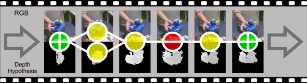
Fig. 1: The general algorithm to adapt the size of the network follows three main parts. Standard adaptation of a network using the LGMLVQ update rules (yellow circles), consisting of step 1 to 3 in Sec. 2.3. The green circles (plus) indicate an additional step to add a new prototype. This step yields two networks which are evaluated in parallel on the consecutive frame. Finally the red circle (minus) indicate an additional contraction step, where one of the prototypes (if appropriate) is removed.
Incremental Online Processing The proposed method consists of three parts, a standard adaptation step, one method to add new prototypes and a local criterion to remove prototypes from the network. To stabilize the incremental learning of the network in presence of the noisy supervised information, we use the temporal aspect of the data for a sequential processing together with a par-allel evaluation scheme. That is, to avoid the adaptation to the hypothesis on a particular frame, adding and removing prototypes are applied in a consecutive manner where on a single frame only one prototype is added or removed. Ad-ditionally due to the risk of disturbing the network with such operations while online segmenting the image, we use a parallel evaluation scheme Fig. 1. The prototypes are added to a second network, which is an exact copy of the first one. After the evaluation a decision is applied whether the original network or the modified network is kept for the following frame.
Controlling the Network Size Incremental learning in prototype-based networks needs a mechanism to control the growing process to determine an appropriate number of prototypes. A widely used possibility is a global quality assessment. This information can be used to select the best performing set of prototypes after the network grew until a predefined maximum number of prototypes was reached [9], or to stop if the change in a quality measure does not significantly vary by adding further prototypes. An online scenario as well as noisy supervised information, which corrupt global quality assessments, prohibits such methods. In our approach the network size is controlled by a local utility function without a criterion of global classification performance or measure for model complexity. In comparison to the work of Hamker [2] we avoid to use (non-normalized) distance-based error criteria for the insertion and removal of prototypes from the network which is attributed to the local metrics of the prototypes. We place new prototypes according to a confidence criterion on the decision boundary and rate this placement afterwards by the utility criterion.
Network Expansion Since a confident global measurement of the representation quality is not available to determine when it is necessary to introduce new pro-totypes the network is expanded in specified time intervals. To decide where a new prototype can be added possible criteria are random insertion, a placement on false classified data or on the decision boundary. In prototype-based networks the decision boundary can be characterized by a similar distance of a feature to two prototypes from different classes. In particular the objective of GLVQ is to minimize an error functional which represents not only the classification error but also introduces an error term for unconfidently classified data points which bases on the difference (the margin) in the nominator of the functionµ(d). Us-ing the margin for learnUs-ing for example was proposed in the context of active learning by Schleif et al. [10]. Here new data points for learning are acquired on the basis of the margin criterion. But this information was not used in the context of incremental learning before. Since the margin is implicitly optimized by the GLVQ error function, we decide to add new prototypes in these regions of low confidence, respectively directly on the decision boundary. Therefore for each expansion step a new prototype is positioned at the training vector with the minimum normalized marginm(ξi) =kdi
J−diKk
di
J+diK . The label of the new prototype is initialized according to the supervised information, while the relevance matrix is taken from the best matching correct prototype according to this label. Since the network size is not adapted on a single frame and the data is changing from one to another frame, adding prototypes does not affect the optimization of the margin but provides a better initialization of the network for the adaptation on the next frame.
Network Contraction To rate the importance of every single prototype in the network a local utility criterion can be used. In the context of vector quantization Fritzke [11] proposes to rate single neurons according to the quantization error of a prototype by the following utility functionU(wp) :=E[D,P \wp]−E[D,P] =
P
ξ∈D kξ−wsk2− kξ−wpk2wherewsis the winning prototype from the set
P \ {wp}. As the quantization error (which is also exploited by Hamker [2] for a
local utility function) is based on a global consistent metrics this method is not appropriate for localized adaptive metrics. Therefore this inspires a utilityu(wp)
function on the basis of the classification error. For a single training exampleξ
this function is:
u(wp,ws, ξ) = (
1 c(wp) =c(ξ), c(ws)6=c(ξ)
0 else
Finally the utility of the prototype on the whole dataset is normalized by the number of activations n(wp) = |{ξ|d(wp,ξ) = min
q∈Pd(wq,ξ)}| of this
proto-type:U(wp) = n(wp1 ) P
ξ∈Du(wp,ws, ξ). If the valueU(wp) falls below a given
thresholdtu= 0.01 in our experiments, the prototype is regarded as a removal
candidate. After an expansion step, the new prototype is kept, if this one and all other current prototypes are useful (i.e. U(wp > tu∀p∈ P)), which assures to
avoid unnecessary instabilities of the network. Independent of the utility function to evaluate the success of an expansion step, we use this function for separate contraction steps of the whole network to determine possibly spare prototypes or misplaced prototypes. Spare prototypes can be replaced by another prototype without impairing the performance. Misplaced prototypes can be characterized by an assignment to the wrongly labeled subset of data by the initial hypothesis
H. Usually this causes in the application/segmentation step that more image portions of the background are assigned to the foreground. These badly placed prototypes can be identified to cause a large classification error even on correctly labeled data and therefore reduce the overall segmentation quality. Together with the recorded activation n(wp) we use the utility criterion to remove such
pro-totypes. That is, additional to the utility criterion a prototype is removed if
n(wp)
|D| < tn, where tn= 0.005.
Algorithm
1. Input and preprocessing:
– feature maps and hypothesis from object ROI:Fx,y :={Fx,y
i |i= 1..M},
Hx,y∈ {0,1}
– Preprocessing of feature mapsF and hypothesisH, see Sec. 3
– Init codebook and metric (on first frame only) P = {wp|p = 1, .., N}
whereN = 2,∀wp ∈ P:wp=|L|1 P
Lξ,L:={ξ|c(ξ) =c(wp)}
– Replace the data of the oldest frame by the data of current feature maps
F in the short term historyD
2. Adaptation (forT update steps)
– Find best matching prototypeswJ for the correct label,wK for the
in-correct label according to a randomly selectedξi∈ D.
e.g.wJ ={wp∈ P|d(wp,ξi) = min
q,c(wq)=Hid(wq,ξ
– Update prototypes wJ,K by means ofwJ,K ←wJ,K+α·∆wJ,K with
learning rate α= 0.05 and similar the relevance factorsΛJ,K with α=
0.005
3. Evaluation: for all pixelsi∈ D
– ∀wp∈ P,Vpi:= (
1 ifd(ξi,w
p)< d(ξi,wr),∀r6=p,{r, p} ∈ P,
0 else
– Determine the binary foreground segmentationA=PNp c(wp)·Vp
– Compute margin for every featurem(ξi) = di J−diK
di J+diK
– Compute utilityU(wp) and prototype activationn(wp), Sec. 2.3 4. (Optional) Network Expansion
– wnew=ξi wherei= arg minξi∈Dm(ξ
i),c(w
new) =Hi,Λnew=ΛJ
– P ={P, wnew},N =N+ 1 5. (Optional) Network Contraction
– selectwpwith the smallest utility p= arg minp∈PU(wp)
– removewp ifU(wp)< tu orn(wp)< tn,P =P \ {wp},N =N−1
3
Results
Data Finally we evaluate the capabilities of this approach on challenging real world image data and investigate the effort of the derived object segmentations in the context of online object learning and recognition. Here we are using the data from [6] consisting of 50 natural, view centered objects with 300 training and 100 testing images. After the acquisition of the feature mapsF and the hy-pothesisHa pre-processingFix,y ←TF(Fix,y) of the feature mapsF
x,y
i (a gamma
correction and white balancing on the maps representing the RGB image data) is performed first. From the available depth and skin information the hypothesis
His computed where all skin-colored areasS,Sx,y∈ {0,1}are removed from the
hypothesisH ←TH(H), where (TH(H) :=H ← H −(H ∩ S)). This is necessary
because the hand is strongly connected to every object/hypothesis and can be regarded as systematic noise violating our assumptions. To compare the results with previous work, the image regions defined by the foreground classification (i.e. the presented objects) are fed into a hierarchical feature processing stage [6]. For object learning and recognition a separate nearest neighbor classifier is ap-plied to the derived high dimensional shape features. The separation of training and test data is used for the object classifier, while the incremental segmentation is adapted on a subset of the pixel data for every single frame.
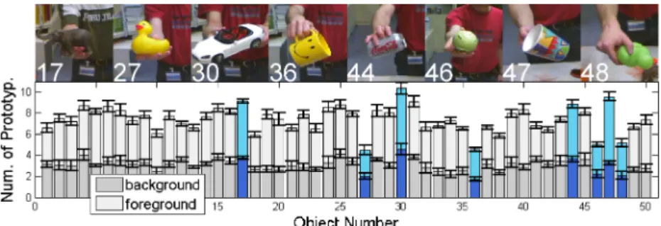
Network Dimensionality First the behavior of the algorithm is analyzed on an example of the training-dataset in Fig. 2. The change in object identity yields an adaptation of the number of prototypes in particular for the foreground, which shows significant differences for some of the objects dependent on their subjec-tive visual complexity. To avoid an influence from the sequence of the presented objects, the order of the 50 objects was randomly rearranged for the eight repe-titions of the experiment. In contrast to previous work a reduced complexity of the representation finally allows for a more efficient processing of single frames.
Fig. 2: Number of prototypes for an application to the training-dataset (50 objects with 300 views, each bar is the average of 8 repetitions and 300 views each). On average over all objects 4.35 prototypes are used for foreground and 3.07 are used for background. Additional the object specific std. dev. of the average number of prototypes for multiple repetitions is drawn, which shows that this number for a particular object is consistent over multiple repetitions of the experiment. On top, examples for eight objects with the highest and lowest number of prototypes are shown.
Classification Performance Compared to a predefined number of prototypes in previous results (see Table 1) three aspects are important: i) the general performance of the object classifier on the basis of the segmentation (an indirect quality assessment, verified in [1]), ii) the used resources to derive the results and iii) the variance in the results. Therefore we compare the incremental method to the results derived by predefined number of prototypes (chosen according to the average number of the incremental method). On the basis of the same resources, a comparable performance can be achieved. Remarkably the variance of the results is significantly decreased which indicates a higher robustness to the noisy supervised data by discarding misplaced prototypes. Together with a faster adaptation to the changing image data the incremental method also reduce the dependency on the initialization of the prototypes. Since the initialization for the fixed prototype setup was purely random this can explain the beneficial effect. Compared to an offline parameter search the incremental segmentation might not be able to reach the potentially maximum performance (for 20 prototypes, 15 background - 5 foreground on this dataset), but offers an application to data with unknown “optimal” number of prototypes.
4
Conclusion
In this paper we present an incremental learning scheme for GLVQ in the context of figure-ground segmentation. In presence of local adaptive metrics and super-vised noisy information we use a parallel evaluation scheme combined with a local utility function to organize a learning vector quantization with an adaptive number of prototypes. On our real world benchmark dataset we show, that the incremental network is capable to achieve a comparable (to the results from [1]) performance in hypothesis refinement while maintaining a significantly smaller
variance of the results, thus is more robust. Due to the parallel evaluation scheme the expansion of the network is free of additional computational load and does not impair the current performance of the network.
N (#bg/#fg) 2(1/1) 7(3/4) 20(15/5) [1] adaptive hypothesis[1] mean 0.7442 0.8715 0.8828 0.8742 0.755 std. dev. 0.0132 0.0110 0.0252 0.0036 n.a.
Table 1: Results of the incremental segmentation scheme compared to previous results (average of 8 repetitions, except the last column). Dependent on the derived num-ber of prototypes (on average 3 for background and 4 for foreground) the proposed method achieves a comparable performance to a predefined prototype setup, whereby the variance of the results is significantly reduced.
References
1. Alexander Denecke, Heiko Wersing, Jochen J. Steil, and Edgar K¨orner. Online figure-ground segmentation with adaptive metrics in generalized LVQ. Neurocom-puting, 72(7-9):1470 – 1482, 2009.
2. Fred H. Hamker. Life-long learning cell structures —continuously learning without catastrophic interference. Neural Networks, 14(4-5):551–573, 2001.
3. S. Kirstein, H. Wersing, and E. K¨orner. A biologically motivated visual memory architecture for online learning of objects. Neural Networks, 1:65–77, 2008.
4. Bernd Fritzke. A growing neural gas network learns topologies. In G. Tesauro, D. S. Touretzky, and T. K. Leen, editors,NIPS, pages 625–632. MIT Press, 1994.
5. A. Sato and K. Yamada. Generalized learning vector quantization. InAdvances in Neural Information Processing Systems, volume 7, pages 423–429, 1995.
6. H. Wersing, S. Kirstein, M. G¨otting, H. Brandl, M. Dunn, I. Mikhailova, C. Goer-ick, J. J. Steil, H. Ritter, and E. K¨orner. Online learning of objects in a biologically motivated visual architecture. Int. J. Neur. Syst., 17(4):219–230, 2007.
7. P. Schneider, M. Biehl, F.-M. Schleif, and B. Hammer. Advanced metric adaptation in Generalized LVQ for classification of mass spectrometry data. InProceedings of 6th International Workshop on Self-Organizing Maps (WSOM), 2007.
8. K. Crammer, R. Gilad-Bachrach, A. Navot, and N. Tishby. Margin analysis of the LVQ algorithm. In NIPS, 2002.
9. A. Jirayusakul and S. Auwatanamongkol. A supervised growing neural gas algo-rithm for cluster analysis. Int. J. Hybrid Intell. Syst., 4(4):217–229, 2007.
10. F. M. Schleif, B. Hammer, and T. Villmann. Margin-based active learning for LVQ networks. Neurocomput., 70(7-9):1215–1224, 2007.
11. B. Fritzke. The LBG-U method for vector quantization – an improvement over LBG inspired from neural networks. Neural Process. Lett., 5(1):35–45, 1997.