A Parallel-In-Time Gradient-Type Method
For Optimal Control Problems
by
Xiaodi Deng
This thesis proposes and analyzes a new parallel-in-time gradient-type method for time-dependent optimal control problems. When the classical gradient method is applied to such problems, each iteration requires the forward solution of the state equations followed by the backward solution of the adjoint equations before the gra-dient can be computed and control can be updated. The solution of the state/adjoint equations is computationally expensive and consumes most of the computation time. The proposed parallel-in-time gradient-type method introduces parallelism by split-ting the time domain into N subdomains and executes the forward and backward computation in each time subdomain in parallel using state and adjoint variables at time subdomain boundaries from the last optimization iteration as initial values. The proposed method is generalized to allow di↵erent time domain partitions for forward/backward computations and overlapping time subdomains.
Convergence analyses for the parallel-in-time gradient-type method applied to discrete-time optimal control problems are established. For linear-quadratic problems, the method is interpreted as a multiple-part splitting method and convergence is proven by analyzing the corresponding iteration matrix. In addition, the connection of the new method to the multiple shooting reformulation of the problem is revealed
and an alternative convergence proof based on this connection is established. For general non-linear problems, the new method is combined with metric projection to handle bound constraints on the controls and convergence of the method is proven.
Numerically, the parallel-in-time gradient-type method is applied to linear-quadratic optimal control problems and to a well-rate optimization problem governed by a sys-tem of highly non-linear partial di↵erential equations. For linear-quadratic problems, the method exhibits strong scaling with up to 50 cores. The parallelization in time is on top of the existing parallelization in space to solve the state/adjoint equations. This is exploited in the well-rate optimization problem. If the existing parallelism in space scales well up to K processors, the addition of time domain decomposition by the proposed method scales well up to K ⇥N processors for small to moderate number N of time subdomains.
I would like to express my gratitude to my advisor Professor Dr.Matthias Heinken-schloss for his continuous support of my Ph.D. research, guidance, and patience.
I also thank the rest of my committee members: Professor Dr.Beatrice Riviere and Professor Dr.John Mellor-Crummey for spending their precious time on my thesis proposal and defense.
I am grateful to my CAAM friends from the bottom of my heart for their company and friendship during these years.
My special thanks also goes to my former undergraduate school friends, Dr.Qu Lu of University of Illinois at Urbana-Champaign, Dr.Lei Huang of National University of Singapore, and Dr. Zheng Fang of University of Illinois at Chicago for many interesting discussions on related research topics.
I really appreciate the great help from CAAM sta↵Daria Lawrence, Brenda Aune, Ivy Gonzalez, Latreece McKinney, and Fran Moshiri. Their compassionate first-class support ensures that I can always focus on my research.
I gratefully acknowledge the sponsors of my research. This work was supported in part by a sponsored research agreement with the ExxonMobil Upstream Research Company and by a 2014 OG HPC Graduate Fellowship administered through the Rice University Ken Kennedy Institute. Part of the computation in this thesis was performed on the Rice University DAVinCI cluster, which was supported in part by the Data Analysis and Visualization Cyberinfrastructure funded by NSF under grant OCI-0959097 and Rice University.
Last but not least, I would like to thank C.C. for her understanding, cheering up, and good temper even when I was often absent-minded at dinner times during the last semester of graduate school. I would like to thank my family for their constant love and unconditional support through all these years from my stepping into elementary
school as a kid at the age of seven to eventually making my way out of graduate school the day before my thirtieth birthday on the other side of the ocean. It has been a long time and the world has changed a lot. But I am so fortunate to be a part of my family that has never changed.
Abstract ii
Acknowledgements iv
List of Figures x
List of Tables xxi
1 Introduction 1
2 Literature Review 8
2.1 Parallel-In-Time Simulation . . . 8
2.2 Parallel-In-Time Optimization . . . 10
2.3 Reservoir Optimization . . . 17
3 Parallel-In-Time Gradient-Type Method in Linear-Quadratic Prob-lems 25 3.1 Gradient Method . . . 26
3.2 Derivation of the Parallel-In-Time Gradient-Type Method . . . 30
3.3 Interpretation as a (2N 1)-Part Iteration Scheme . . . 31
3.4 A Generalized Framework for Parallelism . . . 38
3.4.1 Forward/Backward Computation Subdomains . . . 39
3.4.3 The Algorithm . . . 43
3.4.4 Subdomain Initial/Terminal Processor Rank Function . . . 48
3.4.5 DF and DB . . . . 49
3.4.6 Interpretation as a (DF+DB+ 1)-Part Iteration Scheme . . . 52
3.5 Convergence Proof for the Linear-Quadratic Problems . . . 58
3.6 Numerical Examples . . . 64
3.6.1 1D Boundary Control: Step Size, Non-Monotonic Convergence 66 3.6.2 3D Distributed Control: Parallel Implementation, Strong Scaling 72 3.6.3 1D Distributed Control: Generalized Algorithm . . . 81
3.7 Summary . . . 85
4 Multiple-Shooting Formulations 87 4.1 Continuous Time Multiple-Shooting Formulation . . . 88
4.2 Discrete Time Multiple-Shooting Formulation . . . 90
4.3 Convergence Proof by Multiple-Shooting Formulation . . . 94
4.4 Summary . . . 111
5 Parallel-In-Time Gradient-Type Method in Nonlinear Problems 112 5.1 Metric Projection Properties . . . 115
5.2 Convergence in Constrained Problem . . . 122
5.2.1 Gradient-Type Vector Error Bound . . . 125
5.2.2 Convergence of the Control Update . . . 135
5.2.3 Bound Iterate Around Optimal Control . . . 141
5.2.4 Convergence Theorems . . . 151
5.3 As a Perturbed Gradient Method: Iteration-Wise Monotonicity . . . 158
5.3.1 Iteration-Wise Gradient-Type Vector Error Bound . . . 158
5.3.2 Unconstrained Problem . . . 161
5.3.3 Constrained Problem . . . 168
6 Reservoir Optimization 178
6.1 Introduction . . . 178
6.2 Optimization . . . 180
6.2.1 Example Objective Function . . . 180
6.2.2 Discretized Form of the Optimization Problem . . . 181
6.2.3 Classical Gradient Method . . . 182
6.2.4 Adjoint Equation Approach for Gradient Computation . . . . 183
6.2.5 Projected Gradient Method . . . 183
6.3 Numerical Examples . . . 186
6.3.1 Classical Gradient Method . . . 186
6.3.2 Parallel-In-Time Gradient-Type Method . . . 190
6.3.3 A Heuristic Watchdog Type Parallel Algorithm . . . 203
6.4 Summary . . . 211
7 Conclusions and Outlook 214 Bibliography 218 Appendices 229 A On the Multiple-Shooting Formulation 230 A.1 On the Convergence of the Projected Parallel Gradient-Type Method 230 A.2 Behaviour of Spectral Radius ⇢(I W(↵)) . . . 233
A.3 A Parallel-In-Time Krylov Subspace Based Solver . . . 236
B Reservoir Simulation 244 B.1 Basic Physics . . . 244
B.2 Numerical Scheme . . . 249
B.2.1 Solving Pressure Equation . . . 251
B.3 Trilinos Implementation . . . 256
C Parallel-In-Time Gradient-Type Method Implementation Details In Reservoir Optimization 258 C.1 Algorithms For Explicit/Implicit Formulation of State Equations . . . 259
C.1.1 Gradient Computation with Implicit State Equations . . . 260
C.1.2 Gradient Computation with Explicit State Equations . . . 260
C.1.3 Algorithm with Explicit State Equations . . . 262
C.1.4 Algorithm with Implicit State Equations . . . 262
C.2 Comparison of Algorithms . . . 264
C.3 Application to the Reservoir Problem . . . 269
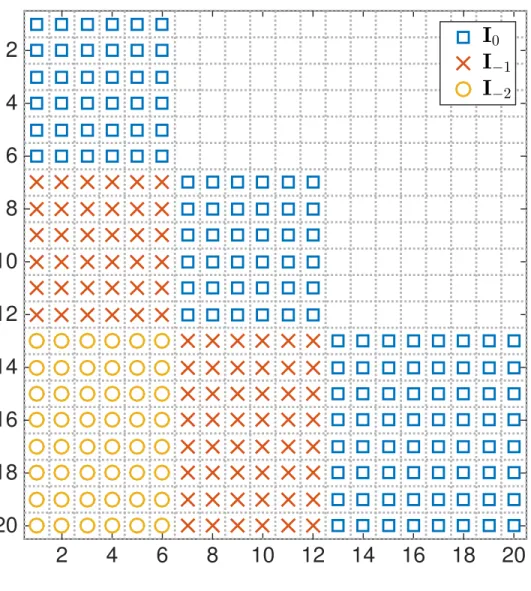
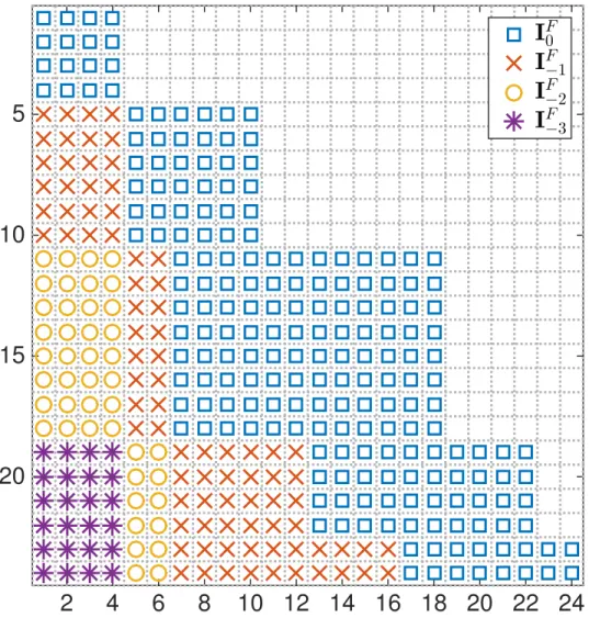
1.1 Workflow of the classical gradient method . . . 2 1.2 Workflow of the parallel-in-time gradient-type method . . . 3 3.1 Illustration of the positions of ‘1’s in I0,I 1 and I 2 in an example
where the state dimension is ny = 2, the K = 10 time steps are split
intoN = 3 subdomains with K0 = 0, K1 = 3, K2 = 6, K3 = 10. . . 36
3.2 Illustration of Generalized Parallel-In-Time Gradient-Type Method. Blue(red) arrows represent time subdomains for parallel forward(backward) computation. The regions in di↵erent processes shaded by the green dots are aggregated and collectively constitute the resulting state/adjoint on the whole time domain for use in subsequent computations. Its time subdomain representation is in Table 3.1. . . 38 3.3 Workflow of One Iteration of the Generalized Parallel-in-Time
Gradient-Type Method Algorithm. Serial computation in central processor is negligible compared to the forward/backward computation happening in the parallel. . . 44 3.4 Illustration of the positions of ‘1’s in IF
0,IF1, IF2, and IF3 in an
ex-ample where the state dimension is ny = 2 and K = 12. The time
domain splitting pattern is illustrated in Figure 3.2 and represented in Table 3.1. Compare with Figure 3.1 for the original parallel-in-time gradient-type method. . . 55
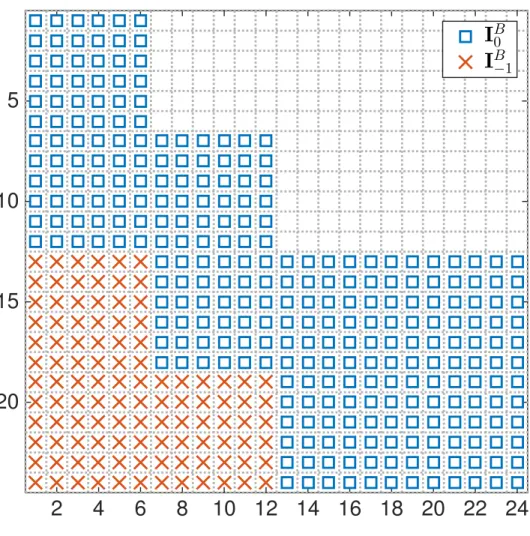
3.5 Illustration of the positions of ‘1’s in IB
0 and IB1 in an example where
the state dimension is ny = 2 and K = 12. The time domain
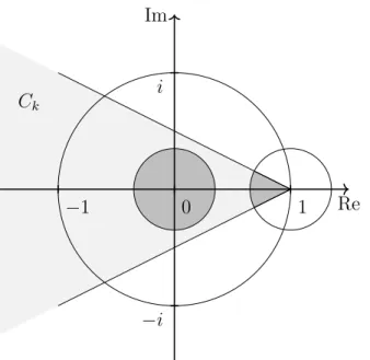
split-ting pattern is illustrated in Figure 3.2 and represented in Table 3.1. Compare with Figure 3.1 for the original parallel-in-time gradient-type method. . . 56 3.6 Eigenvalues of Ce(↵). For sufficiently small ↵ > 0 the eigenvalues
↵ of the companion matrix Ce(↵), defined in (3.5.6) with Pni=0Mi
Hermitian and positive definite, lie in the union of a small open ball around 0 and of the intersection of a small open ball around 1 and the open coneCk, indicated by the dark shaded regions. In particular, all
eigenvalues are inside the unit disk. . . 61 3.7 Speed-ups of the parallel-in-time gradient-type method applied to the
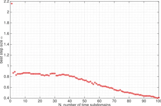
1D optimal control problem. IfI(N) is the number of iterations needed by the parallel-in-time method with N subdomains and cores, the speed-up curve shows I(1)/(I(N)/N). . . 70 3.8 Optimal step-sizes↵for varying numberN of time subdomains for the
1D example problem. . . 71 3.9 Distance between the optimization control variable trajectory and the
optimal control. In this example, 10 time subdomains with optimal step size 0.87 are used. Nonmonotonic convergence is observed and there is a periodic oscillation pattern. Red squares mark the iteration where oscillation reaches its peaks. In this 10 time subdomain case, the peaks happen every 5 iterations on average. See Figure 3.10 for control errors recorded on optimization trajectory on three consecutive peaks. . . 72
3.10 The control error, i.e. the di↵erence between the control in the opti-mization iterations and the precomputed control in the optimal solu-tion, at optimization iteration 44, 49, and 54. They are at the error peaks as depicted in Figure 3.9 as red boxes. Ten time subdomains with optimal step size 0.87 are used. . . 73 3.11 Speed-ups of the parallel-in-time gradient-type method for two
exam-ples problems with end time T = 8 and K = 200 time steps (red curves), and with end time T = 16 and K = 400 time steps (blue curves). For each case two speed-up curves are shown. If I(N) de-notes the number of iterations needed by parallel-in-time method with N subdomains and cores, the speed-up curves indicated by ‘· · · ’ and ‘· · ·+’ show I(1)/(I(N)/N). If t(N) denotes the run time needed by parallel-in-time method with N subdomains and cores, the curves in-dicated by ‘ ⇤’ and ‘ ⇤’ show t(1)/t(N). Excellent speed-ups are obtained for up to N = 20 time domains when T = 8 and K = 200 and for up to N = 50 time domains when T = 16 and K = 400 . The fixed step size for both of the classical gradient method and the parallel-in-time gradient-type method is chosen by trials. The fixed step size with fastest convergence is used. Refer to Table 3.2 and Ta-ble 3.3 for details. . . 76 3.12 Trace graph of 1 second of running time, 8 cores, generated by the
HPCToolkit[ABF+10]. The horizontal axis is the time axis. Eight
horizontal rows represent computation timing of eight cores. The top row is for the first time subdomain, etc. One optimization iteration consists of two major blocks, one purple and one brown. The purple blocks are for forward computation, the brown blocks are for back-ward computation. The smaller green and red blocks correspond to communication and error estimation timing respectively. . . 79
3.13 Trace graph of 1 second of running time, 16 cores, generated by the
HPCToolkit[ABF+10]. The horizontal axis is the time axis. Sixteen
horizontal rows represent computation timing of sixteen cores. The top row is for the first time subdomain, etc. One optimization iteration consists of two major blocks, one shown in purple and the other one shown in brown. The purple blocks are for forward computations and the brown blocks are for backward computation. The smaller green and red blocks correspond to communication and error estimation timing respectively. . . 80 3.14 Control Error History, Test Case 1 in Section 3.6.3.1. . . 82 3.15 Gradient-Type Vector Comparison, Test Case 1 in Section 3.6.3.1. . 83 3.16 Control Error History, Test Case 2 in Section 3.6.3.2. . . 84 3.17 Gradient-Type Vector Comparison, Test Case 2 in Section 3.6.3.2. . 85 4.1 Illustration of direct multiple-shooting optimization variables . . . 88 4.2 Plot of k(I W(↵))kk
2 againstk. In the legend, ⇢((I W(↵)) is also
appended. . . 109 4.3 Ratiok (ˆy(j+1))T,(g(j+1))T,(ˆp(j+1))T k/k (ˆy(j))T,(g(j))T,(ˆp(j))T kagainst
iteration index j. Step size ↵ = 0.01. Random initial ˆy(0), g(0),pˆ(0) is
used. . . 110 5.1 Theorem Dependency Structure in Chapter 5 . . . 114 5.2 Illustration for Lemma 5.1.3, Lemma 5.1.4, and Lemma 5.1.5 on the
relationship between the blue and red lengths and angles. . . 117 5.3 Illustration Lemma 5.1.7. The blue angle is no larger than⇡/2. . . . 122
5.4 Illustration of the first half of the Theorem 5.2.5 proof for the uncon-strained case, i.e.,Dis the whole space and the projectionPD is trivial.
Note that this is a two dimensional illustration of an arbitrary dimen-sional problem. g(i),rJˆ(u(i)), and u⇤ u(i) do not necessarily lie in the
same two dimensional plane. It is typically not true that|✓u ✓˜u|=✓d. 148
5.5 Illustration of the second half of the Theorem 5.2.5 proof for the un-constrained case, i.e., D is the whole space and the projection PD is
trivial. . . 150 6.1 Illustration of a projected gradient step described by Algorithm 15 . . 185 6.2 Location of injection and production wells. Production wells are
indi-cated by crosses; injection are indiindi-cated by circles. Markers connected by solid lines are on the 30 feet layer; markers connected by dotted lines are on the 20 feet layer. . . 187 6.3 Initial well rates (left) and optimized well-rates (right) for the 25
in-jection well and 25 production wells. The color bars with negative well rates above the dashed line in the middle represent the 25 production wells; the color bars with positive well rates below the dashed line in the middle represent the 25 injection wells. The markers (crosses and circles) on the left of each plot are consistent with the markers in Figure 6.2. . . 188
6.4 Contributions of oil revenue (top blue dashed line), water treatment cost (dot-dash red line blow zero), and water injection cost (bottom green dotted line) to the NPV (solid black line) at the initial well-rate settings (left plot) and at the optimal well-rate settings (right plot), for the example problem in Section 6.3.1. Optimization uses the classical gradient method. The area below the black solid line is the NPV. The NPV for the initial well rates (left) is 6.857⇥106; the NPV for the
optimized well rates (right) is 7.986⇥106. A 16.5% improvement is
achieved. The jumps in the curves are caused by the discontinuity in the piecewise constant wells rates. . . 189 6.5 Iteration history of the projected gradient method. After 20 iterations
the optimal NPV is essentially reached and the remaining iterations are used to reduce the norm of the projected gradient below the required tolerance. . . 190 6.6 Contours at day 100, 300, and 500 (final time) of water saturations
resulting from optimized well-rates. Only the bottom half of the reser-voir (depth 20-40 feet) is shown to better display water saturations at the 20 feet level, where several of the wells are located. . . 191 6.7 2D reservoir example, water saturation at day 25. The blue and red
squares mark the injection and production well respectively. . . 194 6.8 2D reservoir example, iteration history of gradient method and the
parallel gradient-type method. The parallel gradient-type method uses 4 time subdomains. . . 194
6.9 Trace graph of about 11 optimization iterations, generated by HPC-Toolkit [ABF+10]. The horizontal axis is the time axis. Four
hori-zontal rows represent computation timing of four cores. The top row is for the first time subdomain, etc. One optimization iteration consists of three major blocks of one purple, one green, and one brown. The purple blocks are for forward computation, the brown blocks are for backward computation, and the green blocks are for waiting. . . 195 6.10 2D reservoir example, optimized well rates at optimization iteration 200.196 6.11 Location of injection and production wells. Circles and crosses are for
injection and production wells respectively. . . 197 6.12 Contours at day 100 and 500 (final time) of water saturations resulting
from optimized well-rates. Only the bottom half of the reservoir (depth 5-10 feet) is shown to better display water saturations at the 5 feet level, where all of the wells are located. . . 198 6.13 3D reservoir example, iteration history of gradient method and
par-allel gradient-type method. Gradient method uses 4 cores in the lin-ear solvers and preconditioners in the forward/backward solves; par-allel gradient-type method uses 4 time subdomains in each of which 4 cores are used in the forward/backward solves, totally, 4⇥4 = 16 cores are computing simultaneously for the parallel-in-time gradient-method. Parallel gradient-type method is initialized by a full gradient sweep and, as a result, the first step takes as long as a serial gradient step. There are vertical red bars on the parallel gradient-type objective values. The other end of bars indicate the infeasible “objective value” computed, for research purpose, during the parallel method runtime using the state variable with jumps at subdomain boundaries. . . 199
6.14 Trace graph of about 10 optimization iterations with evenly split time subdomains, generated by HPCToolkit [ABF+10]. The horizontal
axis is the time axis. From top to bottom, the 16 rows corresponding to 16 cores are grouped into 4 groups. The top 4 horizontal rows represent computation timing of the 4 cores performing parallel computing in the first time subdomain, etc. One optimization iteration consists of three major blocks of one purple, one brown, and one green block. Purple blocks are for forward computation, brown blocks are for backward computation, and green blocks are for waiting. . . 200 6.15 3D reservoir example, optimized well rates at iteration 50. . . 201 6.16 At parallel gradient-type method iteration 50, the 3 dashed lines mark
the position of time subdomain boundaries. As a measure of disconti-nuity, the blue dots are computed by taking the norm of the di↵erence of the states in the current time marching step and the state in the last time marching step. . . 202 6.17 At parallel gradient-type method iteration 160, the 3 dashed lines mark
the position of time subdomain boundaries. As a measure of disconti-nuity, the blue dots are computed by taking the norm of the di↵erence of the states in the current time marching step and the state in the last time marching step. . . 202 6.18 Speed-Up Estimation for Algorithm 16 . . . 207 6.19 Watchdog-Type Algorithm with Suitable Initial Step Size. Initial step
size ↵ = 0.03, inflation factor ⇢inf = 1. Serial Gradient Method is
checking objective decrease condition (Line 19 in Algorithm 16) in each step. The watchdog-type parallel-in-time gradient-type method with Iinner = 10 tests the decreasing condition every Iinner = 10 steps,
6.20 Watchdog-Type Algorithm with Large Initial Step Size. Initial step size↵ = 0.45, inflation factor⇢inf = 1, deflation factor⇢def= 0.5. Serial Gradient Method is checking objective decrease condition (Line 19 in Algorithm 16) in each step. Crosses mark the iterations that fails the objective decrease condition test and thus halves the subsequent step sizes. The watchdog-type parallel-in-time gradient-type method with Iinner = 5 tests the decreasing condition every 5 steps, marked by the
big red circle (pass) or cross (fail). . . 210 6.21 Watchdog-Type Algorithm with Large Initial Step Size. Initial step
size ↵ = 0.45, inflation factor ⇢inf = 1.02, deflation factor ⇢def = 0.5. Serial Gradient Method is checking objective decrease condition (Line 19 in Algorithm 16) in each step. Crosses mark the iterations that fails the objective decrease condition test and thus halves the sub-sequent step sizes. The watchdog-type parallel-in-time gradient-type method with Iinner = 5 tests the decreasing condition every 5 steps,
marked by the big red circle (pass) or cross (fail). . . 212 A.1 Spectral Radius Against Step Size and Number of Subdomains. Two
horizontal axes are for step size ↵ and number of subdomains. The vertical axis is for the spectral radius. A yellow transparent horizon-tal layer is added at z = 1. See Figure A.3 and Figure A.2 for two dimensional slices of this three dimensional plot. . . 234 A.2 Spectral Radius Against Step Sizes. Five curves represent five di↵erent
number of subdomains. . . 235 A.3 Spectral Radius Against Number of Subdomains. Four curves
repre-sent four di↵erent step sizes. . . 237 A.4 sparsity pattern of the HL, N = 4 subdomains, for test case 2 ((3.6.5)
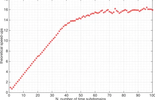
A.5 Performance of the parallel Krylov subspace solver on problem (A.3.2). The red dot represent the serial bench mark. The horizontal axes are number of subdomains. The Top plot shows the number of iterations, I(N), to reduce control error from initial 1e 1 to 1e 12. Theoretical speed-up isN ·I(1)/I(N). Parallel efficiency is I(1)/I(N). . . 240 A.6 Performance of the parallel Krylov subspace solver on problem (3.6.1).
The red dot represent the serial bench mark. The horizontal axes are number of subdomains. The Top plot shows the number of iterations, I(N), to reduce control error from initial 1e1 to 1e 9. Theoretical speed-up isN ·I(1)/I(N). Parallel efficiency is I(1)/I(N). . . 241 A.7 Performance of the parallel Krylov subspace solver on problem (3.6.5).
The red dot represent the serial bench mark. The horizontal axes are number of subdomains. The Top plot shows the number of iterations, I(N), to reduce control error from initial 1e2 to 1e 5. Theoretical speed-up isN ·I(1)/I(N). Parallel efficiency is I(1)/I(N). . . 242 D.1 Time Subdomains Adjustment . . . 272 D.2 Trace graph of 1000 seconds about 8 optimization iterations with evenly
split time subdomains, generated by HPCToolkit [ABF+10]. The
time subdomains are [0,250],[250,500],[500,750],[750,1000] The hor-izontal axis is the time axis. From top to bottom, the 16 rows corre-sponding to 16 cores are grouped into 4 groups. The top 4 horizontal rows represent computation timing of the 4 cores performing parallel computing in the first time subdomain, etc. One optimization iteration consists of three major blocks of one purple, one brown, and one green block. Purple blocks are for forward computation, brown blocks are for backward computation, and green blocks are for waiting. Model problem description in Section 6.3.2.2. . . 273
D.3 Trace graph of 1000 seconds about 9.5 optimization iterations with ad-justed time subdomains, generated by HPCToolkit[ABF+10]. The
adjusted time subdomains are [0,196],[196,442],[442,720],[720,1000] The horizontal axis is the time axis. From top to bottom, the 16 rows corresponding to 16 cores are grouped into 4 groups. The top 4 hor-izontal rows represent computation timing of the 4 cores performing parallel computing in the first time subdomain, etc. One optimization iteration consists of three major blocks of one purple, one brown, and one green block. Purple blocks are for forward computation, brown blocks are for backward computation, and green blocks are for wait-ing. Model problem description in Section 6.3.2.2. . . 274 D.4 Comparison of objective function value history between the
parallel-in-time gradient-type method with di↵erent time subdomain partitions. The evenly split time subdomains are [0,250],[250,500],[500,750],[750,1000]; The adjusted time subdomains are [0,196],[196,442],[442,720],[720,1000]. The first initialization step of a full gradient-sweep is the same for both cases and is not included in the plot. Model problem description in Section 6.3.2.2. . . 275
3.1 Subdomain Representation of Figure 3.2 . . . 41 3.2 T = 8, K = 200 example. Number of iterations and time consumed to
reduce the Infinity-norm control error from the initial guess 1e+3 to 1e-3. Conjugate Gradient method takes only 530 iterations to reach the same level of control error. . . 77 3.3 T = 16, K = 400 example. Number of iterations and time consumed
to reduce the Infinity-norm control error from the initial guess 1e+3 to 1e0. Conjugate Gradient method takes only 340 iterations to reach the same level of control error. . . 78 3.4 Test Case 1 Configuration of Section 3.6.3.1. Total time steps K = 30. 82 3.5 Test Case 1 Configuration of Section 3.6.3.2. Total time steps K = 30. 84 4.1 Notations for the Proof of Lemma 4.3.1. Variables with superscript
“*” are corresponding to the optimal solution. . . 99 5.1 Notations for the Proof of Lemma 5.1.3, Lemma 5.1.4, and Lemma 5.1.5118 5.2 Summary of Lemma 5.2.1 Proof. See the proof for the notations. . . 134 B.1 Nomenclature for the Reservoir Simulation . . . 245 B.2 Nomenclature for the Numerical Scheme of Reservoir Simulation . . 250
Introduction
Optimal control problems governed by a time-dependent partial di↵erential equa-tion (PDE) system are widely studied in various fields of applicaequa-tions, as unsteady fluid-dynamics problems [Gun03], [BLUU12], oil reservoir water flooding optimiza-tion [Jan11], pollutant source inversion [DCZ15], mixing enhancement in microfluidic technologies [HCCT13], etc. Iterative solution of these problems using gradient based methods involve the time consuming repeated solution of a state equation and a so-called adjoint equation. The state equation and adjoint equation of an optimal control problem governed by a time-dependent system are strongly coupled in time and their solution is inherently serial. In other words, the solution of these equations on di↵ er-ent parts of the time domain needs to happen in chronological order, which prever-ents any simple application of parallel computing in the time dimension to accelerate the overall optimization.
To efficiently and rapidly solve these time-dependent optimal control problems by utilizing parallel computing, I propose and analyze a new parallel-in-time gradient-type method (also referred to as “parallel gradient-gradient-type method” in this document). Suppose the PDE is discretized in the space dimension. Let T > 0 be the time domain length and letny, nu 2Z+be the dimension of the state and control variables
respectively at any point in time. For t 2 [0, T], the state is y(t) 2 Rny, the control
Forward State Computation
Backward Adjoint Computation
Update Control
Forward State Computation
Backward Adjoint Computation
Update Control
iter.j
iter.j 1
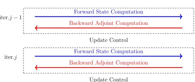
Figure 1.1: Workflow of the classical gradient method
is u(t) 2 Rnu. Let J : Rny⇥Rnu ⇥R ! R and F : Rny ⇥Rnu⇥R ! Rny be given functions. Let ygiven 2Rny be a given initial state. The model problem is in (1.0.1).
min
y,u
Z T
0
J(y(t), u(t), t)dt, (1.0.1a)
subject to d
dty(t) = F(y(t), u(t), t), t2(0, T), (1.0.1b)
y(0) =ygiven. (1.0.1c)
To solve (1.0.1), each iteration of the classical gradient method in reduced control space requires the forward in time solution of the state equation and the backward in time solution of the adjoint equation before the gradient can be computed and the control can be updated. Both of the forward and backward computation is sequential in nature and consumes most of the computation time in the whole optimization process, see Figure 1.1.
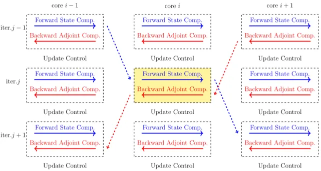
The new parallel-in-time gradient-type method introduces parallelism in the for-ward and backfor-ward computation. In the simplest case, the proposed new parallel gradient-type method evenly splits the time domain into N time subdomains and executes the forward and backward computation in each of the N time subdomains in parallel. To enable the parallelism in N time subdomains, I sacrifice the exact-ness of the gradient vector and aim only for a gradient-type vector surrogate. To
Forward State Comp.
Backward Adjoint Comp.
Update Control
Forward State Comp.
Backward Adjoint Comp.
Update Control
Forward State Comp.
Backward Adjoint Comp.
Update Control
Forward State Comp.
Backward Adjoint Comp.
Update Control
Forward State Comp.
Backward Adjoint Comp.
Update Control
Forward State Comp.
Backward Adjoint Comp.
Update Control
Forward State Comp.
Backward Adjoint Comp.
Update Control
Forward State Comp.
Backward Adjoint Comp.
Update Control
Forward State Comp.
Backward Adjoint Comp.
Update Control
corei 1 corei corei+ 1
iter.j+ 1 iter.j
iter.j 1
Figure 1.2: Workflow of the parallel-in-time gradient-type method
start computations on all time subdomains simultaneously, quantities computed in the last optimization iteration are used as the initial/terminal conditions for the for-ward/adjoint solves, which is readily available for each sumdomain at the beginning of each optimization iteration. This is the key idea of the proposed new parallel-in-time gradient-type method. However, using quantities from last iteration to start parallel computing on subdomains also results in jumps in the state/adjoint variables at time subdomain boundaries. After the state and adjoint variables are computed, the new method uses the same formula as in the classical gradient method to com-pute a gradient-type vector to update the control and begin the next iteration. See Figure 1.2.
In the case where N time subdomains evenly split the time domain, since the length of the forward and backward computation in each time subdomain is 1/N of the original time domain, the computation time for each optimization iteration is expected to be about 1/N of the computing time of the classical gradient method iteration. This is where the parallel-in-time gradient-type method brings potential
speed-ups, if the control update computed in parallel is good enough as a surrogate of the gradient. It is also important to note that the acceleration by parallelism in time multiplies the existing parallelism in the solution of state and adjoint equations. At any iteration of the parallel gradient-type optimization, the state, adjoint, and control variables typically do not satisfy the state equation and the adjoint equation at the time subdomain boundaries as a result of using quantities from the last iteration. Since the new method does not use an exact gradient in the control update, this new method is not an acceleration of the exact classical gradient method and therefore I refer to it as a ‘gradient-type’ method.
I also present a generalization of this newly proposed method that allows the di↵ er-ent time domain partition of the forward and backward computation and overlapping computation domains.
The theoretical analysis consists of results for linear-quadratic problems and the broader class of general non-linear problems.
For convex linear-quadratic discrete-time optimal control (DTOC) problems, the generalized method can be interpreted as a multiple part splitting method (for the N evenly splitted subdomains in forward and backward computation case, it is a (2N 1)-part splitting method [de 76, dN81]) for solving the optimality condition
Hu=g,
whereH is the Hessian, and g is the gradient of the reduced control space objective. However, in the literature, there is not a convergence result applicable to the spe-cific splitting pattern that results from this new method and the existing convergence theorems for the classical gradient method also does not apply since the control up-dates of this method does not use exact gradient. For linear-quadratic problems, I prove the convergence of this new method by using its structure as a multiple part splitting method and spectral radius properties of an implicitly constructed iteration matrix as a block companion matrix [DTW71].
I also study the new parallel-in-time gradient-type method from the point of view of the multiple shooting reformulation of the optimization problem. I show the new method can be seen as using a gradient-type method to solve the saddle point prob-lem of the multiple shooting formulation optimality system. An alternative proof of convergence is given for the linear-quadratic problems using spectral radius type of argument again.
Then, I investigate the behavior of the parallel gradient-type method for general nonlinear optimization problems.Particularly, I consider the projected parallel-in-time gradient-type method whose iteration is the parallel gradient-type iteration appended by a metric projection step that projects the control into a closed convex set. Di↵ er-ent from the spectral radius argumer-ent used in the previous linear-quadratic problem convergence proofs, I use another approach based on the idea that, when the control update is small, the gradient-type vector computed in parallel is similar to the true gradient. I establish a series of theorems and give convergence proofs with di↵erent assumptions on the problem, such as the convexity of the objective function or com-pact control constraints. Additionally, I present results on the monotonic convergence of the method given small step size.
I present numerical examples to demonstrate the proposed method performance. In optimal control problems governed by 3D linear advection-di↵usion-reaction PDE systems, strong scaling is observed in one example with up to 50 cores, i.e., 50 times speed-ups is achieved by the parallelism of 50 cores compared to the serial classical gradient method. Numerical results to demonstrate other properties of the method are also presented.
This work is motivated by an optimization problem arising in the well rate con-trol in the water flooding process of secondary oil reservoir recovery. This is an optimal control problem governed by a system of highly nonlinear time-dependent PDEs. The forward computation, i.e., reservoir simulation, and the backward com-putation is both very comcom-putationally expensive. In this reservoir optimization
prob-lem, the application of the proposed parallel-in-time gradient-type method results in significant speed-ups. In one experiment, 4-time-subdomain parallel gradient-type method with, in each subdomain, 4 cores in the space dimension for parallel linear solvers/preconditioners (16 cores in total) is compared with classical gradient method with 4 cores in the space dimension. About 4 times speed-ups is obtained.
This document is organized as follows. In Chapter 2, I review related work in the parallel-in-time solution of time-dependent systems, parallel-in-time optimization, and oil reservoir optimization. In Chapter 3, I use the linear-quadratic discrete-time optimal control problem to introduce the idea of the parallel-in-time gradient-type method. I first develop a compact notation for the classical gradient method, then derive and reorganize the parallel-in-time gradient-type algorithm into a similar com-pact form which reveals its nature of being a (2N 1)-part splitting method. Then, I generalize the newly proposed method to accommodate flexible overlapping partition of time domains. I prove convergence of the generalized method and demonstrate its performance by numerical experiments, applying the parallel-in-time gradient-type method to 1D and 3D linear-quadratic optimal control problems. In Chapter 4, I in-troduce the direct multiple shooting reformulations of linear-quadratic optimal control problems, which leads to another interpretation of the parallel-in-time gradient-type method.An alternative proof of convergence is given using the multiple shooting per-spective. In Chapter 5, I give convergence proofs and related properties for general nonlinear problems.In Chapter 6, I describe the wellrates optimization problem and compare numerical results of the classical gradient method and the parallel-in-time gradient-type method.
I include several appendices. Appendix A consists of some research without a clear conclusion but still draws insights into the parallel-time gradient-type method, in-cluding discussions on one way of proving the projected parallel gradient-type method convergence, the numerical experiments investigating behavior of the spectral radius of an iteration matrix that determines the convergence speed of the method, and a
parallel-in-time Krylov subspace method that is closely related to the multiple shoot-ing formulation of the linear-quadratic problem. Appendix B describes in detail the impressible immiscible two-phase subsurface flow model PDE and its discretization that is used in the reservoir optimization problem. Appendix C talks about imple-mentation details of the proposed method on the reservoir optimization problem with an emphasis on comparing the parallel-in-time gradient-type method applied to prob-lems with explicit and implicit (as the case of the reservoir problem) expression of state equations. Appendix D presents a test on using a time subdomain partition based on computation load, instead of even number of time steps, for load balance of the parallel-in-time gradient-type method applied to the reservoir optimization problem.
Literature Review
In Section 2.1, I first review some related work on parallel-in-time simulation which give rise to important ideas for parallel-in-time optimization. In Section 2.2, I re-view related literature on parallel-in-time optimization including some commonly used concepts as additive Schwarz preconditioners, direct/indirect multiple shoot-ing formulations of the time-dependent optimal control problems, Parareal [LMT01] based parallel simulation. At last, in Section 2.3, I review related work in the water flooding optimization problem on oil reservoir management.
2.1
Parallel-In-Time Simulation
In [LRSV82], a waveform relaxation family of algorithms was first proposed for an-alyzing nonlinear dynamical system in the time domain. Waveform relaxation is a Gauss-Jacobi type relaxation iterative method. (It can be also Gauss-Seidel type. Because the Gauss-Jacobi type is more straightforward to parallelize, I discuss the Gauss-Jacobi type below.) First, the unknowns are partitioned into spatial subdo-main. Then, in each Gauss-Jacobi relaxation iteration, the algorithm fixes unknowns from all partitions but one and carries out the simulation in time for this one parti-tion of unknowns. A suitable integraparti-tion formula and steps can be applied only to
this partition of unknowns, which allows di↵erent methods to integrate di↵erent un-knowns. The above algorithm constitutes a Gauss-Jacobi relaxation step that can be parallelized and multiple time-dependent simulations can be readily run in parallel. Strictly speaking, this algorithm does not belong to the specific type of parallel-in-time simulation that I discuss here, since it does not perform computation corresponding to di↵erent time subdomains at the same time. But the parallel-in-time gradient-method shares the idea that in one iteration, computation in each partition runs independently with other partitions with essential information from other partitions fixed as quantities computation from the last iteration.
‘Parareal’, an innovative parallel-in-time algorithm for simulation, was proposed in [LMT01]. See also the overview [Gan15]. The method decomposes the time domain into N subdomains and makes use of a coarse(C) and a fine(F) grid time integrator. In the kth iteration, the coarse one integrates over the whole time domain in serial, the fine one integrates each one of the N time subdomain in parallel, and the initial value of each time subdomain is updated by a simple formula (2.1.1) using integration results from the coarse, CTn!Tn+1(Y
(k+1) Tn ), and fine,FTn!Tn+1(Y (k) Tn ), integrations. YT(nk+1+1)=CTn!Tn+1(Y (k+1) Tn ) +FTn!Tn+1(Y (k) Tn ) CTn!Tn+1(Y (k) Tn ) (2.1.1)
AfterN iterations the method produces exactly the same integration result as the fine grid integrator would, but this would not accelerate the simulation. In practice, for many cases, far less than N iterations are needed to achieve desirable error and thus results in lower computation time when executed in parallel. From my point of view, it can be partly seen as making use of the fact that the temporal dependency between states of two time point is decreasing and diminishing as the time distance between these two time increases. Many works based on ‘Parareal’ have been done since the conception of this idea, some of which are reviewed below, e.g. [Com05, DSSS13].
2.2
Parallel-In-Time Optimization
The widely cited paper [TBA86] presents convergence results of a class of distributed asynchronous gradient optimization algorithms. The parallel-in-time gradient-type method does not exactly fall into the category of algorithms discussed in the paper. However, they share the same spirit that, in the case where each processor is com-puting a gradient-like updating step for one component of the optimization variable, the information from other component su↵ers a delay. The convergence theorem and its proof provided in the paper [TBA86] bears significant similarity with the parallel-in-time gradient-type method convergence theorem for non-linear problems that I provide in this dissertation. The first similarity is that convergence is established based on a sufficiently small gradient-type step size whose theoretical upper bound is not particularly tight. If we can trace the proof deductions and find such a upper bound, the upper bound will lead to convergence but not to optimal performance. The second similarity is in the idea of the proof that when the step size is small, the information, i.e. state/adjoint/control, in the distributed system is similar to the information in a virtual centralized system at a specific status, and the gradient-type step made in the distributed system is actually in a descent direction for the information in the virtual centralized system.
The paper [CCL89] presents a method that explicitly decomposes a time-dependent optimal control problem (P) with initial state condition into sub-optimal control prob-lems (P-j) with both initial and terminal conditions on small time subdomains as below (see [CCL89, Equation 2.1-2.5]),
(P) min x,u gN(xN) + NX1 i=0 gi(xi, ui), subject toxi+1 =fi(xi, ui), i= 0, ...N 1, x0 =xgiven, (P-j) min x,u jTX1 i=(j 1)T gi(xi, ui), subject toxi+1 =fi(xi, ui), i= (j 1)T, ...jT 1, x(j 1)T, xjT 1 given.
This method is an iterative method where in each iteration it takes a two level approach. In the lower level, optimal control problems with both initial and terminal state constraints are solved exactly assuming feasibility. Note that feasibility with both initial and terminal constraints is not trivial for many applications. In the higher level, the initial and terminal state values of each time subdomain are updated, e.g., by a Newton step using first and second order information from the lower level. This method shares a similar spirit with indirect multiple shooting method in the sense that in the higher level of both methods variables at the time subdomain boundaries representing initial/terminal values of states/adjoints are updated and the control u in the original problem is updated on the lower level. But there is an apparent di↵erence in how they make use of the information from the lower level. This method only uses information at the subdomain boundary, which of course depends on the interior of the subdomain, whereas indirect shooting method explicitly uses control information on the whole time subdomain. In [CCL89], the banded structure of the Hessian matrix in the Newton’s iteration is exploited by a parallel general banded matrix cyclic reduction based solver [Hel76]. However, due to hardware constraints in the year 1989, numerical experiments were only carried out with at most 7 processors, though speedups were observed evidently, the scaling potential was not sufficiently demonstrated.
In [Wri90], parallel computing is used in solving banded linear system [Wri91a] arising in the sequential quadratic programming method applied to a time-dependent optimization problem. The banded structure is resulted from the optimality system of the time-dependent problem. However, other than the matrix being generally banded, other structure and characteristics of time-dependent problems are not exploited in this work.
After [Wri90], the same author continued to explore more structure of the prob-lem in [Wri91b]. The method bears similar flavor as in [CCL89] in terms of using a multiple-shooting decomposition of two point boundary value problem style. The
dif-ference lies in that [CCL89] focuses on decomposing the problem into in the nonlinear problem level in which each subproblem has a clear physical meaning and [Wri91b] focuses on decomposing the banded linear system resulted from one iteration of New-ton’s method or of the SQP method. In contrast to the commonly seen upper-lower two level structure of multiple-shooting type algorithms, arbitrary number of levels, i.e., recursive parallelism, are introduced. After optimizing number of parallel levels and allocation of processors in each level, di↵erent number of levels are compared in terms of performance. The paper does not explicitly decompose the time domain, but decompose the linear system that results from this time-dependent system. The parallelism is in the construction of the small linear system of the “separator vari-ables”, which in some sense resemble shooting variables. One major computation is in the matrix-matrix multiplications in this construction which does not exist in other typical algorithm using multiple shooting idea. The two numerical experiments have state and control dimension in each time step below three with large number of times steps. The parallel algorithm has about 50% more computation than its serial counterpart. With 8 processors, about 5 times speed up is achieved.
The paper [Ral96] uses has similar two level structure for parallelization as [CCL89] and applied Di↵erential Dynamic Programming (DDP) method on DTOC problems. Again, [Ral96] assumes state equation feasibility given both initial and terminal con-dition. Relatively good parallel efficiency 70% is observed in some test cases compared to 25% 50% efficiency in related works targeting the same problems. However, in all of the numerical examples, the dimension of state and control variables in each time step is only one or two, which is not the case in PDE constrained optimization. The paper [BH97] focuses on time-dependent linear-quadratic optimal control problems. In a direct multiple shooting framework, they split time domain, intro-duce auxiliary (shooting) variables at the time subdomain boundaries and derive an exactly equivalent formulation of the original problem. I will also include the perspective of this formulation to examine my algorithm. By this formulation, the
optimality system can be arranged as a block tridiagonal and they rely on Gauss-Seidel type ‘red-black’ relaxation approach to parallelize the computation. In each optimization iteration, they solve exactly the sub optimization problems whereas the parallel-in-time gradient-type method can be seen as only applying one gradient-type step to very roughly solve the sub optimization problem in some sense. The penalty term in the Augmented Lagrangian to reduce state variables discontinuity at the time subdomain boundaries has significantly improved the convergence.
The paper [MT02] proposes the method that partitions the time domain, adds an auxiliary variable of the initial value of each subdomain into control variables, and includes in the modified objective function a large penalty term of discontinuity of states on subdomain boundaries. Then, in the gradient method in the reduced con-trol space, the forward/backward computation in time subdomains is parallel. The parallel-in-time gradient-type method shares this spirit in the sense that the subprob-lems are not solved exactly so that optimal solutions are found in each iteration as in [BH97] but only a single gradient-type step is applied to each subproblem as a part of the gradient step of the whole problem. To compensate the delay of information exchange due to the domain partition, a coarse grid integrator is used to precondition the gradient method. In the parallel-in-time gradient-type method, as opposed to the coarse-fine two level of integrator in [MT02], there is only one integrator and, there-fore, su↵er the delay of information exchange discussed here. Numerical results of [MT02] show that, in a case where time domain is partitioned into 100 parts, with the help of the preconditioner, the parallel algorithm needs even significantly fewer iter-ations to converge than the plain gradient method with no time domain partitioning and each iteration is 100 times faster than the plain gradient method.
The paper [Hei05] derives a block tridiagonal optimality system akin to that in [BH97]. Instead of solving sub optimization problems, Gauss-Seidel forward/backward sweeps on the whole system are used to cluster the eigenvalues and form a good pre-conditioner. However, the quality of the preconditioner deteriorates [Com05] when
the Gauss-Seidel forward/backward sweeps are replaced by the parallelizable ‘red-black’ ordering sweeps. I also explored the possibility of using the optimality system in [Hei05] after a permutation to reveal parallelism explicitly to perform a parallel Krylov subspace method in Section A.3 since it is closely related to the proposed parallel-in-time gradient-type method.
The Ph.D. dissertation [Com05] uses the type of KKT system factorization based preconditioner developed in [BG99], the latter of which can be thought of as an extension of [BH98]. The parallelism in time is not explicit in the original [BG99]. However, the preconditioner developed in [BG99] needs an approximate forward solver and [Com05] applies ‘Parareal’ technics [LMT01] in the forward/backward solves to exploit parallelism in the time domain.
With the application background of quantum system control, [MST07] applied alternate direction descent method to obtain a monotonic algorithm. In each itera-tion, first, the state and adjoint equations are solved by Parareal coarse propagator. Then, instead of using the coarse propagator result directly as shooting variables, an optimization problem with jump penalty added to the original objective function is solved and its solution is used as shooting variables. At last, given shooting variables, controls are sought for in parallel in each of the sub time domain. By this algorithm, the monotonic decreasing in objective function value along convergence is proved for this application. Careful performance timing for scaling study is not provided.
The paper [DSSS13] eliminates the state and adjoint variables from the optimality system (2.2.1) (see [DSSS13, Equation (1.1)])
2 6 6 6 4 K 0 ET 0 G NT E N 0 3 7 7 7 5 2 6 6 6 4 y u p 3 7 7 7 5= 2 6 6 6 4 f1 0 f2 3 7 7 7 5 (2.2.1)
in a Schur complement fashion and obtains a reduced HessianHdef=G+NTE TKE 1N.
To solve for the optimal control from a linear system Hu = b, variants of the Full Orthogonalization Method (FOM) is used. The matrix-vector multiplication is
calcu-lated approximately. In the matrix-vector multiplication, applyingE T andE 1 to a
vectors is approximated by using Parareal method [LMT01] to solve the underlying PDE and the adjoint PDE approximately in parallel inexactly.
In contrast to [BH97, Hei05], [BS14] forms the first-order KKT condition without adding auxiliary (shooting) variables. In this way, the optimality condition system (2.2.2) (see [BS14, Equation (8)]) includes a 3 by 3 block matrix of large
dimension-ality, 2 6 6 6 4 ⌧M1 0 KT 0 ⌧M2 ⌧NT K ⌧N 0 3 7 7 7 5 2 6 6 6 4 y u p 3 7 7 7 5= 2 6 6 6 4 ⌧M1y¯ 0 d 3 7 7 7 5. (2.2.2)
To solve this system, they use a preconditioned QMR iterative linear solver. The par-allelism lies in the additive Schwarz preconditioner with an overlapping time domain decomposition. By decomposing the time domain, many smaller subproblems are de-rived by extracting corresponding rows and columns from (2.2.2). These subproblems are solved in parallel.
The paper [ACG14] uses parallelism in a diesel engine optimal control problem where one aims to minimize fuel consumption with fuel injection pattern as control variables, 5-dimensional at each time step, under the constraints of engine model, i.e., required engine speed, emission bound, and other mechanical/thermal constraints. The emission bound is a single inequality constraint involved with a integral over the whole operation time span. After the time domain is decomposed Lagrange multi-pliers are used to deal with this constraint. In terms of time domain decomposition, it follows [CCL89] where a two-level structure is adopted, the higher level of which solves for the optimal state at the sub time domain boundaries and the lower level of which are optimization problems with both initial and terminal state conditions. The air-path model, i.e., the state equations, is a system of ODEs and has state variable dimension five at each time step. For problems like the oil reservoir optimization problem, typically, it is impossible to force the reservoir pressure/saturation to an
arbitrarily given state by only controlling the well rates. The paper [ACG14] also mentions an interesting notion of “characteristic constant of the underlying system” that, loosely speaking, describes how long into the future the current state will have an e↵ect. It is much smaller than the length of sub time domains, which leads to the fact that the requirement of the terminal states only a↵ects a few time steps prior to the terminal time. The characteristic constant also determines the length of overlapping region of the sub time domains. An overlapping region of every two consecutive time sub domains is introduced to enforce the global state continuity. It is also related to the time for which a zero adjoint variable at a terminal time with no terminal state condition grows to a typical magnitude. The paper does not provide detailed results on the parallel performance and scalability.
An indirect multiple shooting formulation is used in [CGR14] to solve parabolic optimal control problems. This indirect multiple shooting formulation is compared with direct multiple shooting in [CG15]. The work does not focus on the paralleliza-tion of computaparalleliza-tion but on other aspects, such as handling possible instability in the problem. However, it is highly related to the other works in the parallel-in-time op-timization. The indirect multiple shooting method consists of a two-step fixed point iteration. In the first step, shooting variables, i.e. boundary values of states and adjoint variables, are fixed and the sub optimality system that determines controls on each time subinterval is solved. One can conveniently parallelize solving these subproblems. In the second step, using the control variable obtained in the first step, shooting variables are sought to fit the continuity condition, i.e., ‘the shooting sys-tem’, on time subinterval boundaries. This calculation involves the dynamics on the whole time domain and is not as straightforward as the first step to parallelize.
Similar to [BS14], [DCZ15] use an additive Schwarz preconditioner on the full space KKT system, but the Schwarz preconditioner is in both space and time. They reorder the KKT system in the full space in ‘fully coupled ordering’ where the state, y, and adjoint, , variable are placed near each other if the state variable and the equation
of the adjoint variable correspond to the same space and time; in the application to pollutant source inversion problem, the controls (in this case, the parameters to identify),u, only exist on s discrete points and are placed at the end of the unknown vector, Unknown= y0 0, 00, y10, 10,· · · , yN0, 0N, y1 0, 10, y11, 11,· · · , yN1, 1N, yNT 0 , N0T, yN1T, 1NT,· · · , yNNT, NT N , u00,· · · , u0s,· · · , uNT 0 ,· · · , uNsT , (2.2.3)
so that the additive Schwarz preconditioner can be naturally applied by extracting submatrices of continuous row and column indices. In this application, this precon-ditioner scales reasonably well. In one example, strong scaling is achieved.
In [DCZ16] the parallel preconditioner is improved by replacing it with a two level Schwarz preconditioner of the form (see [DCZ16, Equation (8)]),
8 > < > : y=Ih cFc 1Ihcx,
Mtwo-level1 x=y+Mone-level1 (x Fhy),
(2.2.4)
whereIh
c is the fine mesh to coarse mesh restriction operator, Ihc is the coarse to find
mesh interpolation operator, and Fc, Fh are the forward operator of coarse and fine
mesh respectively. In some numerical examples, the two-level preconditioner based solver is four times faster than the one-level preconditioner by reducing number of GMRES iterations by a factor of four. Strong scaling is achieved in supercomputer using around 1000 cores on a source inversion problem.
2.3
Reservoir Optimization
I introduce oil reservoir simulation/optimization and review related literature on nu-merical optimization of water flooding in oil reservoir secondary recovery.
Reservoir simulation. Reservoir simulation is simulating the fluid (water, oil, etc.) flow in the subsurface rock structure and injection/production wells. Usually, reser-voir states such as pressure, phase saturation are computed using a time-dependent nonlinear partial di↵erential equation system [Wie10], [AGL07]. Extensive research has been done on the modeling and on solving the PDEs using the Finite Di↵ er-ence Method, the Finite Volume Method, the Finite Element Method, Discontinuous Galerkin Method, etc. A crash course in reservoir simulation is given in [AGL07] and a more extensive introduction is [CHM06]. My simple finite volume simulator is based on the one described in [AGL07].
Reservoir optimization. The development of an oil reservoir requires large invest-ments. To maximize profit, various kinds of optimization can be applied in di↵erent stages of exploration, production, etc. In the exploration stage, optimization is done to evaluate potential reservoir profit under uncertainty. In the development stage, location and size of reservoir production facilities such as platforms, wells, and pipes need to be decided with the aid of optimization. In the production stage, optimiza-tion can be applied to control reservoir states such as pressure and liquid flow, and manage production/injection constraints on well-rates and wellhead/flow line pressure [Wie10]. Around the year 2000, new ‘smart wells’ appeared that allow monitoring of well hole flow rates/pressure and at the same time can control downhole valves independently. This degree of flexibility added by ‘smart well’ has required more op-timization to improve reservoir operation [YDA02]. In this project, the opop-timization problem focuses on the secondary reservoir production stage where I optimize the well injection/production rates to maximize oil recovery revenue.
Related Research on Reservoir Optimization. I discuss selected papers on numerical optimization of oil reservoir secondary/tertiary production and their rela-tionship to my work.
revenue optimization of a micellar/polymer flooding enhanced oil recovery system. Previously, optimal control theory was mostly applied only to parameter estimation, but not to the time-dependent dynamic process. They use a one dimensional model with injection control of five chemical components on one boundary. The objective function involves oil revenue and chemical injection costs. Significant improvement was shown compared to manual injection setting. The 1D numerical grid is of size 40 and simulation has 1,500 time steps. Data is stored on magnetic tape. In the gradient based optimization, the paper uses regularization, i.e., smoothing suboptimal control trajectories in the case of convergence stalling, to e↵ectively accelerate optimization iteration. This type of regularization may help my optimization. Multiple local maximums were discovered in this very early study and it remains in my project.
In 1988, Asheim [A+88] attempted to use numerical optimization to maximize
water sweep efficiency by controlling injection and production rates. Instead of costly finite di↵erence approximation of the gradient, he uses analytically derived derivatives of a very simplified reservoir model. This is one of the earliest papers on numerical optimization of water flooding.
In 1996, Zakirov, Aanonsen, Zakirov, and Palatnik [ZAZP96] use a fully implicit 3D three phase black-oil reservoir model and adjoint based optimal control theory approach to optimize the net present value of a oil reservoir. The size of the numerical grid is not stated and number of wells are below ten. Similarly, I also use the adjoint approach to compute gradient-type quantities for the optimization.
In 2001, Sudaryanto and Yortsos [SY+01] worked on water flooding optimization
using a model with miscible equal viscosity fluid. They used particles at the water fronts as state variables, which is di↵erent from my cell wise saturation/pressure state variable. After some simplification, such as homogeneous permeability, the analysis yields clean and intuitive results. For example, the optimal control is Bang-Bang and there is only one active injector at any time, and injections are conducted in geographical order from farther wells to nearer wells.
In 2002, Yeten, Durlofsky, and Aziz [YDA02] applied optimization on the opera-tion of smart wells. They used forward finite di↵erence approximation to calculate the gradient needed in the nonlinear conjugate gradient method. The detail of the simu-lation and optimization is not stated since they used the commercial ECLIPSE and
fluvsim software packages. The experiments were conducted using several highly heterogeneous channelized reservoir which is comparatively hard to simulate numer-ically.
Also in 2002, Wang, Litvak, and Aziz [WLA+02] used sequential quadratic
pro-gramming (SQP) to simultaneously optimize the well rates and lift-gas rates. It is a derivative based method. However, they do not use a PDE system to model the reser-voir. Instead, they used a gathering system as a loopless tree-like network to model the short term production operation. They used SNOPT [GMS06] to implement the SQP.
In 2004, Brouwer studied water flooding optimization using optimal control theory in his PhD thesis [Bro04]. Two phase flow in a horizontal plane and three phase black oil formulation in 3D space are both used to model the reservoir. I am only using a two phase 3D reservoir model. As for the well, Brouwer uses a well model involving geometric factor, rock/fluid property, well flowing pressure, grid block pressure, and well rate. But in my project, I am directly controlling the well rate. In acquiring the gradient, he reviewed di↵erentiate-then-discretize and discretize-then-di↵erentiate ap-proach, and chose the latter which is also my choice. He does numerical experiments on reservoir with both determined and uncertain properties. In the presence of un-certainty, he adds a parameter identification method combined with Kalman Filter in a closed-loop approach. The grid size in the experiments are below 10,000. However, by the rapid development of computing hardware and software, I can handle models with 1,000,000 grid cells.
In 2005, Sarma, Aziz, and Durlofsky [SAD05], use an adjoint based gradient method to solve water flooding like problems. Their implementation of the adjoint
method reuses some intermediate computation results from the forward simulation, such as Jacobians, and avoids some repetitive computation by using some extra stor-age. This idea appeared in [ZAZP96] too.
In 2006, Lorentzen, Berg, Naevdal, an Vefring [LBN+06] creatively used the
en-semble Kalman Filter [Eve03] as a new optimization tool. The method treats the reservoir simulator as a black box and does not require the implementation of adjoint computation. Essentially, it exploits the statistical correlation between well controls and objective value, which are both encoded in the Kalman Filter state variable. If one is to use statistical power, one needs an appropriate sample size. Thousands of reservoir simulations are required since in each optimization iteration a simulation must be done for each control setting in the ensemble (of size 100), which resulted in small reservoir grid being used. They apply regularization at a certain interval in optimization iterations and so does [FR87].
In 2009, Masoud Asadollahi and Geir Naevdal [AN09] use the adjoint method to compute the gradient and then applied steepest descent and nonlinear conjugate gradient method to do optimization. The approach is very similar to my choice. In my work, I added parallelism in the time dimension to accelerate the adjoint based gradient-type approach. In [AN09], among bottomhole pressure, oil and liquid production rates, the paper claims well liquid rates are the best control variables used for maximizing net present value using gradient based methods. This is one of the reason why I use well injection/production liquid rates as control variables.
In 2010, Wiegand [Wie10] performed PDE based water flooding optimization. He used a finite volume simulation and active set Newton method to solve nonlinear pro-grams with mixed linear constraints. I also use similar finite volume based simulation. But instead of active set method, I apply projected gradient method to do optimiza-tion. The work is in small 2D grid as a single layer of SPE 10 model (13,200 cells) and number of wells are in order of 10. By the help of MPI parallel computing and appropriate linear solver preconditioners, my work is able to handle bigger problems
as full 3D SPE 10 model (1,122,000 cells) with hundreds of wells.
In 2011, Jansen [Jan11] reviewed the development of adjoint based optimization of multi phase flow. Jansen stated the optimization of a economic objective function governed by a multi phase flow reservoir model which is the problem I am solving in this project. He also viewed the gradient computation from an optimal control point of view as the origin of the adjoint method. In terms of the handling of inequality constraints, he introduced previous work including gradient projection method, gener-alized reduced gradient method, constraint lumping method, augmented Lagrangian method, and barrier method. He explained the phenomenon of Bang-Bang control in which the optimal control well rate is either at he maximum or minimum well rate bound. I also observe similar behavior in my project, but the Bang-Bang optimal control conditions are not satisfied in my work and thus I can not make use of this feature to improve optimization performance. He also mentioned the possibility to apply reduced order modeling in this optimization for the very limited number of flow patterns that can be controlled. At last, he talked about strategies against reser-voir uncertainty as history matching, closed-loop reserreser-voir management, and robust optimization towards realistic operational use.
In 2011, Echeverr´ıa, Isebor, and Durlofsky [ECID11] studied derivative-free meth-ods of well control optimization since in some occasions it is difficult to obtain deriva-tive information from the reservoir simulator or to maintaining adjoint code after the simulation is modified. They compared the optimization performance of pattern search method, generalized pattern search method, genetic algorithm (these three are naturally parallelizable), and Hooke-Jeeves direct search. Specifically, they addressed the handling of nonlinear constraints by derivative-free methods by penalty functions and filter method. To keep the derivative-free method computational tractable, they used small grids (1,000 to 10,000 cells) with number of optimization variables be-low 100 so thousands of simulations, as showed in results, are possible. Though, my project is gradient based, this work provides some future work direction, e.g. hybridize
gradient methods with genetic algorithm in a distributed computing environment. In 2012, Chen, Li, and Reynolds [CLR+12] performed robust optimization
(op-timize the expectation of objective function over a set of reservoir models) on both reservoir’s life cycle long term Net Present Value and short term production. The bound constraints are enforced by the optimizer and nonlinear constraints are in-corporated by augmented Lagrangian method. They claim that after the long term optimization, some control variable can still be varied to optimize the short term production at the same time. By a case study, they showed how they incorporated the long term optimization results as an inequality constraint and then applied a short term optimization to did keep the long term objective roughly the same while improving the short term objective. In my experiments, I also found there are wide range of well rates schedule that gives similar long term revenue. The work [CLR+12]
provides an idea how to utilize the possibility of choosing among these well rates to achieve other goals at the same time of maintaining the long term goal.
In 2014, Kourounis, Durlofsky, Jansen, and Aziz [KDJA14] worked on formulating the adjoint and on handling constraints in oil-gas compositional flow. This is more challenging, since the more complicated simulation also led to more complex adjoint computation, than the oil-water flow problem of my choice. They used automatic di↵erentiation to facilitate calculating the derivatives needed in adjoint computation. I also used automatic di↵erentiation in the gradient computation but only in very limited area. However, the level of their automatic di↵erentiation applied was not explained in detail. During the forward simulation, they saved the converged states on disk and later read back during adjoint computation. I applied a similar idea and in addition, I also stored the Jacobian matrix used in the Newton steps of solving saturation equation to reuse in adjoint computation, as also done in [SAD05]. To prevent residual error from polluting the gradients, they set a tighter termination criterion for the adjoint equation linear solves than in the forward solve. In the adjoint solves residuals are reduced by ten orders of magnitude compared to five orders of
magnitude in the forward solve. They usedSNOPT[GMS06] to implement th