学
位論文要旨
Handwriting Input Device Using Scratch Sound
Graduate School of Natural Science & Technology, Kanazawa University
Division of Innovative Technology and Science
1
Summary of Handwriting Input Device Using Scratch Sound
--- --- Abstract:. The objective of this thesis was to create an input system which could break the inverse relationship between the ease of use against the mobility of the mobile device. The authors successfully designed, simulated, fabricated and tested a wrist mounted input device which localized upon the Triboacoustically Emitted Signals (TES) generated from the interaction between the user's finger with any surface while tracing a shape. In addition to that, it could in real-time segregate environmental interferences from the TES without any laborious offline learning, making it versatile. Additionally, the accuracy of the localization was improved without jeopardizing the processing time due to the unique merging of algorithms, Angle-of-Arrival(AOA) with Gradient-Descent-Method (GDM). In conclusion, a new robust and ubiquitous input device was successfully created and verified.
Keywords: Triboacoustic, localization, mobile input device, self-segregation.
-- ---1. INTRODUCTION
With the advent of higher computing density within processors and increased advances in fabrication technology in the last decade, demands for input devices to be more mobile are being met. Example of such is the touchpad which retains the functionality of the keyboard and mouse but achieves higher mobility. Further amalgamation was done by the industries to increase the mobility of devices by incorporating the output of the device, namely the screen to produce the touch screens which are now very common in mobile devices today [1][2]. Nevertheless, further advances in technology have enabled greater miniaturizations and better energy efficiencies which promise higher mobility. Despite that, input surface for the mobile devices have not shrunk as it will reduce the quality of interactions between the user and the device. Hence, mobile devices today have stagnated at a point between the mobility of the device and its interaction quality it provides to users. The objective of this thesis was to create a system which encompasses both methods and device which breaks the inverse relationship between mobility and user-friendliness of input of mobile devices and yet allowing for wide input ranges. Which was achieved by capturing acoustic signals released from tribological interactions during natural human finger tracing gestures on various surfaces via the usage of microphones.
Several researches have suggested solutions which involved relegating the input medium to the environment [3][4][5][6][7].Voice based inputs are such an example but suffers from the environmental acoustic interferences and the lack of richness in information which writing or gesturing offers[8][4]. Another group of researchers on the other hand provided solutions via the visual method where palm and finger natural gestures are understood as shapes or commands, where shapes are the superset of numbers and letters. This method provided a wider range of input available to the users and was highly mobile but performed poorly when limbs overlapped [7][6]. This problem was solved by using depth sensors but in turn caused the mobility to be reduced due to its size and high energy consumption [3]. This problem could be solved in the future due to technological advances. It currently requires both a limb and an eye for minimum functionality. The wearable
handwriting input device had low power consumption,
always available, wide input ranges, utilized human mechanoreceptors but suffered from accepting non-surface-contact inputs. This weakness was similar to that suffered by the visual system [9].
2. ACOUSTIC LOCALIZTION CONCEPT
The design in this thesis sought to improve upon the concepts derived from the wearable handwriting input
device's system.
With these in mind, the authors proposed a system which utilizes the triboacoustical emitted signals (TES)
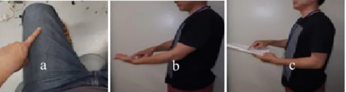
generated by the user's finger tracing a shape onto a bare skinned or covered area on the body. This method inherently filters out errors such as two surfaces overlapping but not touching scenarios which traditional visual methods suffer from. The energy efficient small form factor microphones which were commercially available incorporated into the system allowing for high mobility, captured the resultant TES which was subsequently localized upon using time-difference-of-arrival (TDOA). This localization property allowed for a wide range of inputs as any shape or gestures could be drawn freely on a surface. Existing systems utilize transducers for feedback which are bulky and energy inefficient while this system leverages upon the existing rich sensory system (mechanoreceptors) present within the human skin and proprioception. Tracing of the bare finger done on the bare palm is the best, due to the high density of mechanoreceptors sensitive to vibrotactile stimulus present on the human palm and finger [5][6]. Nevertheless tracing can also be done on parts of the body covered with clothing which can still generate triboacoustic localizable signals and at the same time can be felt by the user as depicted in Figure 1. In the worst case scenario, the tracing can be done on any rough surface present around the user, but with the loss of the rich natural sensory feedback of the human skin. Examples are shown in Figure 1.
Figure 1: Writing with (a) (b)and without (c) natural sensor feedback
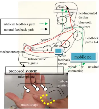
Besides working as a standalone input device, this proposed system could also be merged with other devices such as smart phones or head mounted display which enhances its functionality. The microphone arrays could be connected to the headmounted display and earpiece via the smartphone and worn on the wrist to detect shapes or gestures traced by the finger on the opposing palm. The additional feedback is then relayed back to the user acoustically and/or visually. This idea is depicted in Figure 2.
Additionally, this idea can also be implemented with tactile feedback devices strapped to various parts of the body for individuals who are visually and hearing impaired, as they rely very heavily on their tactile senses to interact with their environment. This thesis evaluated the feasibility of localizing upon TES by first discussing the localizing equations, TES characteristics, realizing all the ideas through the design considerations section and finally verifying the functionality of the developed system by
2 benchmarking it against the visual localization system.
Figure 2: Acoustic input system assimilation
A. Sound Localization Concept
By using cross-correlation, the TDOA between sensors can be attained, for use either with the hyperbolic localization equations or angle of arrival (AOA) method. Figure 3 illustrates the method the problem is viewed in hyperbolic localization method, which is then used to derive the subsequent equations.
Figure 3: Hyperbolic localization method
represents the distance of separation between the sound source and the nth sensor. and represents the
coordinates of the nth sensor.
Both AOA and hyperbolic localization method rely heavily on TDOA for its localization ability. The time difference of arrival TDOA is needed as sound emission times of TES are unknown or uncontrolled. TDOA is attained using (2) [10].
t n,d tdoa = tn -td =
n ≠d (2)
d in (2) also represents the sensors, the reason that n is not equal d is so that all the possible combinations of TDOA can be attained. Variables tn and td represents the
absolute time taken for sound to travel from the sound
source to the sensors, represents the speed of sound. The number of sensors define the number of equations which can be derived from (2) which in turn dictates whether the set of equations are undetermined or overdetermined. Assuming the number of sensors are more than the unknown variables, the system reduces to an elegant overdetermined system. As elegant as the equation might seem, an analytical solution is highly unattainable due to the fact that the TDOA measured is imperfect. This is solved by implementing the said equations numerically via the gradient descent method to get the approximate solutions. xi+1 s = xi s - α F(xi s, yi s) yi+1 s = yi s - α F(xi s, yi s) (3) The velocity of sound is a constant within the equation, as this velocity is the speed of sound within the assumed homogenous properties of air shared by the three sensors. α is the step size for each correction of (xi s, yi s).
The output of the error function F(xi
s, yi s)is evaluated at
each iteration, utilizing the guessed values of coordinates xi s and yi s. If this error value is higher than a user defined
value, the system will try to guess the next improved coordinates’ xi+1
s and yi+1 s values by using the gradient
of the function F(xis,yi s). This process will continue until
the error value set by the user has been achieved or when the number of maximum iterations set by the user has been reached.
Another method of localization using TDOA is AOA. TDOA attained in (2) is used to calculate the angle of which the sound source arrived from in reference to an arbitrary sensor center. With the TDOA from (2), the AOA can be found with the help of (4).
(4)
describes the calculated angle of arrival of the sound source with reference to the axis perpendicular with the base plane, is the distance between the two sensors. Using a minimum of three sensors of known location, localization of a sound source point in two dimensional space via the intersection of the angles of arrivals is attainable as illustrated in Figure 4. Equation (4) has inherent localization accuracy errors as it is an approximation equation. Despite using ideal TDOA values, (4) produced an angle of arrival smaller than that of the actual angle of arrival. As a result, the intersection of the two angle's vector will occur sooner and closer to the base planes as opposed to the actual sound source location. This is illustrated in Figure 4.
Figure 4: AOA illustration
(1) Sensor Sensor Actual Sound source Base plane Ld Sensor ϕ 1, ϕ 2 : angle of arrival Intersection of AOA β1, β2:actual angle of arrival
ϕ2 ϕ1 β1 β2 Sensor A Sensor B Sound source Base plane Sensor C R1 R2 R3 (x1,y1) (x2,y2) (x3,y3) (xs,ys) mobile pc proposed system mechanoreceptors nerve brain headmounted display bluetooth earpiece Feedback paths 1-4 1 2 3 triboacoustic signals nerve 4 wired or unwired connection tactile feedback device artificial feedback path
natural feedback path
traced shape
Triboacoustically emitted signals
microphone s
3 B. Sound of Interest - Scratch Sound
Characteristics
TES is defined as the acoustic signals generated by means of tribology. Acoustic signals are defined as longitudinal waves due to their mode of propagation. Acoustic wave propagation requires medium of transmission. Consequently, the state of the medium which it travels through effects the propagation speed. The approximate speed of sound in dry air (RH = 0%) at 20℃ is 343 ms-1.
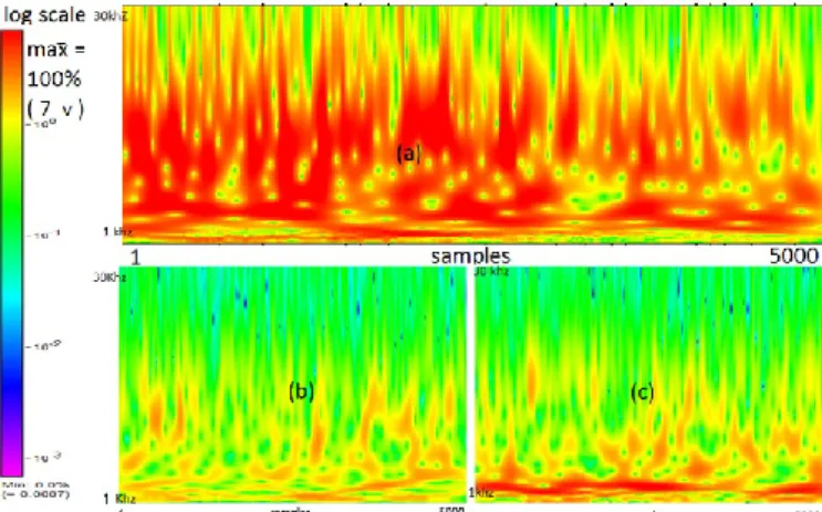
Tribology is a complex science which involves the interaction between two or more surfaces with a net motion larger than zero. In this case, we are interested in the excess energy in the form of sound produced by this interaction at the interface zone for localization purposes [11]. Researchers [11][12] show that tribological interactions between surfaces rigid and elastic alike do generate sound. Acoustic magnitude and frequencies measured by the researchers appear to be white noise dependant on parameters such as materials, surface roughness, roughness wavelength, contact force, surface conditions (oil, Rh% etc) [11], [13].General characteristics discovered by researchers [12] show that the signals generated triboacoustically are quasi-periodic and non-stationary implying that these signals in time domain attained within a specified time frame are unique from the signals collected in the other time frames [12]. Cursory inspection of Figure 5 yields the observation that naturally occurring acoustical signals are neither strictly periodical nor stationary.
Figure 5: Spectrogram (a) scratch sound+ background sound, (b) background noise, (c) voice + background noise
3. DESIGN CONSIDERATIONS
The choices of workspace materials which interacts with the finger of the author is important for this experiment as it defines the values of mutual TES generated. This therefore implies the parameters that effect the finger's vibrational outputs would also most likely effect the acoustic frequency and magnitude. The tribological process in this thesis requires two surfaces to be in contact, human finger (bare or covered) and a generic workplane surface. The generic workplane in this particular thesis was represented by the glabrous skin (palm), cloth and thesis (book). These surfaces were chosen as palm and cloth represented locations which the user can trace a shape on their body with a finger while thesis (book) represents the generic surfaces the user can acquire to trace on if the latter surfaces are unavailable. Skin rheology varies greatly among individuals which are also affected by environmental conditions, hence producing varying magnitudes and frequency of acoustic signals. TES is
known to be white noise, where multiple frequencies exists. By studying the sensor frequency response, 25KHz was chosen as the sensors accentuated this frequency. It incidentally was a high frequency component.
Despite the advantages attained from using higher frequency as the fundamental frequency, literature dictates that the distance of sensor separation for single frequency sound as λ/2 [10][14], which greatly reduces the angle (Φ) resolution as well as increasing the challenge of fabrication of microphone distance separation with the assumption that the sampling rate and bit resolution remain constant. The reduced angle resolution can be explained using (4), by reducing Ld, the finest available unit tn,d tdoa
will represent a larger steps of angle ϕ. Popular solutions would be increasing the sampling rate which would increase the cost or extrapolation which would increase the processing time with non-guaranteed results.
As a solution, it was proposed to utilize the microphone pair distance of separation of the 8th subharmonic of the
assumed fundamental frequency. This solution retains the accuracy advantages from using an assumed fundamental frequency and at the same time addresses the low angular resolution deficiency. Additionally, the increase in sensor separation reduces the complexity of fabrication. This can be described with the postulated fundamental frequency of 25 KHz at the assumed speed of sound of 340ms-1, resulting
in the distance of sensor separation based on [10], as 0.0068m. If the 8th subharmonic of 25 KHz is used with the
same assumptions as above, the distance of separation would be 0.0544m. Referring to (4), it is evident that by increasing the sensor pair distance of separation, the TDOA resolution would increase which in turn would increase the angular resolution Ld, hence increasing the localization
accuracy and resolution without requiring any increase to the sampling rate of the DAQ or extrapolation of measured data. This system therefore had a sensor separation designed for a signal of 3.125kHz but instead measured the TDOA of all detected frequencies.
It was discovered that the utilization of AOA effected the accuracy of the system when the sensors were arranged differently at the already defined distance from one another. Of the three arrangements know, the L-shape provided the best accuracy when evaluated by simulations.
Hardware being imperfect introduced errors to the TDOA measurements. This caused the intersecting lines as in Figure 4 to become intersecting cones instead which yielded multiple coordinates instead of one coordinate.
A. Detection -Triboacoustical Emitted Signals (D-TES)
This system was designed to only respond to scratch sounds. Voice in this particular system is considered as a noise source which occupies the lower frequency bands as shown in Figure 5. Comparing spectrograms in Figure 5 it is easy to discern voice as its energy is mostly contained below the 7kHz band. Incidentally the signal of interest, the scratch sound has similar characteristics with that of voice + background noise where energy is spread across the whole detectable frequency band including below the 7khz level. The slight difference is that voice + background noise has higher ratio of energy in its lower frequency as compared to scratch sound which has higher concentration of energy in the higher frequency bands.
Hence using a simple highpass filter cannot correctly determine whether the sound accepted is that of a scratch sound or some environmental noise .Using FFT we
4 calculate the Decibel ratio of the sum of high frequency vs the sum of the low frequency as shown in (5).
(5)
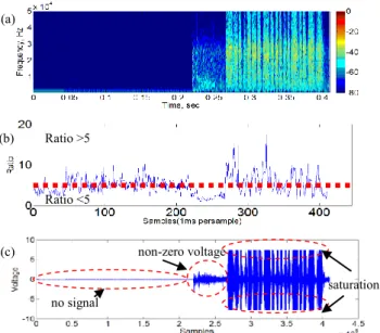
is the ratio of sums between the high and low frequencies components. describes the magnitude of the frequencies attained, while represents the lower limit of the high frequencies and represents the upper limit of high frequencies. In this case, it was set to 8KHz and 30KHz. represents the lower limit of low frequencies and reprsents the upper limit of low frequencies which was defined as 1KHz and 7KHz. The accepted ratio of this system was above 5.
Despite the best of efforts to keep the resultant noise low, noise will still be picked up by the system, hence a simple voltage thresholding method is used to counter this noise floor. Besides setting the noise floor threshold, a maximum limit voltage setting was also set, to avoid saturation signals from being accepted for evaluation. Saturated signals have flat peaks which basically produces very poor TDOA. This happens as the generation of TES is difficult to control, hence many factors can drive the amplifiers into saturation. Saturation limit was set to 97% of the actual saturation value. The implemented method is shown in Figure 6.
Figure 6: D-TES (a) Spectrogram (b) ratio of frequency magnitude (c) signal magnitude before D-TES Hence the D-TES is a combination of the voltage range and frequency ratio method, any signal which qualifies is then allowed to proceed to the next level of processing which is the cross-correlation process to find the TDOA. Various methods have been proposed for attaining TDOA, but the most basic idea is to discern the time difference between two signals caught by two spatially displaced sensors. Methods to do so range from the time domain to the frequency domain. In this particular thesis, cross-correlation in the time domain was used as it was the simplest method to implement.
(6)
Cross-correlation is described in (6) where stands for
the signal in the first sensor, stands for the signal arriving in the second sensor, stands for the discrete time,
stands for the discrete time epoch, stands for the product sum of the two signals. When is the
maximum value, it implies that the two signals are at the best match at the corresponding time epoch. At this point, the TDOA between the two sensors is defined as . The sound source can be localized upon by incorporating the TDOA into the AOA methodology explained in the previous section.
B. Test-bed Setup
The basic idea of this thesis is to test the viability of using scratch sound as a computer input medium. The abilities and constraints as mentioned in the introduction are to be tested with some simple tests. The most important feature is its ability to decipher and localize upon TES generated by tracing a finger (bare or covered) on human skin and on some random surface. Experimental hardware setup as in Figure 7 was configured based upon the evaluations done in the previous sections.
Figure 7: Hardware setup
The TES generated from the interactions of the finger with the active material in the workspace were caught by three spatially displaced microphones (SPM040LE5H) which were subsequently converted into electrical signals to be fed to the amplifier. It was taken into account that such acoustical signals were extremely small and therefore required large amplification. In this particular set up the authors used a 2.5k, two stage amplification to amplify the signals from the microphones which have already been pre-amplified within its SMD body. These pre-amplified analog signals were then channeled to a 12 bit DAQ sampling at the rate of 1MSa/s which were then converted into digital data and processed by the algorithms written in the computer for localization. Derived localized points are then displayed and stored on the computer in real time. Simultaneously, when the finger was being traced upon a surface, a camera was used take video at 300 frames per second with graph thesis in its field of view (FOV) for accuracy verification and scaling as shown in Figure 8.
Light Monitor C P U D A Q high speed camera acoustic sensors workplane saturation no signal non-zero voltage Ratio >5 Ratio <5 (a) (b) (c)
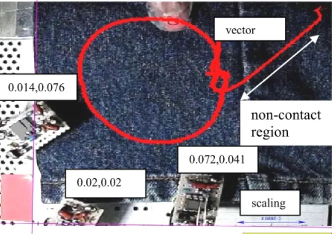
5 Figure 8: Visual tracking post-processing
In this particular case in Figure 8, the surface used was made from denim material. The finger was marked with red and black to assist the software to better discriminate it from the background. Purple lines on the left and bottom mark the declaration of the y-axis and x-axis. The cumulative arrows marked the passage of the finger at every frame detected by the software. The actual motion during contact with the cloth/work surface was a circle, while the additional lines were caused by the entry and exit of the finger into and from the FOV during non-contact times. This data was then used as the benchmark for comparison against data attained from the acoustic based localization. The surfaces prepared were, human palm (glaborous skin), cloth and book surface. As for the finger conditions, tests were done bare skinned or with covers (plastic or thesis covers) as shown in Figure 9.
Figure 9: (a) Bare Finger (b) thesis covered finger (c) plastic covered finger
The author's finger was washed with hand soap. It was then dried with tissues and subsequently left to be air dried in the experimentation room with humidity and temperature of RH60% and 25.6℃ for five minutes prior to experimentation. Some results are shown as in Figure 10.
Figure 10: Results (a) bare finger scratch palm (b) plastic covered finger scratch palm
The dotted lines in Figure 9 represent the visually attained data while the solid line represents the acoustically produced line. It can be seen that the acoustic method is able to re-created the shape but not the size. This method was inherently impervious to the no-contact times of the finger with the surface unlike the visual system. This was shown as in Figure 8 and Figure 9. This section managed to prove the possibility of using TES generated from the
action of the finger tracing onto any surface. This size change was most likely due to the sensor offsets which would be studied in detail in the next section.
4 IMPROVEMENTS 1
This section addresses the problem seen in the first prototype where the shapes created were smaller. The problem was simulated and the parameters which showed to be affected in the simulations were improved in real life and verified.
It was discovered through simulations and actual experiments that the shrinking shape problem faced in the first prototype was caused by the offset in the z-axis between the workplane plane and sensor plane.[15]
Figure 11: (a) sensor plane offset in z axis by +0.03m simulations (b) sensor plane offset in z axis by +0.03m
experiments
In addition to that, it was also discovered that any displacement of a sensor in the x or y axis causes not only size changes, but also shape changes of the shapes re-created.
Figure 12:(a)sensor offset by 0.005 simulations (b)sensor2 offset in x axis by +0.01m
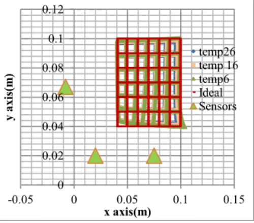
Temperature of air in which the acoustic signal travels through affects the speed of sound. It was shown through simulations that by using the AOA algorithm, the offset of up to 26° C does not affect the localization much and in fact is some cases improved upon the AOA algorithm's weaknesses. This is shown in Figure 13.
0.0 0.1 0.2 0.0 0.1 0.2 y axi s(m ) x axis(m) 0.0 0.1 0.2 0.0 0.1 0.2 y axi s( m ) x axis(m) 0 0.05 0.1 -0.02 0.03 0.08 y ax is( m ) x axis(m) Ideal AOA Disp 0.03m Sensors 0 0.05 0.1 -0.02 0.03 0.08 0.13 y ax is( m ) x axis(m) AOA z shifted 0.03m visual 0 0.05 0.1 -0.02 0.03 0.08 y ax is( m ) x axis(m) s2 x+0.005 Ideal Sensors 0 0.05 0.1 0.15 -0.02 0.03 0.08 0.13 0.18 y ax is( m ) x axis(m) sensor 2 offset 0.01m x axis visual vector scaling 0.014,0.076 0.02,0.02 0.072,0.041 (a) (b) non-contact region non-contact region (a) (b) (a) (b)
6 Figure 13: Temperature mismatch
Physical experiments were not conducted for temperature mismatch as the simulations showed very little effect to the accuracy of the system. This implied that any errors introduced by the incorrect usage of temperature could hide the errors introduced by the AOA algorithm. 5. IMPROVEMENTS 2
Because of known errors of the AOA, the author focused on creating and validating new algorithms which could be accurate like the GDM of hyperbolic equations but at the same time be as fast as AOA. Main issues which plague GDM were the initial starting position which causes issues in convergence. This can be further exacerbated if the error function was crafted to have many local minima. Normal methods in solving such issues are to craft a very good error function with global minima located at the end of a steep gradient and with none or few local minima. Another common method is to create new algorithms which can traverse across any error function to reach the global minima fast and without problems.
This innovative method used the AOA to set the initial starting position for the GDM. The AOA placed the initial starting position of the GDM close to the final answer hence allowing to avoid the local minima issues altogether. This is shown in Figure 14.
This was implemented through simulations of such equations in a imaginary workplane using pseudo-coordinates where 2-D error maps or 3-D error mesh plots are created for each coordinate point with the best solution which yielded the lowest error is then tested in real-time and further improved upon based on detected shortcomings. The hyperbolic method when used without the speed of sound Vs as in (7) with three acoustic sensors yielded an
3-D error mesh plot which was a trench implying multiple convergent points, which was an inconclusive localization coordinate. |[((x1 - xs)2 + (y1- ys)2)1/2 -(( x2- xs)2 + (y2- ys)2)1/2] . t13 - [((x1 - xs)2 + (y1- ys)2)1/2 -(( x3 - xs)2 + (y3- ys)2)1/2] . t12 | +|[(( x1 - xs)2 + (y1- ys)2)1/2 -(( x2 - xs)2 + (y2- ys)2)1/2] . t23 - [((x2 - xs)2 + (y2- ys)2)1/2 -(( x3 - xs)2 + (y3- ys)2)1/2] . t12 | + |[(( x1 - xs)2 + (y1- ys)2)1/2 -(( x3 - xs)2 + (y3 -ys)2)1/2] . t23 - [((x2 - xsv + (y2- ys)2)1/2 -(( x3 - xs)2 + (y3 -ys)2)1/2] . t13 |=0 (7)
The usage of four acoustic sensors yielded an 3-D error mesh plot of inverse cone. This implied a single convergent point which was good. But utilized an extra sensor which
would reduce the device's mobility. The equation was then reverted back to (8) which was dependent upon the speed of sound which in turn was dependent upon the temperature of air. |(t12 . Vs ) - [((x1 - xs)2 + (y1- ys)2)1/2 -(( x2 - xs)2 + (y2 -ys) 2)1/2]| + |( t13 . Vs) - [((x1 - xs)2 + (y1- ys) 2)1/2 -(( x3 - xs)2 + (y3- ys)2)1/2 ]| + |( t23 . Vs) -[(( x2 - xs)2 + (y2 -ys)2)1/2 - ((x3 - xs)2 + (y3- ys) 2)1/2]| =0 (8)
Figure 14:3D Error mesh plot of one set of TDOA
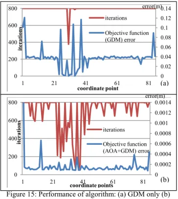
Results from simulations indicate that the temperature difference did affect the localization accuracy. This equation was then modified to function in an iterative method where it self-corrects errors introduced to the pseudo coordinates. GDM and was found to be able to self correct to an average minimization error of 0.000097m, despite that, the iterations which is the time taken to do so was very long, an average of 1256 iterations per coordinate.
An innovative method of merging the AOA with GDM resulted in a faster and more accurate localization algorithm which was simulated and tested in real-life. In simulations, it achieved an average of 373 iterations as compared to using full GDM which required 1256 iterations.
0 0.02 0.04 0.06 0.08 0.1 0.12 -0.05 0 0.05 0.1 0.15 y ax is( m ) x axis(m) temp26 temp 16 temp6 Ideal Sensors . correct coordinate randomly, first guessed coordinates (far from correct coordinate)
AOA calculated coordinates (near to correct coordinate)
7 Figure 15: Performance of algorithm: (a) GDM only (b)
AOA and GDM
Real-life experiments yielded an average iteration of 363 iterations per coordinate. This method which focused on finding the convergant point with the smallest iteration number could be utilized in many other 2-D localization applications which require higher speeds of attaining the results. The result of the experiment is as shown in Figure 16.
Figure 16: Real-life experiment on dorsal of hand This method successfully introduced a new approach to solving GDM convergent issues in a simple and effective method. Tests so far were conducted in laboratory environment which has its background noise controlled. For his device to be truly versatile, it had to be designed to be robust in all acoustic environments.
6 IMPROVERMENT 3
The device was to be used in various locations an algorithm which separates it from background noise needed to be created to make it robust. A spatial method was used to create groups to segregate the arriving acoustic coordinates cn based on their velocity between one another
based on the concept that it is not likely that the user's finger moved very quickly across the surface of the workplane. This concept is illustrated in Figure 18.
Figure 17: Coordinate arrivals
Figure 18: Self-learning, self-segregating algorithm concept Once the groups were defined, the segregation of subsequent arriving coordinates were defined by the Cartesian distance of the coordinate to the mean Ma/b of the
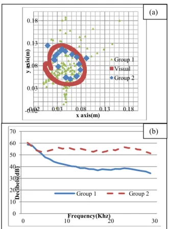
groups previously created. Every new member added to a group updates the group's mean therefore giving this method a real-time learning capability which makes it versatile. This, together with an innovative usage of LED's to synchronize the data collected acoustically and visually was able to verify the effectiveness of the proposed algorithm under lab conditions where the noise was produced by earphones. Some of the results are as in Figure 19. It was found that the system not only could segregate the TES from simulated noises, but could also pin-point the location of the noise as long as it had similarities to white noise characteristics.
Figure 19: (a) voice interference (b) white noise interference 0 0.05 0.1 0.15 0.2 0 0.05 0.1 0.15 0.2 y a xi s (m ) x axis(m) Corrected AOA acoustic Acoustic AOA visual(Ideal) Mb c1 c2 c3 Ma v12 v23 v13 db3 da3 x axis y axis group A group B c = coordinates of detected sound sources v = velocity M= center of group d = distance -0.02 0.03 0.08 0.13 0.18 -0.02 0.03 0.08 0.13 0.18 y ax is( m ) x axis(m) Group 1 Group 2 Group 3 Speaker Microphones Visual -0.02 0.03 0.08 0.13 0.18 -0.02 0.03 0.08 0.13 0.18 y ax is( m ) x axis(m) Group 1 Group 2 Group 3 Speaker Microphones Visual 0 0.02 0.04 0.06 0.08 0.1 0.12 0.14 0 200 400 600 800 1 21 41 61 81 it er at io ns coordinate point iterations Objective function (GDM) error 0 0.0002 0.0004 0.0006 0.0008 0.001 0.0012 0.0014 0 200 400 600 800 1 21 41 61 81 it er at io ns coordinate points iterations Objective function (AOA+GDM) error (b) (a) error(m) error(m) (a) (b)
8 Automatic segregation was successful. A more advanced method should be created to segregate the coordinates not only by spatial means but by frequencies as well.
7. IMPROVERMENT 4
The method previously proposed was further refined where the Group creation concept was maintained but the segregation of the groups was modified. Instead of only relying on spatial distances, the Euclidean distances of acoustic frequencies from 1-29KHz in 1KHz increments from the detected and localized acoustic sources were used instead. The Euclidean vector is defined as . while
stands for the parameters. This is shown as in (9)
(9)
The Euclidean distance is defined as as shown in (10).
=
(10)
This therefore allowed for the system to learn the frequency characteristics of its ever changing environment and TES. This allowed it to use both spatial and frequency components to segregate the. This algorithm was tested in a miniaturized hardware on various surfaces in real-life noisy environments which yielded relatively good results. Samples of results are as in Figure 20(a) for TES which generally have a magnitudes larger in all frequencies than the background noise Figure 20(b).
Despite the success, there were some experiments where the sensors were driven to saturation by the background noises failed to localize and segregate properly.
This prompted the usage of acoustic barriers on the microphones which could block background noises from saturating the microphones and at the same time amplify the arriving TES as shown in Figure 21.
Figure 20: results, cloth in hallway (a) localization (b) frequency characteristics
This barriers served two purposes, first to reflect unwanted noise and second to amplify the TES. The measurement of the barrier ensured that the high frequency components were reflected away and amplified. as can be seen in Figure 22 (b).
Figure 21: acoustic barriers, side view
The results show that despite being able to do as designed, the re-created shapes although retaining their shapes were of smaller sizes. This is shown in Figure 22.
Figure 22: Mitigation results, table surface with finger (a) localization (b) frequency characteristics More work has to be done in this area of acoustic barriers.
8. CONCLUSION
This thesis introduced a new method of mobile device input which maintains the mobility of the device, via its usability on multiple surface available in the environment, lightweight, and low power consumption. It at the same time affords users a large range of inputs and ease of use
0 10 20 30 40 50 60 70 0 10 20 30 D ec ib el s( dB ) Frequency(Khz) Group 1 Group 2 (b) -0.02 0.03 0.08 0.13 0.18 -0.02 0.03 0.08 0.13 0.18 y ax is( m ) x axis(m) Group 2 Visual Group 1 0 10 20 30 40 50 60 70 0 10 20 30 D ec ib el s( dB ) Frequency(Khz) Group 1 Group 2 (b) (a) High frequency signals (noise) side view (a)
TES ray direction
Workplane surface finger -0.02 0.03 0.08 0.13 0.18 -0.02 0.03 0.08 0.13 0.18 y ax is( m ) x axis(m) Group 1 Visual Group 2 (a)
9 through the detection and localization of TES from the action of users tracing on various surfaces.
REFERENCES
[1] M. Ahmad, The Next Web of 50 Billion Devices: Mobile Internet’s Past, Present and Future
(Smartphone Chronicle). North Charleston:
CreateSpace Independent Publishing Platform, 2014.
[2] B. Sanou, “2014 ICT Facts and Figures,” International Communication Union 2014.
[3] C. Harrison and A. D. Wilson, “OmniTouch : Wearable Multit ouch Interaction Everywhere,” in Proceedings of the 24th annual ACM symposium on
User interface software and technology - UIST ’11,
2011, pp. 441–450.
[4] C. Harrison, D. Tan, and D. Morris, “Skinput : Appropriating the Body as an Input Surface,” in 28th Annual SIGCHI Conference on Human
Factors in Computing Systems, 2010, pp. 453–462.
[5] T. Deyle, S. Palinko, E. S. Poole, and T. Starner, “Hambone: A Bio-Acoustic Gesture Interface,” in 2007 11th IEEE International Symposium on
Wearable Computers, 2007, pp. 3–10.
[6] H. Sasaki, T. Kuroda, P. Antoniac, Y. Manabe, and K. Chihara, “HAND-MENU SYSTEM : A DEVICELESS VIRTUAL INPUT INTERFACE FOR WEARABLE COMPUTERS,” J. Control
Eng. Appl. Informatics, vol. 8, no. 2, pp. 44–53,
2006.
[7] H.-S. Yoon, J. Soh, Y. J. Bae, and H. Seung Yang, “Hand gesture recognition using combined features of location, angle and velocity,” Pattern Recognit., vol. 34, no. 7, pp. 1491–1501, Jan. 2001.
[8] A. Rogowski, “Industrially oriented voice control system,” Robot. Comput. Integr. Manuf., vol. 28, pp. 303–315, 2012.
[9] X. Han, H. Seki, Y. Kamiya, and M. Hikizu, “Wearable handwriting input device using magnetic field,” Precis. Eng., vol. 33, no. 1, pp. 37–43, Jan. 2009.
[10] K. C. HO and Y. T. Chan, “Solution and performance analaysis of geolocation by TDOA,”
Aerosp. Electron. Syst., vol. 29, no. 4, pp. 1311–
1322, 1993.
[11] H. Zahouani, R. Vargiolu, G. Boyer, C. Pailler-Mattei, L. Laquièze, and a. Mavon, “Friction noise of human skin in vivo,” Wear, vol. 267, no. 5–8, pp. 1274–1280, Jun. 2009.
[12] K. Asamene and M. Sundaresan, “Analysis of experimentally generated friction related acoustic
emission signals,” Wear, vol. 296, no. 1–2, pp. 607–618, 2012.
[13] H. Zahouani, S. Mezghani, R. Vargiolu, T. Hoc, and M. El Mansori, “Effect of roughness on vibration of human finger during a friction test,” Wear, vol. 301, pp. 343–352, 2013.
[14] I. J. Tashev, Sound Capture and Processing:
Practical Approaches. Wiley, 2009.
[15] Y. W. Leong, H. Seki, Y. Kamiya, and M. Hikizu, “TRIBOACOUSTIC LOCALIZATION SYSTEM FOR MOBILE DEVICE - ENVIRONMENTAL EFFECTS TO ACCURACY,” Int. J. Smart Sens.