(will be inserted by the editor)
Pairwise Meta-Rules for Better Meta-Learning-Based
Algorithm Ranking
Quan Sun · Bernhard Pfahringer
Received: 20 January 2013 / Accepted: 24 May 2013, DOI: 10.1007/s10994-013-5387-y
Abstract In this paper, we present a novel meta-feature generation method in the context of meta-learning, which is based on rules that compare the performance of individual base learners in a one-against-one manner. In addition to these new meta-features, we also introduce a new meta-learner called Approximate Ranking Tree Forests (ART Forests) that performs very competitively when compared with several state-of-the-art meta-learners. Our experimental results are based on a large collec-tion of datasets and show that the proposed new techniques can improve the overall performance of meta-learning for algorithm ranking significantly. A key point in our approach is that each performance figure of any base learner for any specific dataset is generated by optimising the parameters of the base learner separately for each dataset.
Keywords Meta-learning·Algorithm ranking·Ranking trees·Ensemble learning
1 Introduction
Training a good model for a given dataset is one of the common tasks of a data analyst. The straightforward approach of simply applying and optimising all known learning algorithms is usually not feasible. Thus an experienced data analyst will gen-erally perform some form of preliminary analysis and then focus on a few promising algorithms. This selection is guided by the prior experience of the analyst. Meta-learning tries to support and automate this process. It tries to predict the probably best or close to best algorithms, thus considerably reducing the amount of training and optimisation time needed for finding a good model on a given dataset. This re-duction in resource consumption should be accompanied by no or only a small loss in predictive performance when compared to the best possible result [8, 7]. Meta-learning for algorithm ranking uses a general machine Meta-learning approach to generate Quan Sun·Bernhard Pfahringer
Department of Computer Science, The University of Waikato, Hamilton, New Zealand E-mail: qs12,[email protected]
meta-knowledge mapping the characteristics of a dataset, captured by meta-features, to the relative performances of the available algorithms.
The advantage of the meta-learning approach is that high quality algorithm rank-ing can be done on the fly, i.e., in seconds, which is particularly important for busi-ness domains that require rapid deployment of analytical techniques. In machine learning research, meta-learning has also been used for boosting the performance of evolutionary-algorithm-based model selection techniques [33]. The work by [36] has discussed cross-disciplinary perspectives on meta-learning. Theoretical motiva-tions on meta-learning research are due to the No Free Lunch (NFL) theorem [42] and the Law of Conservation for Generalization Performance (LCG) [34]. Recent re-search seems to suggest that it is possible to show that meta-learning offers a viable mechanism for building a “general-purpose” learning algorithm [17]. For a compre-hensive review of meta-learning research and its applications, we refer the reader to [17, 7, 21, 35].
This paper makes three contributions: a novel feature generator for meta-learning, a new meta-learner, and a more appropriate experimental configuration, for improving the overall performance of meta-learning for algorithm ranking.
2 Background
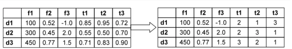
“Meta-learning” is a broad field; in this paper, for simplicity, the term meta-learning is used in the sense of “meta-learning for algorithm ranking or recommendation”. We first introduce the mechanics of meta-learning. The basic steps of a meta-learning task are as follows. Firstly, a set of datasets is collected; secondly, we need to define some meta-features as the characteristics of each dataset, e.g., the number of instances, the number of numeric or categorical features, and many more; for more details on meta-features please refer to Section 3. Thirdly, we estimate the predictive performance of the available algorithms, e.g., using cross-validation, for every dataset in the dataset collection. Thus, for each dataset we get a list of available algorithms with their per-formance estimates. Given the above information, we can construct a meta-dataset, which is an×mdata matrix, wherem=mf+mt. Here,mis the sum of the number of meta-featuresmf and the number of algorithmsmt, andnis the number of datasets. Figure 1 (left-hand side table) shows an example of a meta-dataset in a general multi-target regression setting.
For algorithm recommendation, our goal is not to predict the absolute expected performance of any algorithm, but rather the relative performance between algo-rithms. Thus, the meta-dataset can be transformed to represent the rankings of the algorithms. Figure 1 (from left-hand side to right-hand side table) shows an example of how a “raw” meta-dataset is transformed. In this case, ranking is a special case of the general multi-target regression setting. Then, a meta-learner, which we will call it a “ranker” here, will take thisn×mmatrix as its training input to learn a ranking model. Given a new dataset, we first calculate its features and use the meta-features (e.g., the f1,f2,f3values for the example in Figure 1) as input to the ranker. The ranker finally returns a ranked list of all algorithms. As is true in general for ma-chine learning, the performance of meta-learning depends crucially on the quality of
Fig. 1 Two formats of a meta-dataset constructed from three datasets (d1,d2,d3), three meta-features
(f1,f2,f3) and three algorithms (t1,t2,t3). Left-hand side table shows the format using the actual
perfor-mance values (higher is better) as targets; the right-hand side table shows a format using the ranks (lower is better) as targets.
both the meta-features and the meta-learners available. In addition, the performance of the base-level learners must also be estimated to a high quality to enable successful meta-learning.
Existing meta-learning systems are mainly based on three types of meta-features: statistical, information-theoretic and landmarking-based meta-features, or SIL for short. Thorough reviews of these meta-features can be found in [6, 31, 23, 37]. Re-cently, more meta-feature sets have been developed, for example, the learning-curve-based meta-features [26], tree-structure-information-learning-curve-based [3] and histogram-learning-curve-based [23].
In this paper, we propose a novel method for meta-learning that generates “meta-level” meta-features from the “base-“meta-level” meta-features via rule induction that tries to predict the better algorithm for each pair of algorithms. Here the “base-level” meta-features can come from any of the meta-feature sets mentioned above. Meta-meta-features generated by the proposed method (described in Section 3) contain pairwise infor-mation between algorithms. Adding them to the original feature space can help to improve the performance of many meta-learners.
Next, we will discuss several ranking approaches from analgorithmicperspective as the underlying multi-target or ranking problem is being studied in various fields, including social sciences, economics and mathematical sciences. Although the ter-minologies and presentations of the same models can be quite different for different fields, the algorithmic properties are similar in concept and relatively easy to describe.
2.1 Thek-Nearest Neighbors Approach
Thek-NN ranking approach has two steps: the nearest neighbor search step and the ranking generation step. In the first step, given a new dataset, we first calculate its meta-features to construct an instance as a query (anmf-value array). Then, we select a set of instances (nearest neighbors) in the training set (then×mf data matrix) that are similar to the query instance. The similarity between instances is usually based on a distance function, e.g., Euclidean distance. In the second step, we combine the rankings of the nearest neighbors to generate an aggregated algorithm ranking for the new dataset. For our experiments, we use the average ranks method described in [7]. LetRi,jbe the rank of algorithmTj,j=1, ...,ton dataset i, wheretis the number of algorithms. The average rank for each algorithmTjis defined as: ¯Rj= (∑ki=1Ri,j)/k, wherekis the number of nearest neighbors. Thek-NN ranker’s performance is related to the value ofk, appropriate values forkare usually determined by cross-validation.
Thek-NN ranker is often used as a benchmark learner for testing the performance of different meta-feature sets.
2.2 The Binary Pairwise Classification Approach
Given then×mdata matrix as the training data, multiple binary (pairwise) classifi-cation models can be used to construct a ranking model. For example, if there were three meta-features and three algorithms in the training set (e.g., Figure 1 right-hand side table), one could build three binary classification models for each pair of algo-rithms: Algorithm-1 vs. Algorithm-2, Algorithm-1 vs. Algorithm-3, and Algorithm-2 vs. Algorithm-3. The training data for the three binary classification models are the same, which is the n×mf data matrix. Given a new dataset, we first calculate its meta-features, again anmf-value array as a query. Then, we use the three binary clas-sification models to classify the query. The final algorithm ranking list for the new dataset is computed based on how many times each algorithm has been predicted as “is better”. If there were more than three algorithms to rank, then there might be ties in the list. Several tie breaking techniques have been examined in the literature [23, 7], but usually this choice does not have a strong influence on the performance of a meta-learning system.
The advantage of the binary classification ranking approach is that existing binary classification algorithms can be employed directly. However, if there are many algo-rithms to rank, then the number of binary models required can be large and hard to manage in practice, e.g., for 20 algorithms, this would requireT×(T2−1)=20×219=190 binary classification models to be built, which could be costly if one also considered using different – and fine tuned – classification algorithms for each of the 190 binary classification problems. The binary pairwise classification approach has also been studied in label ranking [20].
2.3 The Learning to Rank Approach
From the end-user’s perspective, algorithm ranking is similar to the ranking problem in a search engine scenario, where a ranked list is returned for responding to a query. The search engine scenario has been extensively studied in learning to rank and in-formation retrieval (IR). One obvious candidate for rank prediction is the AdaRank algorithm proposed in [43]. AdaRank is a boosting algorithm that minimizes a loss function directly defined on the ranking performance measure. The algorithm repeat-edly constructs “weak rankers” on the basis of re-weighted training data and finally linearly combines the weak rankers for making ranking predictions. In addition to supplying algorithms, the IR literature is also an excellent source for ranking evalu-ation metrics. Similar to search engine users, meta-learning users are usually mainly interested in the top candidates, be it websites or algorithms. An IR measure which captures this bias towards the top ranked items well is the normalized discounted cumulative gain (NDCG) metric [22, 29], which has not been used in meta-learning evaluation previously.
2.4 The Label Ranking Approach
Label ranking can be seen as an extension of the conventional setting of classifica-tion. The former can be obtained from the latter by replacing single class labels by complete label rankings [12, 11]. From an algorithmic view point, one type of label ranking approach, such as the ranking by pairwise comparison (RPC) algorithm [20], is based on extending the pairwise binary classification approach by using more so-phisticated ranking aggregation methods. Another type of label ranking algorithm, such as the label ranking trees (LRT) algorithm [11], tries to apply probabilistic mod-els under the label ranking setting. Meta-learning for algorithm ranking using the multi-target regression setting can also be transformed to a label ranking problem, so that label ranking algorithms can be used directly.
2.5 The Multi-Target Regression Approach
As we can see in Figure 1, the algorithm ranking problem can also be seen as a multi-target (multi-response) regression problem, where the rank position values of each algorithm are the targets in the multi-target regression setting. In multi-target regression, the task is to estimate several target, or response variables using a common set of input variables or features. Two approaches are usually employed. One is to build separate single-target regression models for each target variable; the other is to use a single model to estimate all the targets simultaneously. For meta-learning, the former approach is similar to the binary classification ranking approach but requiring fewer models to be built, e.g., for 20 algorithms, only 20 single-target regression models are needed. In this section, we focus on the latter approach and start from the linear model. A linear multi-target regression model can be expressed as:
Y=XW∗+E, (1)
whereW∗is the regression coefficient matrix (ann×mf matrix),Xis the data (fea-ture value) matrix,Yis the target matrix (which can be rankings) andEis the noise term matrix. The problem is usually formulated as a single convex optimisation prob-lem of the form:
minimize
W f(W)subject tog(W)≤r, (2)
wheref(W)is a loss function, e.g., squared loss,g(W)is the regularization term, e.g.,
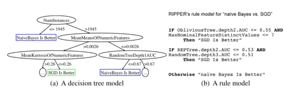
l2-norm-based, andris a constant. Although this kind of formulation is mathemati-cally straightforward, efficient numerical techniques and relatively easy-to-implement algorithms are not readily available for sophisticated ranking-based loss/regularization functions. Also, algorithms in this category are usually designed for relatively low-dimensional problems or it is assumed that the number of training instances is much greater than the number of features, or the number of model parameters to estimate. In addition, we know that the various kinds of meta-features are “logically” related, so a nonlinear model might be more appropriate. Figure 2 shows two model output examples from a decision tree learner and a propositional rule learner for a binary-classification-based meta-learning problem, where only two algorithms are consid-ered. In this example, three types of meta-features (SIL) are used. We can see that
(a) A decision tree model (b) A rule model
Fig. 2 Relationships between base-level meta-features.
whether an algorithm is preferred depends on some logical relationships between meta-features. For example, the second rule in Figure 2 (b) suggests that when there are no strong features (indicated by the “weak” tree-based landmarkers’ AUCs being low) then SGD (a WEKA implementation of an algorithm based on stochastic gradi-ent descgradi-ent) is likely to work better than Naive Bayes. For these reasons we leave the linear, single-model multi-target approach for future research.
Here, we focus on a special class of algorithms that are based on a nonlinear multi-target model:
Y=z(X), (3)
wherezis a decision-tree-based function. A well-known algorithm of this kind is called predictive clustering trees (PCT) [5], which have been adapted for ranking problems in [40]. There are several advantages in using decision-tree-based rankers, including: a decision tree naturally identifies partitions of the data, where “similar” individuals are supposed to be in the same “cluster”. This leads to a relatively natural interpretation for the meta-learning mechanism at the conceptual level; decision tree algorithms are reasonably fast as their training complexity isnlogn, wherenis the number of training instances. In Section 4, we introduce a new ranker, which is an ensemble of decision-tree-based rankers.
3 Pairwise Meta-Rules
In this section, we introduce a novel meta-feature generation method in the context of learning. The main motivation comes from our observation that existing meta-feature sets have ignored one potential source of information: the logical pairwise relationships between each pair of the target algorithms to rank. Explicitly adding this information to the meta-feature space might improve a meta-learner’s predictive accuracy.
Of course, when predicting for a new dataset, this information will not be avail-able, as otherwise we would not try to predict rankings in the first place. Therefore we propose to use a rule learner to learn pairwise rules first, and then use these rules as new meta-features. Two steps are involved: the first step is similar to the binary classification ranking approach, where T×(T2−1) (T is the number of algorithms to rank) binary classification training datasets are constructed from the originaln×m
Fig. 3 Example datasets for learning pairwise meta-rules.
data matrix. Each binary dataset has two class labels:{“algorithmti is better”, “al-gorithmtjis better”}. Whether an algorithm is better than the other is determined by their ranking position in the ranked list of a particular dataset.
Taking the dataset illustrated in the right-hand side table of Figure 1 as an exam-ple, we need to construct 3×(32−1)=3 binary datasets as shown in Figure 3. Then, we build 3 rule-based binary classification models based on the 3 binary classification meta-datasets. In principle any rule learner could be used. We choose the RIPPER algorithm [13], because it is relatively fast and its rule models are generally very compact compared to other rule learners. Figure 2 (b) shows a RIPPER rule model. For each pair of algorithms, we compute a ruleset describing in which situation an al-gorithm is to be preferred over another. We call these rules the Pairwise Meta-Rules. Next, we discuss how these rules can be used as new meta-features. Using Figure 2 (b) as an example, this RIPPER ruleset comprises three rules. The first two are individual rules, whereas the third one is a default catch-all rule. We generate two different sets of meta-features from Pairwise Meta-Rules.
Method 1turns each individual rule into one boolean meta-feature. For example, we may have a Pairwise Meta-Rule:
If BaseMetaFeature-X ≤ 0.5 AND BaseMetaFeature-Y ≥ 0,
Then Algorithm A is better than Algorithm B.
The value of the new meta-feature constructed from this Meta-Rule will be deter-mined by looking at the (base-level) meta-feature values of a new dataset defined by a Meta-Rule. For a new dataset, the Meta-Rule-based meta-feature value is set totrue
if the rule condition “BaseMetaFeature-X ≤ 0.5 AND BaseMetaFeature-Y ≥ 0” is met, otherwisefalse. For the meta-learning problem, the RIPPER algorithm returns on average about two individual rules for each of the 190 algorithm pairs.
Method 2creates just one boolean meta-feature representing the outcome of ap-plying the full ruleset. For a new dataset, the Meta-Rule-based meta-feature value is set totrueif the default catch-all rule of a ruleset is true, otherwise false. For the meta-learning problem, the RIPPER algorithm returns 190 rulesets for each of the 190 algorithm pairs, so in Method 2, 190 Meta-Rule-based meta-features are added to the original feature space.
The Pairwise Meta-Rules method is different from the standard stacking [41] method, where we do not use the predicted complete ranking of base models instead we use the RIPPER rule sets to construct new meta-features. A meta-learner will use all meta-features (including both base-level and Meta-Rule-based meta-features) for building the final model, which is also different from stacking.
In the experiments reported below we compare three different meta-feature sets:
SIL+Meta-Rules-1: the 80 SIL meta-features plus meta-features generated by Method 1;
SIL+Meta-Rules-2: the 80 SIL meta-features plus meta-features generated by Method 2.
Next, we propose a novel meta-learner (ranker), specifically designed for the meta-learning-based algorithm ranking problem.
4 Approximate Ranking Tree Forests for Meta-Learning
In preliminary experiments we found that the predictive performances of the predic-tive clustering trees for ranking (PCTR) [40] and the label ranking trees (LRT) [11] algorithms usually are worse than the optimisedk-NN ranker for our meta-learning problem, where the number of objects to rank is relatively large (20 algorithms). In-spired by the bootstrap aggregating (bagging) [15, 9] strategy and the random forests framework [10], we here propose a new ranker for the meta-learning problem, called Approximate Ranking Tree Forests (ART Forests), which is a random forest ensem-ble of approximate ranking trees. The motivations for proposing ART Forests include: 1. as more and more meta-features are being developed and added to the feature space, we believe that a relatively fast algorithm (e.g., decision-tree-based learn-ers) that has “built-in” feature selection capacity would be useful;
2. the meta-learner should not be constrained by the “number of training examples must be much greater than the number of parameters to estimate” restriction, because for the meta-learning problem the number of datasets is usually not very large;
3. recent theoretical work [4] seems to suggest that irrelevant features do not sig-nificantly decrease random forest’s predictive performance, so ideally the meta-learner should be capable of using as many meta-features as possible;
4. ensemble algorithms usually outperform base algorithms. Statistics and models aggregated from bootstrap samples are nonparametric estimates [15], so we do not have to make parametric assumptions about the form of the underlying pop-ulation, which provides an automatic approximation layer to our new algorithm. In the literature, an empirical study by [24] has shown that boosting-based meta-learner outperformed thek-NN based meta-learner in the pairwise binary classi-fication setting (Section 2.2) for meta-learning.
4.1 Approximate Ranking Trees (ART)
In this section, we propose the ART algorithm which is used as the base learner for ART Forests. The pseudocode is given in Algorithm 1. ART is a recursive partitioning algorithm that splits data into smaller sub-partitions which are increasingly and rela-tively more similar in terms of a homogeneous test statistic for examples in different partitions.
Next, we introduce the rationale underlying ART. We first review some basic con-cepts from permutation theory that will be used in this section, adopting the notation
Algorithm 1Approximate Ranking Trees (ART)
Input:
D(training data, an×mdata matrix);
u(number of features to use, defaultlog2M+1,Mis the number of features) C(splitting and stopping criterions, details are given in Sec 4.2 and 4.3)
bestSplit←Randomly chooseufeatures and test them based on the splitting criterionC. Use the best feature among theufeatures.
ifstopping criterion(e.g.,n(D)=1 orR2(DbestSplit)≥
θ=0.95) is metthen
Return a leaf node with the corresponding leaf ranking whenn(D)=1 (or a ranking calculated from the average rank vector whenn(D)>1).
else
leftSubtree←ART(D+bestSplit,u,C) rightSubtree←ART(D−bestSplit,u,C) Return (bestSplit,leftSubtree,rightSubtree)
end if
of [30] for analysing rank data in the multi-target setting. The basic unit of analysis consists ofndatasets as judges to rank a set ofmalgorithms. This set of algorithms can be denoted byO ={O1,O2, ...,Om}. For the meta-learning problem, we have a complete ranking of algorithms for each dataset: there is a best algorithm, second best,..., and finally a worst one, with ranks of 1,2, ...,m, respectively. We here useSm to denote the permutations ofmranks:
Sm≡ {All permutations of the ranks{1,2, ...,m}}, (4) so the multi-target part of our meta-dataset can be expressed as a sample of complete ranking vectors:
y<1>, ...,y<n>∈Sm. (5)
For example, the targets part of Figure 1, right-hand side table, consists of three rankings:y<1>= [2,1,3]0,y<2>= [2,3,1]0,y<3>= [3,2,1]0.
4.2 ART’s Splitting Criterion
The splitting criterion is a measure that quantifies the quality of a given split point. In general, a local model is fitted into different partitions. In regression trees, the local model is usually the mean target value of the examples in a partition. This approach is fast and relatively stable, especially when regression trees are used as base models for a tree ensemble, since the mean is an optimal estimator for i.i.d. examples. The analogy in ranking trees is that we need to define or estimate a central ranking ˆzto be used as the local model so that ˆzminimizes a ranking-based dispersion measure, such as the average distance corresponding to a distance functiond(., .)of ranking vectors: ¯ d(z)≡1 n n
∑
i=1 d(y<i>,z),z∈Sm. (6) Whennis large, given a proper distance function, the sample central ranking could be estimated using maximum-likelihood estimation (MLE) or Bayesian methods forcertain ranking models, such as the Mallows models [30], but these methods are usually computationally heavy, hence not suitable for ensembling. For ART, we use the average ranking calculated from the average rank vector as an approximation to the central ranking of rankings in a partition: ˆz=averageRanking(y¯=1
n∑
n
i=1y<i>), in terms of the Spearman’s distance:
d(y∗,y) = m
∑
i=1
|y∗i−yi|2. (7)
Whend is the Spearman’s distance (Eq. 7), based on Theorem 2.2 of [30], the average rankingaverageRanking( ¯y) belongs to the set of the sample central rankings, which provides a theoretical foundation for ART.
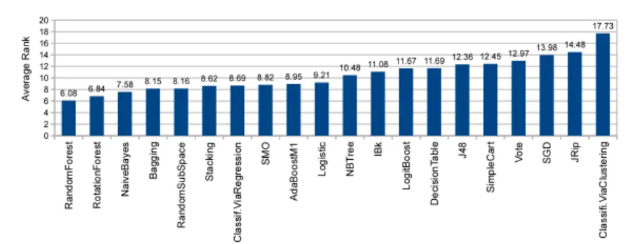
Alternative distance functions could also be used but we will show later (Eq. 11) that the Spearman’s distance has some convenient mathematical properties. To get a feeling about what an average ranking is in our meta-learning problem, Figure 4 shows an example of the average ranks of 20 algorithms over 466 datasets.
In the ART algorithm, we use the median value of a meta-feature’s range as the binary split point to split the dataD, the current partition, into two sub-partitions
D+andD−. The best split point is determined to be the one that maximises theR2
statistic: R2=1− ∑ L l=1∑n (l) i=1d(y(li),zˆ(l)) ∑Ll=1∑n (l) i=1d(y(li),zˆ(D)) , (8)
whereLis the number of partitions, andn(l) is the number of examples in partition
l.R2is originally designed to measure the proportion of the spread explained by the differences between the two partitions [30]. There are two special cases: if the sample central rankings of different partitions are equal, such as
ˆ
z(1)=...=zˆ(L), (9) thenR2=0 implies that partitioning is not necessary; if there is only one distinct ranking within each partition, and they are not all the same between partitions, then
R2=1. Here we estimateR2and employ it as a heuristic for ART induction. Next, we will derive an “one-step” formula for calculatingR2without calculating the distance between the central ranking and the other rankings in a partition.
At inner nodes, ART tests two partitionsD+andD−so we haveL=2, and we can rewrite Eq. (8) to:
R2=1−∑ n(D+) i=1 d(y(D +i) ,zˆ(D+)) +∑n (D−) i=1 d(y(D −i) ,zˆ(D−)) ∑n (D+) i=1 d(y(D +i) ,zˆ(D)) +∑n(D−) i=1 d(y(D −i) ,zˆ(D)) =1−n (D+)d¯(D+) Spearman+n(D −)¯ d(D − ) Spearman n(D+) ¯ d(D)Spearman+n(D−)¯ dSpearman(D) , (10) whereD=D+∪D−.
For rank data the average distance is also a proper measure of spread ˆα: ˆαSpearman≡ ¯
dSpearman [30]. [2] and [30] present a convenient mathematical result for Spearman’ distance (a brief derivation is given in the Appendix):
ˆ
αSpearman=
m(m+1)(2m+1) 3 −2||y||¯
2. (11)
Here we replace ¯dSpearmanwith ˆαSpearman, and rewrite Eq. (10) to:
R2=1−n (D+) ˆ α(D +) Spearman+n (D−)ˆ α(D −) Spearman n(D+) ˆ αSpearman(D) +n(D−)αˆ(D) Spearman =1−n (D+)αˆ(D+) Spearman+n(D −) ˆ α(D −) Spearman n(D)αˆ(D) Spearman . (12)
Combining everything together, we can computeR2(Eq. 8) efficiently:
R2=1−n
(D+)(h−2||y¯(D+)||2) +n(D−)(h−2||y¯(D−)||2)
n(D)(h−2||y¯(D)||2) , (13) whereh=m(m+1)(2m+1)
3 .
4.3 ART’s Stopping Criterion
In order to prevent overfitting, a stopping criterion is usually used to determine if it is worthwhile to split the current node. A natural stopping criterion can be introduced by adding a regularization parameterθ, e.g., ART will stop growing the current node if:
R2(bestSplit)≥θ,θ∈(0,1], (14) Another stopping criterion is the minimum number of examples at a leaf node,γ. Settingγ to a small number usually outperform trees using largerγvalues when the tree algorithm is used as the base learner for random forests [10]. ART uses both of these criterias to limit tree sizes.
4.4 ART Forests and Rank Aggregation
We use the random forests framework described in [10] for ART Forests induction. Algorithm 2 shows the pseudocode. An ART forest is grown as follows:
1. The training set is a bootstrap sample from the original training set;
2. An integeru is set by the user. At each node,ufeatures are selected at random and the node is split on the best feature among the selectedu;
Algorithm 2Approximate Ranking Tree Forests (ART Forests)
Input:
T(number of ART to use)
D(training data, an×mdata matrix);
u(number of features to use, defaultlog2M+1,Mis the total number of features) C(splitting and stopping criterions, details are given in Sec 4.2 and 4.3) ARTensemble←/0
fori=1toTdo
Di←getBootstrapSample(D)
ARTi←ART(Di,u,C)
ARTensemble←ARTensemble∪ARTi
end for
ReturnARTensemble
For prediction, when a test feature vectorxis put down each tree, it is assigned the average ranking of the rankings at the node it stops at. The average ranking of these over all approximate ranking trees in the forest is the predicted ranking for
x. Alternative rank aggregation methods, such as other types of Borda count, graph theory models, or binary linear programs, might perform better, at the expense of higher computational cost, and will be investigated in future research.
5 Experiment Setup and Results
This experimental comparison investigates two related questions.
– The first question concerns the new meta-feature generation method: can it con-sistently improve the performance of known meta-learners?
– The second question concerns the new algorithm: are ART Forests competitive with current state-of-the-art rankers?
In this paper, we focus on the performance of meta-learning for algorithm rank-ing on binary classification datasets only. Previous studies were limited by the small number of available datasets, usually fewer than 100 datasets were used in reported meta-learning experiments. To be able to draw statistically significant conclusions, we chose to use as many datasets as possible from various public data sources, in-cluding the UCI1, StatLib2, KDD3 and WEKA4repositories. In total slightly more than 1,000 classification and regression datasets were collected. However, due to the varying quality of the public datasets, not all of them could be used directly. After removing duplications and very small datasets (less than 10 instances), and convert-ing multiple-class classification data – by keepconvert-ing only the top two majority classes – and regression data – by using the mean as a binary splitting point to transform the
1 http://archive.ics.uci.edu/ml/ 2 http://lib.stat.cmu.edu/ 3 http://kdd.ics.uci.edu/
Fig. 4 Sorted average ranks of the 20 algorithms over 466 datasets based on PSO-optimised performances. This list can be transformed to a ranking, e.g., (optimised) RandomForest is ranked 1, RotationForest 2,..., ClassificationViaClustering 20. The ranking can be seen as a default ranker over the 466 datasets.
numeric target into a binary target –, a total of 466 datasets was obtained for experi-mentation. Also, to speed up our experiments we capped the number of instances in larger datasets to a maximum of 5,000 instances, using stratified random sampling.
5.1 EA-Based Performance Estimation
For simplicity and in order to speed up experiments, many previous meta-learning experiments have estimated algorithm performance using some pre-specified default parameter settings across all base-level learners. We claim that this approach is bound to be suboptimal in practice because to be able to make useful predictions, most algo-rithms have to be optimised separately for each specific dataset. Technically, predict-ing the full combination of algorithm plus optimal parameter settpredict-ings is not feasible. We therefore propose an intermediate approach, where we assume that a procedure is available for optimising each algorithm for each dataset, and then predict the ranking of the optimised algorithms. Given a new dataset, the recommended ranking is based on the assumption of using optimal parameter settings. These actual optimal param-eter settings would have to be computed for each top-ranked algorithm through the exact same optimisation process that was used for meta-learning.
The parameter optimisation procedure used here is based on evolutionary algo-rithms. Grid-search would be an alternative, but based on recent research [33], EA-based techniques seem more efficient. Specifically, we employ the particle swarm op-timisation (PSO) based parameter selection technique described in [16, 39]. Although EA-based performance estimation is more appropriate, it is time-consuming, espe-cially for large datasets. Therefore, as mentioned above, large datasets were down-sampled to 5,000 instances. In this paper, meta-learning is used to rank 20 supervised machine learning algorithms, all of which are implemented in WEKA [19]. When generating the meta-dataset from the 466 datasets, for each of the 20 algorithms, we manually specify parameters and their respective value ranges for PSO to optimise. Taking the support vector machine algorithm as an example, we set PSO to optimise the kernel type, all relevant kernel parameters, and the complexity constant.
Fig. 5 Percentage of improvement of the best AUC performance among 20 PSO-optimised algorithms for each dataset over the same 20 algorithm using their default parameters. Sorted by percentage of improve-ment over 466 datasets.
The class distributions of the 466 datasets vary a lot, with some of the datasets being very skewed, which can cause high variance on zero-one loss estimation. Con-sequently, we choose the area under the receiver operating characteristic curve (AUC) metric as the main performance measure, as it is less affected by class skew. We run the 20 algorithms, with PSO-based parameter optimisation, on the 466 binary classi-fication datasets and use 10-fold cross-validation based AUC scores for ranking gen-eration. Building up this meta-dataset is the most expensive part of our meta-learning experiment: it took roughly three weeks, or about 6,000 single-core CPU hours, to complete on two 2.8GHz 16G RAM PCs, with 6 threads running on each machine. Figure 5 shows the percentage of improvement of the best AUC score among the 20 PSO-optimised algorithms for each dataset over the best AUC score of the same 20 algorithms using their default parameters. The result demonstrates the benefit of us-ing the performances of optimised algorithms for generatus-ing algorithm rankus-ings. We claim this is a more appropriate experimental setting for meta-learning than simply using a fixed set of parameters for every dataset.
5.2 Meta-Learners (Rankers) in Comparison
We test the new pairwise meta-rule based meta-features with different meta-learners. In total 7 rankers are used for our experiments.
DefaultRanker—The default ranker follows a very simple yet powerful philoso-phy: if an algorithm has worked well on previous datasets, then it is likely to be used as the first algorithm to try on a new dataset. So, the default ranker used in our exper-iments is simply using the average rank of each algorithm over all the training data. Thus the ranking predicted by the default ranker is always the same for every test dataset, which is the average ranking of the training examples. This ranker can also be seen as a special case of an ART model with only one node. One distinguishing feature of the algorithm ranking problem is that this average-ranking-based default ranker is relatively strong compared to other common preference learning problems, such as movie or book recommendation, or survey data involving human subjects.
k-NN—Thek-NN ranker, as described in Section 2, uses standard Euclidean dis-tance and we setk= 15 (we will show later that 15 is a relatively good value for our problem).
LRT—The label ranking trees ranker, we use the WEKA-LR5implementation with default parameters. LRT is based on the Mallows model for rank data.
RPC—The RPC ranker, which uses the ranking by pairwise comparison algo-rithm proposed in [20]. We use the default setting of the RPC implementation in WEKA-LR in which the logistic regression algorithm is used as the base learner.
PCTR—The PCTR ranker, which is the predictive clustering trees for ranking (PCTR) ranker [40]. The minimum number of instances at a leaf node is set to 15.
AdaRank—The AdaRank ranker uses 100 PCTR rankers as its base models and the minimum number of instances at a leaf node is set to 30 (to simulate a relatively weak learner as in [43, 29]). Please note that boosting algorithms can stop early so the final AdaRank ensemble might not have exactly 100 base models.
ARTForests—The ARTForests ranker, where we use 100 approximate ranking trees for ART Forests, and the minimum number of instancesγ at a leaf node is set to 1 for each ART (using smallγ such as 1 leads to a good bagging ensemble as suggested in [10]); The “pruning” parameterθis set to 0.95.
5.3 Evaluation of Ranking Accuracy
We assess ranking accuracy by comparing the rankings predicted by a ranker for a given dataset with the corresponding target rankings. Given two sets ofm-value rankings:T= [T1,T2, ...,Tm−1,Tm]andP= [P1,P2, ...,Pm−1,Pm], which are targets and predictions, respectively, and lettingdi2= (Ti−Pi)2, the following ranking evaluation metrics and functions are used in our experiments.
Spearman’s Rank Correlation Coefficient (SRCC)—SRCC is defined as: ρSRCC=1− 6∑
m i=1di2
m(m2−1), (15)
which assesses how well the relationship between the true and predicted rankings can be described using a monotonic function [25].
Weighted Rank Correlation—WRC is defined as: ρW RC=1−6∑
m
i=1di2((m−Ti+1) + (m−Pi+1))
m4+m3−m2−m . (16) The WRC metric puts more weight on the top candidates. It has been used for meta-learning in [37, 32].
Loose Accuracy—The loose accuracy (LA@X) measurement considers ranking accuracy of the topX candidates only. LA@1 is also called the restricted accuracy metric, returning a count of 1.0 if the top one prediction is correct, and otherwise returning 0. Similarly, LA@3 returns a count of 1.0 if one of the predicted top three candidates matched the true top one, and again returning 0 otherwise. LA has been used for meta-learning in [23]. We report results for LA@1, LA@3 and LA@5.
Normalized Discounted Cumulative Gain—Discounted cumulative gain (DCG) is a measure of effectiveness of a search engine algorithm or related applications by
using a graded relevance scale of items in a result list [22]. The gain is accumulated from the top of the list to the bottom with the gain of each result discounted at lower ranks. The DCG@X is defined as: DCG@X=∑Xi=1 2
gi−1
log2(i+1), where gi is a grade value. The Normalized DCG at positionXis defined as:
NDCG@X=DCG@X×(IDCG@X)−1, (17)
here IDCG is the ideal DCG atX. We report results for NDCG@1, NDCG@3 and NDCG@5.
The actual evaluation scores for the above ranking evaluation functions of each ranker were estimated based on multiple runs of train/test split evaluations. We use the average scores obtained from 10 runs of 90% vs. 10% train/test evaluation for result visualization. For each run, 419 (90% of 466) datasets were randomly selected for building a meta-learning system using the corresponding ranker, and the remaining 47 datasets were used for testing.
To avoid information leaking, we make sure that when rule based meta-features are used by a ranker, the rules are generated using only the corresponding training meta-dataset of each run.
5.4 Experimental Results
We present and analyse two sets of experimental results. One is a comparison of meta-feature sets based onk-NN performance curves; the other one is a comparison of ranking performances of multiple rankers on two meta-feature sets.
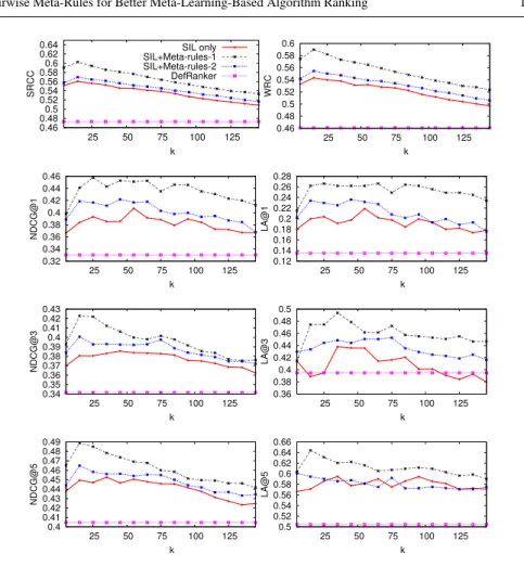
Figure 6 shows the performances of the k-NN ranker using three meta-feature sets under different numbers of nearest neighbors (k). The performance of the de-fault ranker is also included. Overall,kvalues between 10 and 20 usually produce relatively good performance across all eight ranking metrics. Regarding the choice of meta-feature sets, we can see thatk-NN using the SIL+Meta-rules-1 set outperforms the SIL-only and the SIL+Meta-rules-2 meta-feature sets when appropriatekvalues are chosen. Taking the LA@1 metric as an example, the bestk-NN performance is about 0.26, which means that on average, if an optimalkvalue is used, the probability for thek-NN ranker to predict correctly the best algorithm to use from 20 algorithms is 26%, where the default ranker achieves about 14%, and random guessing would only result in 1/20 = 5%. The LA@3 and LA@5 metrics behave similarly. Regard-ing the other five metrics, they all usually outperform the baseline, albeit to varyRegard-ing degrees, always clearly depending on a proper choice of the value ofk.
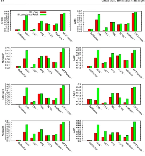
With the second set of results, we compare different rankers on two sets of meta-features: the SIL-only set and the rules-1 set. For simplicity, we use SIL+Meta-rules to refer the SIL+Meta-SIL+Meta-rules-1 set. Figure 7 shows the performances of the seven rankers (with and without using the meta-rules) on the eight metrics. A “*” besides a ranker’s name means the SIL+Meta-rules set is significantly better than the SIL-only set (using a pairedt-test significance level of 0.05). In total, the SIL+Meta-rules set significantly wins 38 out of 48 (about 79.1%) comparison tests across all rankers (please note that the default ranker is not counted since it does not use any meta-features). Overall, we can see that the ART Forests ranker with the SIL+Meta-rules
Fig. 6 Comparison of meta-feature sets byk-NN curves. Higher scores are better.
set consistently produces performance gains for all different metrics, and is placed as the best ranker for 7 out of 8 metrics. Although increasing ART Forests’ ensemble size may further improve its performance, using 100 as a default setting seems to work well for our experiments.
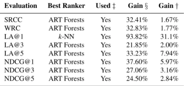
Table 1 shows a summary of the top one ranker for each metric and how much per-formance gain the respective ranker can achieve. We can see that all the best rankers used the SIL+Meta-rules set. The greatest performance gain (93%) over the default ranker is from thek-NN ranker on the LA@1 measurement. The “Gain §” values show how much improvement the top rankers using the SIL+Meta-rules meta-feature set can achieve over the default ranker; and the “Gain†” values show how much im-provement the Meta-Rule method (Method 1) introduced in this paper can achieve over the respective best rankers using the SIL-only meta-feature set.
In terms of runtime, the RIPPER-based pairwise meta-rules method on average takes 30 seconds to generate rulesets for 190 algorithm pairs. Figure 8 shows the run-time of different rankers. We can see that the ART Forests algorithm (with 100 ART
Fig. 7 Comparison of meta-feature sets by ranker performances.
Fig. 8 Single-core runtime in seconds including both training and prediction stages.
models) is relatively efficient compared with other state-of-the-art rankers. When rapid modeling is required for an application, thek-NN ranker is a reasonable al-ternative because it is fast and relatively accurate.
Table 1 Summary of the top one ranker performances under different ranking evaluation metrics and functions.Used‡: meta-rules (SIL+Meta-Rule set) is used, or not.Gain§: performance gain of the best ranker over the default ranker.Gain†: performance gain of the best ranker using the SIL+Meta-Rule set over the same ranker using the SIL-only set.
Evaluation Best Ranker Used‡ Gain§ Gain†
SRCC ART Forests Yes 32.41% 1.67%
WRC ART Forests Yes 32.83% 1.77%
LA@1 k-NN Yes 93.82% 31.1%
LA@3 ART Forests Yes 21.85% 2.00%
LA@5 ART Forests Yes 33.23% 7.94%
NDCG@1 ART Forests Yes 37.60% 5.97% NDCG@3 ART Forests Yes 27.06% 3.16% NDCG@5 ART Forests Yes 24.50% 2.84%
6 Discussions and Future Work
In this section, we discuss the limitations of the proposed techniques and future work for extending and improving the system.
For the pairwise meta-rule method, although the RIPPER algorithm works well, we believe that alternative rule learners are still worth investigating. An important direction for future work is the design of an efficient rule learner for generating small numbers of high quality pairwise meta-rules, as the number of pairwise rule models required increases quadratically with the number of algorithms to rank. Therefore, the training and the output complexity of the chosen rule learner is critical to the scalability of the proposed method. Ifzis the average number of rules returned by the rule learner for one pair of algorithms, then the total number of pairwise meta-rule based meta-features generated formalgorithms is zm(m2−1). Consequently, when using the pairwise meta-rule method, the number of meta-features grows quadrati-cally with the number of algorithms to rank. Some algorithms, like the novel ART Forests algorithm proposed here, scale well with larger number of features, whereas for some of the alternative rankers both runtime and ranking performance might suf-fer from a larger number of features, especially if there are strong correlations present among these features. To overcome this problem, in future work, we will investigate: (1) rule pruning techniques for reducing the total number of pairwise meta-rules; (2) rule set fusion techniques, such as group-wise meta-rules. Another interesting fu-ture direction would be using the predicted rank differences, or at least the actual posterior probabilities of the binary problem, instead of the purely boolean pairwise meta-features, for improved ranking performance.
Regarding the details of the ART algorithm, in this paper we only considered and evaluated using the median value of a meta-feature’s dynamic range as abinarysplit point. A future work direction would be comparing this to both alternative split point selection and to multi-way splitting strategies.
In this paper, we employed the EA-based parameter selection technique, which is a relatively expensive approach for generating meta-dataset. In the literature, there
are some attempts to use meta-learning itself for the task of parameter selection. [38] and [1] have shown promising results using meta-learning for selecting the kernel type and kernel parameters for support vector machines. There is also previous work that proposed hybrid systems combining meta-learning and optimisation techniques [33, 18, 14]. These systems could be used as alternative parameter selection proce-dures for the meta-learning experiment setup proposed in the this paper. In Section 5.1, we mentioned that predicting the full combination of algorithm plus optimal pa-rameter settings is not feasible. While this is technically true, [27, 28] has introduced the active testing based meta-learning framework that is able to return good param-eter setting together with the recommended algorithm. In their experiments, a set of 292 algorithm-parameter combinations was evaluated. The techniques described in the current paper could probably also be applied to meta-learning for parameter rec-ommendation of single learning algorithms, but this needs to be verified in a future experimental study.
7 Conclusions
We have introduced a new approach for generating meta-features to meta learning. The main difference between our method and stacking is given in Section 3. We have introduced a specialised meta-learning algorithm, based on the random forests frame-work [10], for predicting algorithm rankings, and provided both a theoretical and an empirical analysis. Unlike previous work, experiments in this paper were based on a much larger collection of publicly available datasets and a novel, more appropriate meta-learning experiment configuration, which systematically explores the space of parameter values of the algorithms to be ranked.
Our experimental results indicate that the pairwise meta-rule generation method (Method 1) consistently improves the performances of different ranking approaches to meta-learning. The new ART Forests ranker is always among the top rankers across all ranking metrics and functions we have tested. The success of the proposed meth-ods and algorithms on the meta-learning problem studied in this paper suggests the applicability of the new techniques to a wider range of meta-learning problems. Ad-ditional materials can be found at http://www.cs.waikato.ac.nz/~qs12/ml/
meta/.
Appendix: A brief derivation of Eq. 11
Here we give the core steps of the derivation. For a more detailed derivation of the intermediate steps, we refer the reader to [2, 30].
LetQmbe the set of allm×mpermutation matrices, wheremis the number of objects (e.g., algorithms) to rank. The setsSm (in Eq. 4) andQmare in one-to-one correspondence:
Q(y)em=y,Q(y)∈Qm,y∈Sm, wheree0m= [1,2,3, ...,m]. For example,Qi j=1 iffyi=j.
Letdbe a Hoeffding distance of the form, d(x,y) = m
∑
i=1 a(xi,yi) =tr(Q(x)∆Q(y) 0 ).For Spearman distance (which is a form of Hoeffding distance): ∆ =fm10m+1mfm0 −2eme0m,
wherefm0 = [1,22,32, ...,m2]and 10m= [1,1,1, ...,1]. The spread in Eq. 11 is calculated as:
ˆ αSpearman=∑ n i=1∑nj=1d(y(i),y(j)) n2 = ∑ni=1∑nj=1tr(Qi∆Q0j) n2 =tr(Mˆ∆Mˆ 0),
where ˆMis the marginal matrix ([30]) and ˆM1m=Mˆ01m=1m. Since it is well know that the sum of the squares of integers 12+22+32+...+m2=m(m+1)(2m+1)
6 , therefore ˆ αSpearman=2(10mfm)−2(Meˆ m)0(Meˆ m) = m(m+1)(2m+1) 3 −2||y||¯ 2. References
1. Shawkat Ali and Kate A. Smith-Miles. A meta-learning approach to automatic kernel selection for support vector machines. Neurocomputing, 70(13):173 – 186, 2006.
2. Mayer Alvo, Paul Cabilio, and Paul D. Feigin. Asymptotic theory for measures of concordance with special reference to average kendall tau. The Annals of Statistics, 10(4):pp. 1269–1276, 1982.
3. H. Bensusan, C. Giraud-Carrier, and C. Kennedy. A higher-order approach to meta-learning. Technical report, University of Bristol, 2000.
4. G. Biau. Analysis of a random forests model. Journal of Machine Learning Research, 13:1063–1095, April 2012.
5. Hendrik Blockeel, Luc De Raedt, and Jan Ramon. Top-down induction of clus-tering trees. InProceedings of the Fifteenth International Conference on Ma-chine Learning. Morgan Kaufmann Publishers Inc., 1998.
6. P. Brazdil, J. Gama, and B. Henery. Characterizing the applicability of classi-fication algorithms using meta-level learning. InProceedings of the European Conference on Machine Learning, 1994.
7. P. Brazdil, C. Giraud-Carrier, C. Soares, and R. Vilalta. Metalearning: Applica-tions to Data Mining. Springer, 2009.
8. P. Brazdil, C. Soares, and J. P. Da Costa. Ranking learning algorithms: Using ibl and meta-learning on accuracy and time results. Mach. Learn., 50(3):251–277, March 2003.
9. L. Breiman. Bagging predictors. Machine Learning, 24(2):123–140, August 1996.
10. L. Breiman. Random forests. Machine Learning, 45:5–32, 2001.
11. Weiwei Cheng, Jens H¨uhn, and Eyke H¨ullermeier. Decision tree and instance-based learning for label ranking. InProceedings of the 26th International Con-ference on Machine Learning (ICML-09), pages 161–168, Montreal, Canada, June 2009.
12. Weiwei Cheng and Eyke H¨ullermeier. Instance-based label ranking using the mallows model. In Workshop Proceedings of Preference Learning, Antwerp, Belgium, 2008.
13. W. W. Cohen. Fast effective rule induction. InProceedings of the 12th Interna-tional Conference on Machine Learning. Morgan Kaufmann, 1995.
14. P.B.C. de Miranda, R.B.C. Prudencio, A.C.P.L.F. Carvalho, and C. Soares. Com-bining a multi-objective optimization approach with meta-learning for svm pa-rameter selection. In2012 IEEE International Conference on Systems, Man, and Cybernetics, pages 2909–2914, 2012.
15. Bradley Efron and Robert J. Tibshirani.An Introduction to the Bootstrap. Chap-man & Hall, 1993.
16. H. J. Escalante, M. Montes-y Gmez, and L. E. Sucar. Particle swarm model selection.Journal of Machine Learning Research, pages 405–440, 2009. 17. C. Giraud-Carrier. Metalearning - a tutorial. InProceedings of the 7th
Interna-tional Conference on Machine Learning and Applications. Morgan Kaufmann, 2008.
18. Taciana A.F. Gomes, Ricardo B.C. Prudłncio, Carlos Soares, Andr L.D. Rossi, and Andr Carvalho. Combining meta-learning and search techniques to select parameters for support vector machines. Neurocomputing, 75(1):3 – 13, 2012. 19. M. Hall, E. Frank, G. Holmes, B. Pfahringer, P. Reutemann, and I. H. Witten.
The weka data mining software: an update. SIGKDD Explor. Newsl., 11(1):10– 18, 2009.
20. Eyke H¨ullermeier, Johannes F¨urnkranz, Weiwei Cheng, and Klaus Brinker. Label ranking by learning pairwise preferences. Artif. Intell., 172(16-17):1897–1916, November 2008.
21. Norbert Jankowski, Wlodzislaw Duch, and Krzysztof Grabczewski, editors.
Meta-Learning in Computational Intelligence, volume 358 ofStudies in Com-putational Intelligence. Springer, 2011.
22. K. J¨arvelin and J. Kek¨al¨ainen. Cumulated gain-based evaluation of ir techniques.
ACM Trans. Inf. Syst., 20(4):422–446, October 2002.
23. A. Kalousis.Algorithm Selection via Meta-Learning. PhD thesis, Department of Computer Science, University of Geneva, 2002.
24. A. Kalousis and M. Hilario. Model selection via meta-learning: a comparative study. International Journal on Artificial Intelligence Tools, 10(04):525–554, 2001.
25. Maurice G. Kendall.Rank correlation methods. Griffin, 1970.
26. R. Leite and P. Brazdil. Predicting relative performance of classifiers from sam-ples. InProceedings of the 22nd International Conference on Machine Learning, 2005.
27. Rui Leite, Pavel Brazdil, and Joaquin Vanschoren. Selecting classification algo-rithm with active testing on similar datasets. InProceedings of the 5th
Interna-tional Workshop on Planning to Learn, 2012.
28. Rui Leite, Pavel Brazdil, and Joaquin Vanschoren. Selecting classification algo-rithms with active testing. In Petra Perner, editor,Machine Learning and Data Mining in Pattern Recognition, volume 7376 ofLecture Notes in Computer Sci-ence, pages 117–131. Springer Berlin Heidelberg, 2012.
29. Hang Li. Learning to rank for information retrieval and natural language process-ing.Synthesis Lectures on Human Language Technologies, 4(1):1–113, 2011. 30. John I. Marden.Analyzing and Modeling Rank Data. Chapman & Hall, 1995. 31. B. Pfahringer, H. Bensusan, and C. Giraud-Carrier. Meta-learning by
landmark-ing various learnlandmark-ing algorithms. InProceedings of the 17th International Con-ference on Machine Learning, 2000.
32. Joaquim Pinto da Costa and Carlos Soares. A weighted rank measure of correla-tion. Australian & New Zealand Journal of Statistics, 47(4):515–529, 2005. 33. M. Reif, F. Shafait, and A. Dengel. Meta-learning for evolutionary parameter
optimization of classifiers. Machine Learning, 87:357–380, 2012.
34. C. Schaffer. A conservation law for generalization performance. In Proceed-ings of the 11th International Conference on Machine Learning, pages 259–265. Morgan Kaufmann, 1994.
35. Floarea Serban, Joaquin Vanschoren, Jorg-Uwe Kietz, and Abraham Bernstein. A survey of intelligent assistants for data analysis. ACM Computing Surveys, 2012.
36. K. A. Smith-Miles. Cross-disciplinary perspectives on meta-learning for algo-rithm selection. ACM Comput. Surv., 41(1):6:1–6:25, January 2009.
37. C. Soares. Learning Ranking of Learning Algorithms. PhD thesis, Department of Computer Science, University of Porto, 2004.
38. Carlos Soares, Pavel B. Brazdil, and Petr Kuba. A meta-learning method to select the kernel width in support vector regression.Machine Learning, 54(3):195–209, 2004.
39. Q. Sun, B. Pfahringer, and M. Mayo. Full model selection in the space of data mining operators. InProceedings of the 14th International Conference on Ge-netic and Evolutionary Computation Conference Companion, 2012.
40. L. Todorovski, H. Blockeel, and S. Dzeroski. Ranking with predictive clustering trees. InProceedings of the 13th European Conference on Machine Learning. Springer, 2002.
41. D. H. Wolpert. Stacked generalization.Neural Networks, 5:241–259, 1992. 42. D.H. Wolpert and W.G. Macready. No free lunch theorems for optimization.
IEEE Transactions on Evolutionary Computation, 1(1):67–82, apr 1997. 43. J. Xu and H. Li. Adarank: a boosting algorithm for information retrieval. In
Proceedings of the 30th International Conference on Research and Development in Information Retrieval. ACM, 2007.