A Dissertation by HAOBO REN
Submitted to the Office of Graduate Studies of Texas A&M University
in partial fulfillment of the requirements for the degree of DOCTOR OF PHILOSOPHY
August 2005
A Dissertation by HAOBO REN
Submitted to the Office of Graduate Studies of Texas A&M University
in partial fulfillment of the requirements for the degree of DOCTOR OF PHILOSOPHY
Approved by:
Chair of Committee, Tailen Hsing Committee Members, Raymond J. Carroll
Suojin Wang Qi Li
Head of Department, Simon J. Sheather
August 2005 Major Subject: Statistics
ABSTRACT
Functional Inverse Regression and Reproducing Kernel Hilbert Space. (August 2005)
Haobo Ren, B.S., Peking University; M.S., Peking University
Chair of Advisory Committee: Dr. Tailen Hsing
The basic philosophy of Functional Data Analysis (FDA) is to think of the observed data functions as elements of a possibly infinite-dimensional function space. Most of the cur-rent research topics on FDA focus on advancing theoretical tools and extending existing multivariate techniques to accommodate the infinite-dimensional nature of data. This dis-sertation reports contributions on both fronts, where a unifying inverse regression theory for both the multivariate setting (Li 1991) and functional data from a Reproducing Kernel Hilbert Space (RKHS) prospective is developed.
We proposed a functional multiple-index model which models a real response vari-able as a function of a few predictor varivari-ables called indices. These indices are random elements of the Hilbert space spanned by a second order stochastic process and they con-stitute the so-called Effective Dimensional Reduction Space (EDRS). To conduct inference on the EDRS, we discovered a fundamental result which reveals the geometrical associa-tion between the EDRS and the RKHS of the process. Two inverse regression procedures, a “slicing” approach and a kernel approach, were introduced to estimate the counterpart of the EDRS in the RKHS. Further the estimate of the EDRS was achieved via the transfor-mation from the RKHS to the original Hilbert space. To construct an asymptotic theory, we introduced an isometric mapping from the empirical RKHS to the theoretical RKHS, which can be used to measure the distance between the estimator and the target. Some general
computational issues of FDA were discussed, which led to the smoothed versions of the functional inverse regression methods. Simulation studies were performed to evaluate the performance of the inference procedures and applications to biological and chemometrical data analysis were illustrated.
To my wife, Caixia Zhao
ACKNOWLEDGMENTS
I want to express my sincerest appreciation to my advisor, Dr. Tailen Hsing, who brought me into the exciting world of functional data analysis, showed me the amazing idea of inverse regression and continuously supported me to complete my Ph.D. degree during the past few years. His broad knowledge and strong intuition in probability and statistics, and foremost his great personality have set an example to me for my future career.
Special thanks are due to all my committee members: Dr. Raymond J. Carroll, who encouraged me on my theoretical studies during my preliminary exam and his workshop in 2004, Dr. Qi Li, who discussed with me many interesting problems in statistics and econometrics, and Dr. Suojin Wang, who taught me the theory of sampling, resampling and asymptotics. I gratefully acknowledge Dr. Michael Sherman for his willingness and time to substitute for Dr. Carroll, to attend and participate in my defense. Dr. Sherman introduced me to spatial statistics in the fall of 2000, which was instrumental in preparing for my thesis. Further I wish to mention Dr. Randy L. Eubank, who introduced the beautiful theory of reproducing kernel Hilbert space to the seminar of functional data analysis in the spring of 2003, which I attended.
I am indebted to my extended family including my relatives living in China for their patience and understanding while I was studying in Texas A&M University. My greatest debt is to my wife, who helped me type this thesis and continued to provide love and support through this process.
TABLE OF CONTENTS
Page
ABSTRACT . . . iii
DEDICATION . . . v
ACKNOWLEDGMENTS . . . vi
TABLE OF CONTENTS . . . vii
LIST OF FIGURES . . . ix CHAPTER I INTRODUCTION . . . 1 II LITERATURE REVIEW . . . 3 2.1 FDA . . . 3 2.2 IR . . . 9
2.3 RKHS with Applications in Probability and Statistics . . . 13
III A FUNCTIONAL MULTIPLE-INDEX MODEL . . . 15
3.1 A Second Order Multiple-Index Model . . . 15
3.2 Some Facts of RKHS . . . 16
3.3 Probabilistic Substructure—Between IR and RKHS . . . 21
IV STATISTICAL FRAMEWORK IN RKHS . . . 32
4.1 Discretization . . . 32
4.2 IR Procedures in RKHS . . . 33
4.3 Asymptotic Studies in RKHS . . . 35
V INVERSE OF LO ´EVE’S ISOMETRY – TRANSFORMATION FROM RKHS TO L2SPACE . . . 48
5.1 Parzen’s Methods . . . 48
5.2 Weiner’s Improved Iteration . . . 50
5.3 Direct Approach . . . 51
6.1 Smoothing . . . 54
6.2 Inverse of Covariance Operator . . . 58
VII EMPIRICAL STUDIES . . . 61
7.1 Monte Carlo Experiments . . . 61
7.2 Data Analysis . . . 72
7.3 IR of Hybrid Data . . . 79
VIII CONCLUSIONS . . . 89
REFERENCES . . . 91
LIST OF FIGURES
FIGURE Page
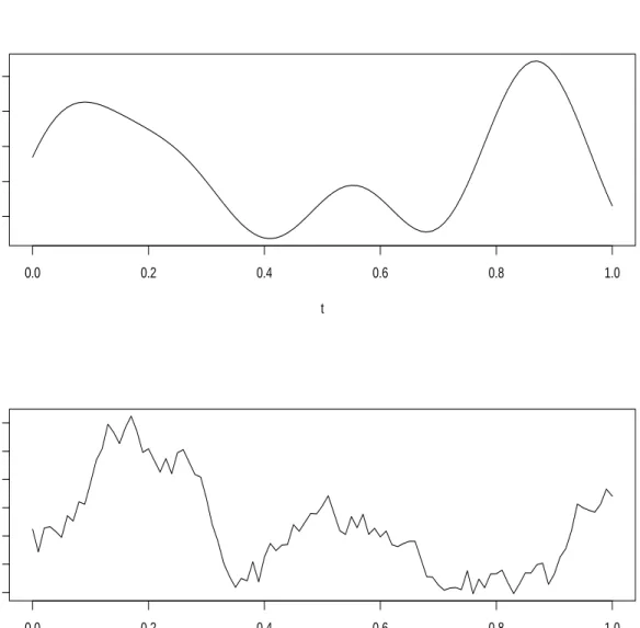
1 Illustrations of the Three-Component Process and Brownian Motion. . . 64
2 Illustrations of Fractional Brownian Motions. . . 65
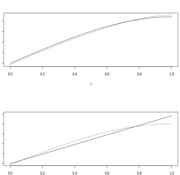
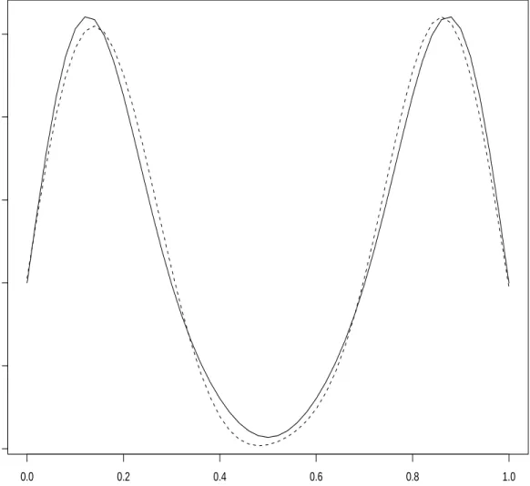
3 FSIR Estimation for Experiment 1. . . 66
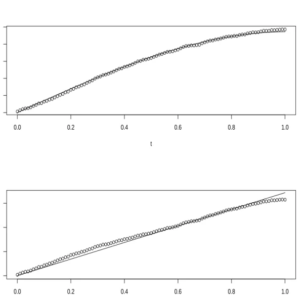
4 The Randomly Sampled Bm Trajectories in Experiment 2. . . 68
5 Smoothed FSIR Estimation for Experiment 2. . . 69
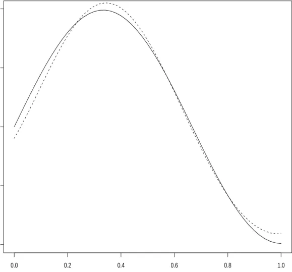
6 FSIR Estimation for Experiment 3. . . 70
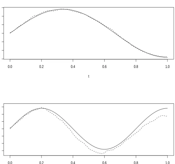
7 Smoothed FKIR Estimation for Experiment 4. . . 71
8 Estimated Index Coefficient Functions for a Two-Index Model. . . 73
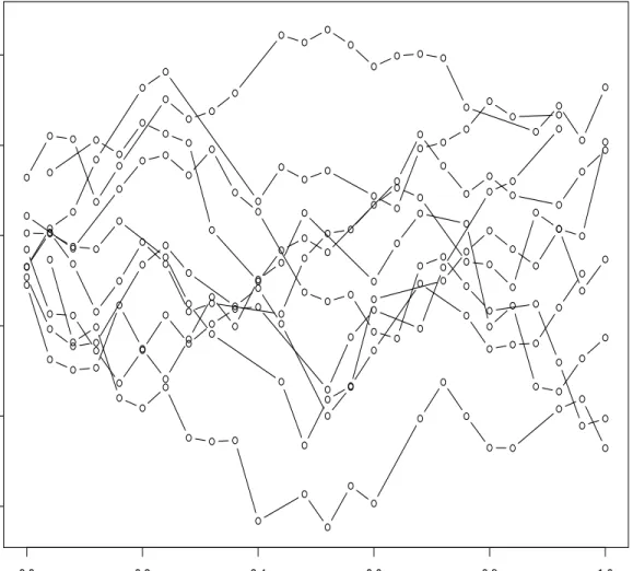
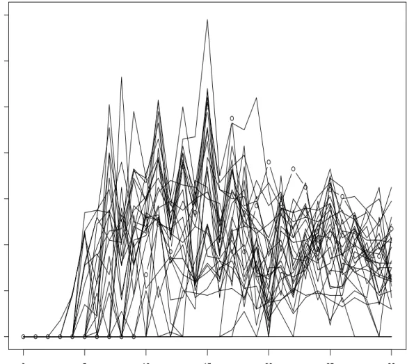
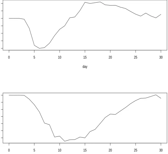
9 The Reproductive Trajectories of 30 Medflies. . . 74
10 The Index Coefficient Functions in Modeling the Lifetime of Medflies. . . . 76
11 The Estimated Link Function in Modeling the Lifetime of Medflies. . . 77
12 The Single Index Coefficient Function in Modeling Lifetime Indicator of Medflies. . . 78
13 The Spectra of 30 Selected Samples. . . 80
14 The Index Coefficient Functions in Modeling the Tecator Data. . . 81
15 The Estimation in Modeling the Tecator Data. . . 82
16 The True Indices Versus the Predicted Indices for the Hybrid Data. . . 85
17 The Single-Index Coefficient Function in Modeling the Hybrid Teca-tor Data. . . 86
CHAPTER I
INTRODUCTION
Stochastic statistics, longitudinal data analysis (LDA) and functional data analysis (FDA), are three closely related areas and comprise a trilogy in modern statistics. Stochastic statis-tics, including time series analysis and spatial statisstatis-tics, makes inference based on a long observed trajectory of a random process. Longitudinal data often refer to many short series of records, for which various parametric models combined with nonparametric smoothing are the major approaches. Compared to stochastic statistics and LDA, FDA is a more gen-eral area of research which is nonparametric in nature, while parametric modeling can be done in abstract function spaces to capture the functional features of the data.
FDA is largely motivated by the emergence of an abundance of functional data. With the rapid development of accurate instruments, measurement could be taken continuously over a period of time to produce data in functional form. Statisticians tend to compare functional data with longitudinal data, and view functional data as densely observed longi-tudinal data, similar to the generalization from repeated measurement model to longilongi-tudinal data analysis. However, the concept of functional data has brought more profound, creative and revolutionary ideas to statistics.
The basic philosophy of FDA is to think of each data function as a single observa-tional unit due to the precise and frequent sampling procedure, although in reality it is only possible to observe the function at a finite number of grid points. As a result, FDA should
This dissertation follows the style and format of the Journal of the American Statistical Association.
be considered in function spaces which are likely to be infinite-dimensional. This leads to considerations which are substantially different from those of the traditional multivariate analysis. Another aspect of FDA is to treat every observation element as a sample path from a specific stochastic process, hence stochastic inference is relevant.
Most of the current research on FDA focuses on two directions: to create advanced theoretical tools and to adapt existing multivariate techniques to infinite-dimensional func-tional data. Reproducing Kernel Hilbert Space (RKHS) is an effective and profound device for statistical analysis involving infinite dimensional data objects, while inverse regression (IR) is a renowned and brilliant idea in multivariate analysis, both of which are recently in-troduced to the FDA context. This research will focus on the functional inverse regression (FIR) from the RKHS prospective.
This dissertation is organized as follows. Chapter II will give a literature review on FDA, IR and RKHS, respectively. In Chapter III, we present a functional multiple-index model and explore its probabilistic structure. The estimation framework within RKHS is described and the associated asymptotic theory is constructed in Chapter IV. Chapter V investigates the transformation from the RKHS to the Hilbert space of the stochastic pro-cess. Chapter VI will discuss some computational issues in FDA and propose the smoothed versions of the estimation. Empirical studies including simulation and data analysis are re-ported in Chapter VII. Chapter VIII gives a brief conclusion.
CHAPTER II
LITERATURE REVIEW
This research comprises three components: Functional Data Analysis (FDA), Inverse Re-gression (IR) and Reproducing Kernel Hilbert Space (RKHS). In this chapter, we shall make an overview of current research topics on FDA and IR and recall the history of RKHS.
2.1 FDA
More and more data nowadays can be easily collected in the form of curves or images. Statistical methods for analyzing such data are termed “functional data analysis”, a term coined by Ramsay and Dalzell (1991). The basic philosophy of FDA is to think of each observed curve or image as a single observation rather than a collection of individual ob-servations. In terms of the different philosophy and methodology on how to treat these data, the current FDA research can be largely classified into three schools: English, French and Stochastic. The relationship among FDA, longitudinal data analysis and time series analysis will also be discussed in this review.
2.1.1 English School
The methodologies of the English school are represented by Ramsay and Silverman (1997) with the applications illustrated in Ramsay and Silverman (2002). Smoothing techniques dominate this school. Each sampling element is viewed as a smooth function, and the key step is to convert raw, discretely observed, data into genuine functional elements by various smoothing techniques including basis function (Fourier, wavelets and B-splines), localized smoothing (kernel and local polynomial regression) and roughness penalty or regularization approach (smoothing splines). There is a vast literature in the field of statistical smoothing,
see the monographs by Eubank (1999), Green and Silverman (1994), Simonoff (1996) and Wand and Jones (1995) for an overview of these nonparametric techniques.
So far, considerations on processing and displaying of functional data have focused on pattern or structure search and registration (Kneip and Gassar 1992, Gassar and Kneip 1995, Ramsay and Li 1997, Liu and Muller 2003, and Rossi, Delannay, Conan-Guez and Verleysen 2005), the estimation of mean and covariance structure (Rice and Silver-man 1991), principal component analysis (SilverSilver-man 1996), canonical correlation analysis (Leugrans, Moyeed and Silverman 1993) and linear discriminant analysis (Hastie, Buja and Tibshirani 1995).
As in multivariate data analysis, various types of linear models are the most-studied topics. Obviously, there are many different varieties of functional linear models since we can entertain a number of different combinations of functional and scalar components in both the response and predictor variables. The simplest and most-studied one has a scalar response and functional predictor. Hall and Horowitz (2004) and Cai and Hall (2005) discussed the large sample properties of functional linear regression. Crambes (2005) pro-posed total least square approach for functional linear measurement error models. James (2002) and M¨uller and Stadtm¨uller (2004) provided some extensions of generalized lin-ear models and quasi-likelihood method to functional predictors. Escabias, Aguillin-ear and Valderrama (2004) introduced the functional principal component logistic regression.
Recently, James and Siverman (2005) introduced an adaptive functional model which extends generalized linear models, generalized additive models and projection pursuit re-gression to handle functional predictors. It takes the form
g(E(y|x)) =β0+ r
∑
k=1 fk µZ x(t)βk(t)dt ¶ ,where x is the predicting curve, y is an exponentially distributed scalar response, respec-tively, g is the link function,βk’s are coefficient functions, and fk’s are the suitably smooth
curves as in additive models or projection pursuit regression models. A penalized maxi-mum likelihood estimation approach is used to fit both fk’s andβk’s.
On the other hand, for works involving both functional response and predictors, Mal-fait and Ramsay (2003) considered the historical linear model
y(t) =α(t) +
Z S
0 x(s)β(s,t)
ds+ε(t),
where x(s),s∈[0,S] and y(t),t ∈[0,T] are the exploratory and response curves, respec-tively, ε is the error process and β is the bivariate regression coefficient function. They applied the finite element method to estimateβ.
2.1.2 French School
The name of FDA is twofold: the data is functional and the analytical method uses func-tional analysis. The French FDA school applies funcfunc-tional analysis extensively. The basic observational unit is treated more abstractly as an element in a function space and most functional analysis concepts and tools such as operator theory can help form the mathemat-ical foundation of functional data analysis.
Dauxois, Pousse and Romain (1982) was one of the pioneering works in FDA which constructed an asymptotic theory for functional principal component analysis by using pure analysis and measure-theoretic language. Fine (2003) explored the similar theory for canonical correlation analysis in a Hilbert space using operator and tensor approach. Bosq (1991) proposed a first order Hilbertian autoregressive model in H, where H is a real separable Hilbert space equipped with norm k · kand inner product h·,·i, to describe the dynamics of a sequence{Xt}of H-valued random variables such that
Xt=ρ(Xt−1) +εt, t∈Z,
where{εt} is an H-white noise, which means that εt’s are H-valued, identically and
Eεt=0, andρis a symmetric compact linear operator on H withkρkB(H)<1, where B(H)
is the space of linear bounded operator on H. Additionally, assume that EkX0k4<∞. Define the covariance operator C of X0by C=E(X0⊗X0), and the cross-covariance operator D of(X0,X1)by D=E(X0⊗X1), where⊗is the tensor product in H, meaning for a,b∈H, a⊗b∈B(H), such that
a⊗b(f) =ha,fib, ∀f ∈H. By the strict stationarity one can derive that D=ρC.
To estimateρ, the inverse of C must be treated properly since it could be either non-existing or unbounded. The following projection method was then developed in the paper. Let(λk,νk),k∈N,be the eigenvalues and eigenfunctions of C arranged in the order
ofλ1≥λ2≥ ··· ≥0. Define the subspace of H, VK=span(ν1,···,νK), and the associated
projector by ΠK = Pro j VK = K
∑
k=1 νk⊗νk.The projected covariance and cross-covariance are C(K) =ΠKCΠK and D
(K) =ΠKDΠK,
respectively. We then consider an estimatorρK =D(K)C(−K1) ofρ.
This idea was borrowed directly by Cardot, Ferraty and Sarda (1999) to estimateΨin the functional linear model
Y =Ψ(X) +ε,
where Y andεare real random variables, X is a H-valued random variable with EkXk2<∞, and Ψ is a real linear continuous functional on H. This approach also formed the basis of functional principal component regression. In the follow-up studies, Cardot, Ferraty and Sarda (2003) addressed the computational implementation by penalized B-spline, and Cardot, Ferraty, Mas, and Sarda (2003) discussed the testing of hypothesis of H0:Ψ=0
with certain computing issues addressed in Cardot, Goia and Sarda (2004). Goia (2003) also considered the model selection problem.
Among other topics, Cardot (2000) investigated the smoothing effect in functional principal component analysis, Cardot, Crambes and Sarda (2004) proposed the functional quantile regression, Cardot and Sarda (2005) studied the functional generalized linear model, and Cueva, Febrero and Fraiman (2002) handled the functional linear model with functional response.
2.1.3 Stochastic School
The stochastic school treats each functional sample unit as a realization from a random process. Strictly speaking, this is different from classical stochastic statistics (Rao 2000) in which the inference is based on only one realization of a stochastic process. In FDA, the covariance function is crucial for many analyses, therefore the Karhunen–Lo´eve expansion (Ash and Gardner 1975) is one of the most useful tools in this approach.
Karhunen–Lo´eve expansion: Let{X(t),t ∈[a,b]} be a L2 process (E(X(t)2<∞ for all t∈[a,b]) with zero mean and continuous covariance K. Let {en,n=1,2, . . .} be an
orthonormal basis for the space spanned by the eigenfunctions of the nonzero eigenvalues of the integral operator associated with K, with en taken as an eigenvector corresponding
to the eigenvalueλn. Then
X(t) =
∞
∑
n=1Znen(t), t∈[a,b],
where Zn=RabX(t)en(t)dt, and the Znare orthogonal random variables with E(Zn) =0 and
E(Z2
n) =λn. The series converges in L2to X(t), uniformly in t.
Huang, Quek and Phoon (2001) studied the performance of the truncated Karhunen– Lo´eve expansion method in the simulation of a stochastic process. Yao, M¨uller, Clifford, Dueker, Follett, Lin, Buchholz and Vogel (2003) used a smoothed version of the truncated
Karhunen–Lo´eve expansion to represent each sampled curve. The functional canonical correlation analysis was implemented by He, M¨uller and Wang (2002) and an application could be found in He, M¨uller and Wang (2004). Preda and Saporta (2005a) considered functional partial least squares and also gave an application in Preda and Saporta (2005b).
All schools focus on the adaptation of standard multivariate techniques to FDA. So far, principal component analysis (Silverman 1996), canonical correlation analysis (Leurgans, Moyeed and Silverman 1993 and He et al. 2002), and linear model (Cardot et al. 1999) have been successfully considered in functional data analysis context. In a nutshell, the approach of the English school is very effective in the practical data analysis, while the approach of the French school gives functional data analysis a sound theoretical basis. It will be beneficial to study FDA from all three perspectives.
2.1.4 A Trilogy in Modern Statistics
FDA, LDA and time series analysis (TSA, or more generally, the stochastic statistics, which includes spatial statistics) constitute a trilogy of modern statistics. In terms of data struc-ture, time series data are collected usually as a long series of observations, longitudinal data are measured repeatedly over time giving rise to many short time series, while functional data have more general forms. Theoretically, LDA and TSA are in the field of parametric statistics, while the essence of functional data is infinite-dimensional and hence nonpara-metric statistics has a large role in FDA.
TSA focuses on modeling the dependence and prediction using mainly parametric approaches; an example is the classical autoregressive moving average (ARMA) model. In LDA, the challenge is the apparent nonstationarity of the repeated measurements for each subject. With the assumption of independence among the subjects, the inferences about the common covariance matrix can be achieved by borrowing strength across many subjects, which is the idea of pooled TSA.
A heuristic and insightful comparison on LDA and FDA from the smoothing perspec-tive could be seen in Rice (2004). Many FDA studies are longitudinal-data driven. This is analogous to the relation between repeated measures model and LDA. The typical linear model in LDA could be viewed as a functional linear model with both functional response and covariates,
Y(t) =β(t)TX(t) +ε(t),
which has been studied extensively in FDA. Specifically, the mixed effects model from LDA is transplanted to functional linear model and combined with smoothing or basis splines from the FDA side, which generates a powerful tool for both LDA and FDA. Brum-back and Rice (1998) and Rice and Wu (2001) made contribution in this direction, Chiou, M¨uller and Wang (2003) and Guo (2002) studied the functional mixed effect models in more depth. It becomes a trend that more FDA techniques are introduced to LDA, for ex-ample, functional principal component analysis has been applied to LDA (Besse, Cardot and Ferraty 1997, James, Hastie and Sugar 2000 and Yao, M¨uller and Wang 2005) and a functional multiplicative effects model was proposed to study longitudinal behavior in bi-ology science (Chiou, M¨uller, Wang and Carey 2003). Between TSA and FDA, the works in Bosq (1991, 2000) introduced some advanced techniques in TSA to FDA. Laukaitis and Raˇckauskas (2002) illustrated an application of functional autoregressive model in financial time series data.
2.2 IR
IR has been an active research topic for about fifteen years since its introduction in Li (1991). Recently, functional data analysts started working on it. In this section, the research of both multivariate and functional IR will be reviewed.
2.2.1 Multivariate Multiple-Index Model and IR
The seminal paper Li (1991) proposed the following multiple-index model which is a regression-type semiparametric model,
y= f(β′1x,β′2x, . . .,β′px,ε)
where x and βi’s belong to Rd, ε and x are independent of each other, 1≤ p ≤d and f : Rp+1 7→R. Call each β′ix an index, βi the index coefficient vector, and f the link
function. The number of indices, coefficient vectors and the link function are all unknown. One important implication of the model is that the projection of the d-dim explanatory variable onto the p-dim subspace
B=span(β′1x,β′2x, . . . ,β′px),
captures all we need to know about y, or, in probability language, y and x are independent of each other given (β′1x,β′2x, . . .,β′px). The central goal of the model is to estimate the so-called effective dimension-reduction (EDR) space, span(β1,β2, . . .,βp).
There are many papers on multiple-index type models. H¨ardle and Stocker (1989) investigated the method of average derivative estimate (ADE), which has been developed in a series of works; for example, Donkers and Schafgans (2003) used outer product of derivatives, and Hristache, Juditsky, Polzehl and Spokoiny (2001) proposed an iterative improvement. The single-index model (p=1) attracted the most attention. Among many works Hristache, Juditsky and Spokoiny (2001) developed ADE for single-index model, Naik and Tsai (2000) studied the performance of partial least square method, and Yu and Ruppert (2002) used penalized splines for partially linear single-index model.
On the other hand, to extend the idea of EDR space, Cook (1998) defined B as the dimension-reduction subspace, and then further developed the concept of central subspace in theoretical and graphical tools.
To explore the geometrical structure of the multiple-index model, Li (1991) added a crucial condition,
E(b′x|β′1x,β′2x, . . .,β′px)∈span{β′1x,β′2x, . . .,βp′x}, for ∀b∈Rd.
See Hall and Li (1993) for more detailed discussion of the condition. For a model satisfying this condition, the space span(Σβ1,Σβ2,Σ. . .,βp)contains the centered IR curve E(x|y)−
E(x), where Σ=Cov(x). This implies that the principal component analysis or eigen-decomposition of∆can achieve the estimation of the EDR space. Then how to estimate∆ orΣ−∆becomes the central problem, where∆=Cov[E(x|y)].
Li (1991) proposed the now well-known sliced IR (SIR) which can be proceeded by five steps based on data(xi,yi), i=1,···,n,
1. Center and standardize x, zi=Σˆ−n1/2(xi−¯x), i=1,···,n,where ˆΣn is the estimate of
Σ.
2. Divide the range of y into S slices, I1,···,IS.
3. Estimate E(z|y) by sliced mean, ¯zs = ns1 ∑ni=1ziI(yi∈Is), s=1,···,S, where ns =
∑n
i=1I(yi∈Is),
4. Estimate Cov(E(z|y))by the weighted covariance matrix, ˆV = 1n∑Ss=1ns¯zs¯z′s.
5. Implement the principal component analysis of ˆV .
Duan and Li (1991) and Li (1997) presented more delicate results for analyzing single-index regression by SIR, Hsing and Carroll (1992) and Zhu and Ng (1995) derived the large sample properties of SIR based onΣ−∆, Chen and Li (1998) illustrated the features of SIR. Schott (1994), Ferr´e(1997 and 1998) discussed the determination of the number of indices in SIR. Carroll and Li (1992) applied SIR to measurement error models, and Becker and Fried (2002) made a direct use of SIR in high-dimensional time series analysis.
For data analysis, He, Fang and Xu (2003) analyzed mass spectra data by combining SIR and classification tree, Gannoun, Girard, Guinot and Saracco (2004) combined SIR and a kernel estimation of conditional quantile to estimate reference curves in clinical studies.
For other IR approaches, Zhu and Fang (1996) proposed a kernel regression to estimate E(x|y) and also gave an asymptotic result. Gather, Hilker and Becker (2002) evaluated the sensitivity of SIR to outliers and Gather, Hilker and Becker (2001) provided a robust version of SIR. Fung, He, Liu and Shi (2002) implemented SIR by B-spline and canonical correlation to estimate ∆. Bura and Cook (2001) introduced a parametric IR which fitted E(x|y)via a multivariate linear regression. Naik and Tsai (2005) proposed the constrained IR in the presence of linear constraints on parameters. A more innovative idea based on SIR was in Xia, Tong, Li and Zhu (2002) which generated a minimum average conditional variance estimation inspired by the SIR, ADE and local linear smoothers.
A complementary method of SIR termed sliced average variance estimates (SAVE) was introduced in Cook and Weisberg (1991). Its asymptotic theory was provided in Gan-noun and Saracco (2003) and an application to microarray data was reported in Bura and Pfeiffer (2003).
2.2.2 Functional Inverse Regression
In the functional SIR proposed in Ferr´e and Yao (2003) under setting of the French school, the model, assumption and procedures were all parallel to Li (1991) by translating the terms from the linear algebra to functional analysis. The model is
Y = f(hβ1,XiH,hβ2,XiH, . . . ,hβp,XiH,ε),
whereβ’s and X belong to H=L2([a,b])with E(kXk2)<∞. With the assumption E(hβ,XiH|hβ1,XiH, . . . ,hβp,XiH ∈span{hβ1,XiH, . . . ,hβp,XiH} for ∀β∈H,
the spectral decomposition ofΓ−X1ΓE(X|Y) can estimate span{β1, . . . ,βp}, where ΓZ is the
covariance operator of a stochastic process Z ∈
H
. The SIR procedure can be imple-mented in a way that is similar to the multivariate case to estimateΓE(X|Y). However,Γ−X1 is problematic due to its unboundedness. The projection technique in Bosq (1991) was then applied here.Another functional IR method under the same setting as above was considered by Amato, Antoniadis and Feis (2004), in which E(X|Y)was estimated by wavelet smoothing. Both Li, Aragon, Shedden and Agnan (2003) and Setodji and Cook (2004) applied IR to the functional response and multivariate input model:
y(t) =g(β1(t)′x, . . . ,βp(t)′x) +ε(t).
The former used basis presentation and the latter used k-means approach for slicing. These two papers originally intended to extend the univariate IR to multivariate response data, which had been done in Hsing (1999) by nearest neighbor IR.
2.3 RKHS with Applications in Probability and Statistics
RKHS methods have been employed by probabilists and statisticians for at least fifty-five years. With the applications done by of the machine learning community, it has become an active topic of research in statistics. Recent works also bring strong evidences of its promising role in FDA.
The theory of RKHS was originated from complex analysis, developed in integral equations and bounded-value problems, and matured into the present form in the landmark paper Aronszajn (1950). It was introduced into the probability world by Lo´eve (1948), which built the famous Lo´eve’s isometry. Parzen (1959) introduced RKHS to statisticians; Parzen (1961a, 1961b) solved several crucial problems in signal analysis using this power-ful tool, providing a convincing evidence of the relevance of RKHS in time series analysis
and general stochastic inference. See Weinert (1982) for a collection of these papers. Bar-ton and Poor (1990) and Nuzman and Poor (2001) gave two applications to robust signal analysis and self-similar processes, respectively. Wahba’s well-known work in the 1970’s formulated the mathematical foundation of the nonparametric smoothing with spline func-tions using RKHS (Wahba 1990). Gu (2002) developed tensor product smoothing splines by further application of RKHS. Vapnik’s statistical learning theory (Vapnik 1995) includ-ing the support vector machine revitalized the interest of RKHS in nonparametric statistics; the kernel-based algorithms are among the most exciting research topics in both signal anal-ysis and statistics today. For other application of RKHS, see Berlinet and Thomas–Agnan (2004).
In FDA context, the use of RKHS can be seen throughout Ramsay and Dalzell (1991). The function space H is partitioned into a direct sum of subspaces H1 and H2 for two linear operators, L and B, such that H1=ker(L), H2=ker(B) and H =H1⊕H2, where H1 contains the structural components and is usually of finite dimension, H2contains the residual components and is usually infinite dimensional. Based on this partitioning, further analyses including the representation of the discrete observation by a function in H was accomplished by RKHS or Wahba’s spline theory.
Eubank and Hsing (2005) brought RKHS to FDA under the setting of the stochas-tic school. By Lo´eve’s isometry and tensor product of RKHS, both the concept and the computations of canonical correlations were extended to general stochastic processes.
In the remainder of the dissertation, we will present a new functional multiple-index model and propose inverse regression approaches from the RKHS perspective. This method-ology is closer in spirit to the practice of the stochastic school, and at the same time it uses the functional analysis language from the French school, and incorporates smoothing tech-niques from the English school.
CHAPTER III
A FUNCTIONAL MULTIPLE-INDEX MODEL
In this chapter, a multiple-index model related to a second order stochastic process will be proposed in the first section. To explore the geometrical structure of the model, we will give some basic facts of the reproducing kernel Hilbert space (RKHS) in Section 3.2. Then Section 3.3 provides the relationship between the RKHS and inverse regression.
3.1 A Second Order Multiple-Index Model
Let {Xt,t ∈T} be a real-valued zero-mean, second order stochastic process defined on
some probability space(Ω,
F
,P), where the index set T is assumed to be a separable metric space. Here and elsewhere, a second-order process or L2 process refers to a process such that E(|Xt|2)<∞for all t∈T . See Ash and Gardner (1975) for background knowledge onsecond-order stochastic processes.
Define the Hilbert space L2X generated by the process in the following way. First let span{Xt,t ∈T}, be the set of finite linear combinations of random variables of the form
Xti for ti∈T . Further let span{Xt,t∈T}be the closure of span{Xt,t∈T}in L2(Ω,
F
,P).Then L2X is defined to be the space containing elements in span{Xt,t ∈T} and equipped
with the inner product
hU,ViL2
X =E(UV).
Thus, L2X contains the random variables attainable by linear operations on Xt and their L2
limits.
Let us now define the following conditions in whichξ1, . . . ,ξpare elements in L2X and
(IR1) Y and X are conditionally independent of each other givenξ1, . . . ,ξp.
(IR2) For anyξ∈L2X,
E(ξ|ξ1, . . . ,ξp)∈span{ξ1, . . . ,ξp} a.s..
A particularly relevant situation for which (IR1) holds is the multiple-index model Y = f(ξ1, . . . ,ξp,ε), (3.1)
whereεis a random error independent of the process {Xt}, eachξ′ix is called an index and
f the link function. The number of indices, indices and the link function are all unknown. Condition (IR2) holds if the joint distribution of any finite collection of elements from LX2 is spherically symmetric, which would be the case if, for instance,{Xt}is a Gaussian
process.
The goal of the model is to estimate the so-called effective dimension-reduction (EDR) space, a subspace of L2X,
LX2,e=span{ξ1, . . . ,ξp} ⊂L2X,
which is equipped with the inner products of L2X.
So far, the set-up is analogous to Li (1991), however, we need more advanced theory for the RKHS to explore the structure of this model. Before doing so, we will briefly review the notion of RKHS.
3.2 Some Facts of RKHS
The general definition and common properties of an RKHS will be presented in this section, which could also be found in Aronszajn (1950), Pazern (1959), Kailath (1971), Wahba (1990), Luki´c and Beden (2001) (henceforth LB).
Definition III.1. A Hilbert space H is said to be a RKHS with reproducing kernel K, if each element of H is a function defined on some set T , and there is a bivariate function K on T ×T , having the following two properties:
(1) For all t ∈T , K(·,t)∈H
(2) For all t ∈T and f ∈H, f(t) =hf,K(·,t)iH
There are three components of a RKHS: the index set T , the Hilbert space H of func-tions, i.e. H ⊂RT, and the kernel function with the specific reproducing property in (2). We use the triple notation(T,H,K)or H(K,T)to denote a RKHS.
There are many nice properties of RKHS, mostly due to the existence of kernel. The first two properties are related to the alternative characterization and denseness of RKHS.
Property III.1. (Alternative Characterization)
In the RKHS, H(K,T), every evaluation functional is continuous, which means that for all t ∈T , the functional et with et(f) = f(t) for all f ∈H(K,T), satisfies |et(f)| ≤
MtkfkH for some Mt∈[0,∞).
Property III.2. (Denseness)
H(K,T) =span{K(·,t),t∈T}.
The following properties are related to the continuity and smoothness of the function. Property III.3. (Pointwise Continuity)
If{fn,n∈N,f} ⊂H(K,T), then
kfn−fkH −−−→
n→∞ 0=⇒ fn→ f for each point of T, as n→∞.
Property III.4. (Smoothness)
If K is a continuous bivariate function on T×T , then any f ∈H(K,T)is continuous on T .
The following properties are related to the kernel. Property III.5. (Uniqueness)
If K is the reproducing kernel of a RKHS, then K is non-negative definite and unique. Conversely, if K is a non-negative definite bivariate function on T ×T , a unique RKHS of real-valued function on T with K as its reproducing kernel can be constructed.
Definition III.2. (Non-negative and Positive Definite Functions)
A symmetric real-valued bivariate function K defined on T is said to be non-negative definite if for∀n∈N,{a1, . . . ,an} ⊂R,{t1, . . . ,tn} ∈T ,
n
∑
i,j=1aiajK(ti,tj)≥0,
and positive definite if the equality holds only when a1=a2=. . .=an=0. We shall use
K≥0 and K>0 to denote that K is non-negative and positive definite, respectively. Property III.6. (Sum of Reproducing Kernels)
The direct sum of two spaces(T,H1,K1)and(T,H2,K2)is also a RKHS. Denote it as (T,H,K), where H ={f = f1+f2,fi∈Hi,i=1,2}and K=K1+K2with norm defined by ∀f ∈H,kfk2H= min f=f1+f2 f1∈H1,f2∈H2 (kf1k2H1+kf2k 2 H2).
Property III.7. (Difference of Reproducing Kernels)
For two spaces (T,H1,K1) and (T,H2,K2), assume that K2−K1≥0, then H2⊃H1 and there exists a unique linear operator L : H27→H1such that for∀f ∈H2and g∈H1,
hf,giH
L satisfies
LK2(·,t) =K1(·,t), ∀t∈T, and L is a bounded self-adjoint and positive operator.
Definition III.3. (Dominance and nuclear dominance) Under the assumption of Prop-erty III.7, we say that K2 dominates K1 if K2−K1≥0, and denote it by K2≥K1. The operator L is called the dominance operator. If L is nuclear, i.e., it is trace-class operator, we say K2n-dominates K1, denote this by K2≫K1and L is called the nuclear dominance.
The following properties are related to the index set T . Property III.8. f ∈H(K,T) ⇐⇒ sup S sup ai |∑iaif(ti)|2 ∑i∑jaiajK(ti,tj) <∞, (3.2)
where the suprema are taken over all S={t1, . . . ,tn} ∈
F
={S⊂T : S is finite}and all reala1, . . . ,an, with n arbitrary, such that the denominator in (3.2) is not zero.
Property III.9. Let T be finite, and let the matrix determined by kernel K is nonsingu-lar. Then∀f,g∈H(K,T): kfk2K =
∑
t,s∈T f(t)f(s)K−1(t,s), hf,giK =∑
t,s∈T f(t)g(s)K−1(t,s), where K−1is the inverse of the matrix K.Let T be an index set and T1 ⊂T . For any f defined on T , let f|T1 stand for the
restriction of f to the subset of T1.
Property III.10. (Restriction of Index Set)
Suppose T1⊂T , let H1={f1= f|T1 : f ∈H}and K1=K|T1×T1, then H1=H(K1,T1) is a RKHS and
kf1kH1 = min f∈H f|T1=f1
Property III.11. (Approximation) Let T be either a countable or separable metric space, H(K,T)be a RKHS with K>0 and{Tn,n∈N}be a sequence of subsets of T that is
mono-tone increasing and ∪∞i=1Tn=T , we can define a sequence of spaces Hn=H(Kn,Tn)with
reproducing kernels Kn=K|Tn×Tn, then
(1) For any function f defined on T ,
kfnkHn ≤ kfn+1kHn+1,
where fn= f|Tn;
(2) For any f ∈H(K,T),
kfkH= lim
n→∞kfnkHn; (3) For any f which is continuous on T , then
lim
n→∞kfnkHn <∞=⇒ f ∈H(K,T). Property III.12. (Separability)
A topological structure of the index set could be induced by the kernel. For the RKHS (T,H,K), denote Ks=K(·,s), then dK(s,t) =kKs−Ktkdefines a pseudo-metric on T , and
we have
(1) K >0 implies that dK is a metric on T .
(2) If dK is a metric on T , then
(a)∀f ∈H(K,T)is dK-continuous.
(b)(T,dK)is separable iff H(K,T)is separable.
The last result concerns with the situation where both kernel and index set are varying. The following definition and property are excerpted form LB.
Definition III.4. (Hamel Basis and Hamel Set)
A set vα of linearly independent vectors in a vector space V is called a Hamel basis in V if{vα}spans V . Let V be the vector space spanned by{Kt,t∈T}, a set T0⊆T such that {Kt,t∈T0}is a Hamel basis of V will be called an K-Hamel subset of T .
Property III.13. Let H(R,T)be separable and let the kernel K be such that R≫K with dominance operator L. Let T0be an R-Hamel subset of T and S0={s1, . . .}be a dK-dense
subset of T0. Denote by Knand Rnthe matrices obtained by restricting the kernels K and R
to the set{s1, . . . ,sn} ⊂S0. Then
Tr(L) =Tr(KnR−n1),
where Tr(L) is the trace of operator of L.
The proofs of above properties could be found in Aronszajn (1950), Pazern (1959) and LB.
3.3 Probabilistic Substructure—Between IR and RKHS
The method of embedding of an abstract space into some RKHS is used extensively to stochastic processes. The central result is Lo´eve’s isometry. Consider a real-valued zero-mean L2process{Xt,t∈T}with
R(s,t) =E(XsXt) and Rt(·) =R(t,·), s,t∈T.
Then we can define the RKHS generated by {Xt,t ∈T}, which is just the RKHS with
reproducing kernel R:
H
X =span{Rt,t∈T}=the RKHS of{Xt,t∈T}=H(R,T).The inner product of H(R,T)is hf,giH X = ∞
∑
i,j=1 aibjR(si,tj), for f = ∞∑
i=1 aiRsi and g= ∞∑
j=1 bjRtj ∈H
X,which, by the reproducing property, satisfies
hf,RtiHX = f(t), t∈T.
Comparing this to the Hilbert space generated by the process, L2X, defined in Section 3.1, we see that L2X is isometrically isomorphic to
H
X, that is, there exists a one-to-one corre-spondence between the two spaces that preserves the inner products of the two spaces. Let Ψbe the corresponding isometry that maps L2X toH
X withΨ(Xt) =Rt, t∈T.
It follows thatΨ(η)(t) =E(ηXt), forη∈L2X and t ∈T . This mapping is called Lo´eve’s
isometry, which provides a duality between a stochastic process and its RKHS (Wahba 1990).
By this mapping, define the counterpart of EDRS in
H
X, a subspace ofH
X,H
X,e=ΨX(L2X,e) =span{Ψ(ξ1), . . . ,Ψ(ξp)} ⊂H
X,which is equipped with the inner products of
H
X and we simply call it the EDRS in RKHS. Motivated by the main theorem in Li (1991), we propose the following conjecture:The sample paths of conditional process, E(X|Y)∈
H
X,ea.s.At first glance, this may be proved using the same type of arguments as those in Li (1991) or Ferr´e and Yao (2003). However, we do not believe that this is the case. It turns that a more thorough study of the relationship between a RKHS and the sample paths of a stochastic process is required in the proof.
Parzen (1963) observed that almost all the sample paths of X lie outside
H
X if T is an infinite separable metric space and the R is continuous on T×T . Driscoll (1973) was the first paper to investigate the RKHS structure of the sample paths of a Gaussian process and gave sufficient conditions for the sample paths falling into a RKHS. Nearlythirty years later, LB summarized and generalized this category of problems. The following development is inspired by their results.
Defining the following conditions,
(P1) Let R be a continuous positive kernel on T×T ;
(P2) The sample paths of E(X|Y)are continuous with probability one. we have,
Theorem III.1. Assume that (P1), (P2), (IR1), and (IR2) hold. Then E(X|Y)∈
H
X,e a.s.Proof. To prove the theorem, a lemma is first stated.
Lemma III.1. Let S be a separable metric space. Let{Us,s∈S} be a L2-process on probability space (Ω,
F
,P) with mean function u and continuous covariance kernel K1. Assume that almost all the sample paths of U are continuous on S. Let K2be a continuous positive kernel on S×S such that with K2≫K1and u∈H(K2). Then P[U ∈H(K2)] =1.Proof of Lemma. Denote the metric of S by d and let S0 be a countable dense subset of S in d. Define
dK2(s,t) =kK2(s,·)−K2(t,·)kK2.
Since K2>0, it follows from Property III.12(1) that dK2 is a metric on S. For any s∈S, let
sn be a sequence of elements in S0which converges to s in S in the metric d. Then, by the
reproducing property,
dK22 (sn,s) =kK2(sn,·)−K2(s,·)kK22 =K2(sn,sn)−2K2(sn,s) +Ks(s,s)→0
by the continuity of K2. This shows that S0 is also dense in the metric dK2 so that S is also
Now enumerate the elements of S0and let Snbe the collections of the first n elements
according to the enumeration. Then Snis monotone increasing and limn→∞Sn=S0. Define f =U−u, K1,n=K1|Sn×Sn, K2,n=K2|Sn×Sn, fn= f|Sn, and Un=U|Sn. Observe that
E[kfnk2K2,n] =E(f ′ nK2−,n1fn) =E(tr(fn′K2−,n1fn)) =E(tr(fnfn′K2−,n1)) =tr[E(fnfn′)K2−,n1] =tr[cov(fn)K− 1 2,n] =tr(K1,nK− 1 2,n).
SincekfnkK2,n is monotone by (1) of Property III.11, it follows from the monotone
conver-gence theorem that
E[lim n→∞kfnk 2 K2,n] =nlim→∞tr(K1,nK −1 2,n). (3.3)
Note that since K2is nonsingular, T itself is an K2-Hamel subset of T . Let L be the dom-inance operator for
H
(K2)overH
(K1). By Property III.13 and the assumption K2≫K1, we havelim
n→∞tr(K1,nK −1
2,n) =tr(L)<∞.
It then follows from (3.3) that lim
n→∞kfnk 2
K2,n <∞ a.s.
By (3) of Property III.11, this implies that f ∈
H
(K2)a.s., and completes the proof. The proof of III.1 is accomplished in five steps as1. Let
H
E(X|Y)denote the RKHS of the process{E(Xt|Y),t∈T}, which is well-defined.Since
E[E(Xt|Y)] =E(Xt) =0,
and
it follows that {E(X(t)|Y),t∈T}is also a zero-mean, second order stochastic pro-cess, with covariance function
K(s,t):=Cov(E(Xs|Y),E(Xt|Y)), s,t∈T.
Thus, define L2E(X|Y)and the RKHS
H
E(X|Y) in the usual way. 2. Verify that dim(H
E(X|Y))≤p.By definition
L2E(X|Y)=span{E(Xt|Y),t ∈T},
and by (IR1) and (IR2),
E(Xt|Y) = E(E(Xt|Y,ξ1, . . . ,ξp)|Y) = E(E(Xt|ξ1, . . . ,ξp)|Y) = p
∑
i=1 ci,tE(ξi|Y) a.s.for some constants ci,t. It follows that
E(Xt|Y)∈span{E(ξi|Y), i=1, . . . ,p}.
Consequently,
L2E(X|Y)⊆span{E(ξi|Y), i=1, . . . ,p},
and hence
dim(L2E(X|Y)) =dim(
H
E(X|Y))≤p.Let ttt= (t1, . . . ,tm)′ ∈ Tm and aaa = (a1, . . . ,am) ∈Rm,m= 1,2, . . .. Writing XXX =
(Xt1, . . . ,Xtm)′, we have
var(aaa′XX) =X var(E(aaa′XXX|Y)) +E(var(aaa′XXX|Y)). Thus,
aa
a′(Rm−Km)aaa=E(var(aaa′XXX|Y))≥0,
where
Rm={R(ti,tj)}i,j=1,mand Km={K(ti,tj)}i,j=1,m.
This implies that R−K≥0, and we conclude that
H
X ⊇H
E(X|Y).Further, by Definition III.3, there exists a dominance operator L :
H
X →H
E(X|Y)such that
hf,giHX =hL f,giH
E(X|Y) for all f ∈
H
X and g∈H
E(X|Y).4. Verify that E(X|Y)∈
H
X a.s.Combining steps 2 and 3, we can conclude that the dominance operator L is a finite rank operator, hence L is a nuclear operator with tr(L)<∞. Since T is separable, and the continuity of R implies the L2-continuity of{Xt,t ∈T}, by the L2 convergence
property of conditional expectation,{E(X(t)|Y),t∈T}is also L2-continuous and so K is continuous. It then follows from Lemma III.1 that
5. Finally, prove that E(X|Y)∈
H
X,ea.s.. We will show thathE(X|Y),hiHX =0 for any h∈
H
X such thathh,Ψ(ξi)iHX =0, 1≤i≤p. (3.4)
Let ξ= Ψ−1(h)∈L2X. If h =Rt, then Ψ−1(h) =Xt. By the reproducing kernel
property,
hE(X|Y),hiHX =E(X|Y)(t) =E(Xt|Y) =E(ξ|Y).
In general if h=∑∞i=1diRti, thenξ=∑∞i=1diXti and
hE(X|Y),hiH X = ∞
∑
i=1 dihE(X|Y),RtiiHX = ∞∑
i=1 diE(Xti|Y) =E(ξ|Y).By the properties of conditional expectation and (IR1),
E(ξ|Y) =E(E(ξ|ξ1, . . . ,ξp,Y)|Y) =E(E(ξ|ξ1, . . . ,ξp)|Y).
It suffices to show that the above righthand side equals 0, which we now do. Since by (IR2), E(ξ|ξ1, . . . ,ξp) = p
∑
i=1 ciξifor some ci,1≤i≤ p, we have
E¡E2(ξ|ξ1, . . . ,ξp) ¢ = E Ã p
∑
i=1 ciξiE(ξ|ξ1, . . . ,ξp) ! = E Ã p∑
i=1 ciE(ξξi|ξ1, . . . ,ξp) ! = p∑
i=1 ciE(ξξi),which is equal to p
∑
i=1 cihΨ(ξi),Ψ(ξ)iHX = p∑
i=1 cihΨ(ξi),hiHX =0 by (3.4). Then E(ξ|ξ1, . . . ,ξp) =0 which implies E(E(ξ|ξ1, . . . ,ξp)|Y) =0.Hence the proof is complete.
♦
To apply the theorem to estimate the EDRS in RKHS,
H
X,e, we need to derive some corollaries from the theorem. By Theorem 3.1 of LB, since the sample paths of E(X|Y) belong toH
X, then R≥K implies that the covariance operator of E(X|Y)is well-defined and just equals to the dominance operator L, i.e.,L=E¡E(X|Y)⊗HX E(X|Y) ¢ , which is defined by L f =E(hE(X|Y),fiH XE(X|Y)), for f ∈
H
X.Since R≫K, L is a nuclear operator meaning a trace-class, symmetric and a non-negative operator. There are more properties of L:
Corollary III.1. L is degenerate in any direction orthogonal to
H
X,e. Proof. It follows from the theorem thatfor all s∈
H
X such that hs,ΨX(ξi)iHX =0,1≤i≤p. Hence 0 = E(hs,E(X|Y)i2HX) = E(hs,E(X|Y)iHXhs,E(X|Y)iHX) = E(hs,hs,E(X|Y)iHXE(X|Y)iHX) = hs,E(hs,E(X|Y)iHXE(X|Y))iHX = hs,LsiHX. ♦Corollary III.2. For the range of L, we have Im(L)⊂
H
X,e, where Im(L)is the range of L.Proof. For any f ∈
H
X and h⊥H
X,e, hL f,hiH X = E ¡ hE(X|Y),fiH XhE(X|Y),hiHX ¢ = E¡hE(X|Y),fiHX ·0¢ = 0. ♦In order to introduce functional sliced inverse regression in
H
X, we need another op-erator, ˜L= S∑
s=1 psE(X|Y ∈Is)⊗HXE(X|Y ∈Is), where Im(Y) =⊕S s=1Is and ps=Pr(Y ∈Is),s=1,···,S.Corollary III.3. For the sliced conditional sample path, if the sample paths of E(X|Y ∈ Is)are continuous with probability one, we have
E(X|Y ∈Is)∈
H
X, a.s.Proof. Let K and J be the kernels of E(X|Y) and E(X|Y ∈ Is), respectively. Note that
E(X|Y ∈Is) =E[E(X|Y)|Y ∈Is]. Then K−J≥0, which implies H(K)⊃H(J). Since
dim(H(J))≤dim(H(K))≤p, the dominance mapping from H(K)to H(J)is nuclear, by
Lemma III.1,
E(X|Y ∈Is)∈H(K)⊂
H
X.♦
Corollary III.4. ˜L is degenerated in any direction orthogonal to
H
X,e. Proof. Sincehs,E(X|Y)iHX =0
for all s∈
H
X such thaths,ΨX(ξi)iHX =0,1≤i≤p. h˜Ls,siH X = S
∑
s=1 pshE(X|Y ∈Is),si2HX = S∑
s=1 pshE[E(X|Y)|Y ∈Is],si2HX = S∑
s=1 psE2(hE(X|Y),siHX|Y ∈Is) = 0. ♦Corollary III.5. For the range of ˜L,
Im(˜L)⊂
H
X,e. Proof. For any f ∈H
X and h⊥H
X,e,h˜L f,hiHX = S
∑
s=1 pshE(X|Y ∈Is),fiHXhE(X|Y ∈Is),hiHX = S∑
s=1 pshE(X|Y ∈Is),fiHXE(hE(X|Y),hiHX|Y ∈Is) = 0. ♦CHAPTER IV
STATISTICAL FRAMEWORK IN RKHS
Theorem III.1 reveals the geometrical or probabilistic structure of the functional multiple-index model and facilitates the statistical inference based on inverse regression in the RKHS of the process. We will give the matrix version and computation related to the covariance operator in Section 4.1, two estimation procedures in Section 4.2, and the asymptotic results in Section 4.3.
4.1 Discretization
There are two reasons to consider discretization. Firstly, the covariance operators defined in most Hilbert spaces cannot be calculated directly. Secondly, in functional data analysis it is always the case that {X(t),t ∈T} is observed only on a discrete set of values of T , say Tq ={t1, . . . ,tq}. To apply the matrix language, we simply consider the rectangle
design, which means observing X= (X(t1), . . . ,X(tq))′ where t1< . . . <tq, and |ti+1−ti|,
i =1, . . . ,q−1, might be unequal but the same for all curves. This rectangle sampling scheme can be achieved by any representation method of the original sampling functional units. Then the following computation gives the matrix version for L. For f∈H(Rq,Tq),
Lqf = E ¡ E(X|Y)⊗RqE(X|Y) ¢ f = E³E(X|Y)hE(X|Y),fiRq´ = E¡E(X|Y)E(X|Y)′R−q1f¢ = [Cov(E(X|Y))R−q1]f.
Spectral decomposition in the discrete setting can be carried on by applying matrix optimization: max kfkRq=1h E¡E(X|Y)⊗RqE(X|Y) ¢ f,fiRq = maxhCov(E( X|Y))R−1 q f,fiRq f′R−q1f = maxf ′R−1 q Cov(E(X|Y))R−q1f f′R−q1f = maxg ′Cov(E(X|Y))R−1 q g g′g = max kgk=1g ′Cov(E(X|Y))R−1 q g.
Thus, the spectral decomposition of Lqcan be achieved by the eigen-decomposition for the
matrix Cov(E(X|Y))R−1
q . The above calculation also implies
argmax kfkRq=1 hE¡E(X|Y)⊗RqE(X|Y) ¢ f,fiRq =R1q/2argmax kgk=1 g′Cov(E(X|Y))R−q1g. (4.1) In data analysis, we will also encounter the problem that the covariance kernel is unknown, so that we have to estimate it in some way.
4.2 IR Procedures in RKHS
We have two approaches to estimate
H
X,e:If Im(˜L) =
H
X,e, the functional sliced inverse regression (FSIR) which generalizes Li (1991) can be used to estimate ˜L.If Im(L) =
H
X,e, we can implement the functional kernel inverse regression (FKIR), the extension of Zhu and Fang (1996) to estimate L.Then the spectral decomposition of the estimated operators gives an estimate of the EDR space in RKHS.
Let(Xi,Yi), i=1, . . . ,n, be a discrete sample of(X,Y). Estimate the covariance matrix
of X by ˆRq,n. Then the FSIR algorithm is
Step 0. Centering Xi’s.
Step 1. S-partition the range of Y to form{Is,s=1, . . . ,S}.
Step 2. ns=∑ni=1I(Yi∈Is), ˆps,n=nsn, and ˆµs,q,n=ns1 ∑ni=1XiI(Yi∈Is), s=1, . . . ,S.
Step 3. ˆ˜Lq,n=∑Ss=1pˆs,n ³
ˆµs,q,n⊗Rqˆ ,n ˆµs,q,n ´
. Where a⊗Rqˆ ,na=aa′Rˆ−q,1n.
Step 4. Implement the eigen-decomposition of ˆ˜Lq,n.
As the FSIR directly estimates the operator ˜L, the FKIR algorithm first estimates the conditional expectation E(X|Y)by kernel smoothing then the covariance of it:
Step 0. Centering Xi’s.
Step 1. Choose a kernel function and calculate ˆgq,n(y) = 1 nh n
∑
i=1 XiK µ Yi−y h ¶ and ˆ f(y) = 1 nh n∑
i=1 K µ Yi−y h ¶ . Step 2. Choose a small positive number b and computeˆ
fb(y) =max(b,fˆ(y)).
Step 3. Implement the Waston-Nadaraya type kernel estimation ˆ
mb,q,n(y) = ˆgq,n(y) ˆ fb(y) ,
where the bandwidth could be selected by cross-validation procedure. Step 4. ˆLq,n=1n∑in=1mˆb,q,n(Yi)⊗Rˆq,nmˆb,q,n(Yi).
4.3 Asymptotic Studies in RKHS
To prove the consistency of the estimators introduced in the previous section is a chal-lenging task. In the literature of functional data analysis, asymptotic results based on partially observed functional data have been rarely considered. For the present topic, un-der the assumption that each curve or sample unit is observed completely, in papers from the French school a number of asymptotic results were proved as the sample size n goes to infinity. We cannot try this approach, since even if observing the whole curves, i.e., the complete sample, {(Xi,Yi),i=1, . . . ,n}, we cannot prove that the estimator function,
ˆµs,n = 1n∑ni=1XiI(Yi ∈Is) from FSIR or ˆgn(y) = nh1 ∑ni=1XiK ³
Yi−y h
´
from FKIR falls into the RKHS of X . Actually, we have the following more general result.
Proposition IV.1. Let X1,···,Xnbe a sample from a zero-mean Gaussian process on a
real interval T , with a continuous positive covariance kernel R. The sample paths of X are continuous on T , a.s. Define Y=∑ni=1ciXi, where∑ni=1c2i >0. Then Y 6∈H(R)a.s.
Proof. Obviously, Y is a Gaussian process with continuous sample paths, and it is trivial to know that its covariance kernel is K=∑n
i=1c2iR. To apply Theorem 3 in Driscoll (1973),
let Tq={t1,···,tq}be a increasing series satisfying∪Tq=T . Define the restrictions Kq=
K|Tq×Tq and Rq=R|Tq×Tq, then lim q→∞tr(KqR −1 q ) = qlim→∞tr( n
∑
i=1 c2iRqR−q1) = lim q→∞q n∑
i=1 c2i = ∞.This completes the proof. ♦
On the other hand, in most classical works on application of RKHS in statistics, asymptotic results ar