Generating Diverse and Accurate Classifier
Ensembles Using Multi-Objective Optimization
Shenkai Gu
Department of ComputingUniversity of Surrey Guildford, Surrey, GU2 7XH
United Kingdom Email: [email protected]
Yaochu Jin
Department of ComputingUniversity of Surrey Guildford, Surrey, GU2 7XH
United Kingdom Email: [email protected]
Abstract—Accuracy and diversity are two vital requirements for constructing classifier ensembles. Previous work has achieved this by sequentially selecting accurate ensemble members while maximizing the diversity. As a result, the final diversity of the members in the ensemble will change. In addition, little work has been reported on discussing the trade-off between accuracy and diversity of classifier ensembles. This paper proposes a method for generating ensembles by explicitly maximizing classification accuracy and diversity of the ensemble together using a multi-objective evolutionary algorithm. We analyze the Pareto optimal solutions achieved by the proposed algorithm and compare them with the accuracy of single classifiers. Our results show that by explicitly maximizing diversity together with accuracy, we can find multiple classifier ensembles that outperform single classifiers. Our results also indicate that a combination of proper methods for creating and measuring diversity may be critical for generating ensembles that reliably outperform single classifiers.
Index Terms—Classifier ensemble, diversity, multi-objective optimization
I. INTRODUCTION
It has been shown, both theoretically and empirically, that classifier ensembles, which consist of multiple classifiers, can perform better than single classifiers [1], [2]. Usually, an ensemble is built in two steps, where the first step is to train a set of classifier members (also known as base classifiers) for a given task, and the second step is to combine these classifier members for the final prediction. It is found that both the accuracy of each ensemble member and the diversity among ensemble members are important for the overall performance of classifier ensembles [3], [4].
Brown [5] categorized existing methods for creating di-verse ensembles into four groups, namely: supplying differ-ent training data, employing differdiffer-ent learning algorithms, and initializing learning models with different weights or structures. Depending on whether the diversity is taken into account during ensemble construction, ensemble methods can be generally divided into two types, i.e., explicit and implicit methods [5]. For example, Bagging [6] is categorized as an implicit method, where it randomly samples training data to generate different training sets for each ensemble member, without measuring or ensuring diversity. Boosting [7] is an explicit method, that manipulates the probability of selecting
training data from the original training set in order to enhance diversity.
Since accuracy and diversity are very likely to conflict with each other, it is difficult to maximize both objectives at the same time, meaning that creating accurate and diverse ensem-bles is essentially a multi-objective optimization problem [8], [9]. To address this issue, previous work has aggregated multiple objectives into a scalar objective function [10], [11] and solved the problem with single-objective evolutionary algorithms. However, this requires the user to specify the hyper-parameter before learning, such that only one single solution can be found. As suggested in [9], using the Pareto-based multi-objective learning approach is the more natural way to solve this problem.
Regardless of how diversity is created, methods for building ensembles can be divided into two steps [12]–[17], i.e., first train multiple classifiers and then select a subset of them for constructing the ensemble. Theoretically, diversity should be measured among all members in an ensemble, which cannot be guaranteed if the ensemble members are selected one by one from a group of potential base classifiers. In order to address this issue, this paper proposes to combine the member generation and selection steps, where all members of an ensemble are generated simultaneously using a multi-objective evolutionary algorithm (MOEA), to optimize the accuracies of ensemble members and find groups of them, which have maximum diversity, at the same time. The main benefit of this approach is that diversity of the final solution can be accurately measured and the trade-off between accuracy and diversity of the whole ensemble can be taken into account during ensemble generation.
The remainder of the paper is organized as follows. Sec-tion II provides a brief descripSec-tion of the base classifiers used in this work. Section III details the proposed generation method. Section IV presents the experimental setup and the empirical results. Finally, Section V concludes this paper.
II. CLASSIFIERMODEL
Support vector machines (SVMs) use a discriminant hy-perplane to separate classes [18], [19], where the selected
hyperplane is optimized to maximize the distance between the nearest training points [18], [19].
Suppose we have a training set {(x1, y1), . . . ,(xn, yn)}, where xi are feature vectors and yi are the labels, i =
1,2, ..., n. The decision function can be formed as
f(x) = sgn n X i=1 yi↵iK(x, xi) +b ! , (1)
where↵iare embedding coefficients andK(x, xi)is the called the kernel function.
The optimal decision function is computed using quadratic programming: maximize n X i=1 ↵i 1 2 n X i=1 n X j=1 ↵i↵jyiyjK(xi, xj) subject to ↵i>0, i= 1, . . . , n n X i=1 ↵iyi= 0. (2)
SVMs that use a linear discriminant hyperplane are called Linear support vector machines (LSVMs), whose kernel func-tion K(x, xi)is defined as:
K(x, xi) =hx, xii, (3)
wherehx, xiidenotes the dot product.
In this work, LSVMs are used as base classifiers for evaluation, although the proposed method is independent of the base classifiers’ models.
III. PROPOSEDMETHOD
The main idea of the proposed method is to generate all members of an ensemble simultaneously by maximizing members’ accuracy and diversity of the whole ensemble using an MOEA. In the following, we provide a brief introduction to the objectives, including accuracy and diversity measures, the evolutionary algorithm, and the approach adopted in this work for creating ensemble diversity.
A. Objectives
1) Accuracy: The first concern of building a successful
ensemble is to ensure all base classifiers are accurate. The most suitable accuracy measure is to find the proportion of test data that has been correctly predicted. However, as the labels of testing data are naturally unknown during training, there is no way to measure the accuracy in this way. By assuming the data distributions on test and training sets are the same or similar, we can use the classification rate on the training set to measure the accuracy of ensemble.
We propose to combine the predictions of base classifiers by majority voting. Denote the prediction of i-th pattern byj-th base classifier as Pi,j, and the final prediction ofi-th pattern
Pi that is defined as:
Pi= 8 > < > : 0 if 1 L L X j=1 Pi,j<0.5 1 otherwise , (4)
whereLdenotes the number of base classifiers. We assumeL
is odd, and that the classes are labeled as (or by transcoding them into) 0’s and1’s for both classes.
The ensemble accuracy is calculated byPi, which is denoted as: acc= N X i=1 Pi(+) , N, (5)
wherePi(+)denotes ifi-th pattern is correctly classified and
N denotes the number of patterns.
2) Diversity: The diversity among ensemble members
could be the key to a successful classifier ensemble. In this research, we use three different measures to measure ensemble diversity, which are coincident failure diversity (CFD) [20], [21], disagreement (DIS) [20], [21] and hamming distance (HD) [22] measures.
Let kn be the number of patterns that are incorrectly classified bynensemble members, with the probabilitypnthat exactly nbase classifiers fail on a randomly selected pattern
is defined as:
pn=
kn
N n= 1,2, . . . , L. (6)
The non-pairwise diversity measure, on the objective space,
CFDis defined as: divCF D= 8 > < > : 0, p0= 1 1 1 p0 L X i=1 L i L 1pi, p0<1 . (7)
The minimum value of this measure is 0 when all members simultaneously predict a pattern correctly or wrongly, while the maximum value is 1, when the misclassifications are all unique. A larger divCF D value represents the ensemble has higher diversity.
For every training patternxi and classifier hj, the element
oij of the oracle output matrix is defined as:
oij =
⇢
+ ifxi is correctly classified byhj
otherwise (8)
DISis a pairwise diversity measure on the objective space. Given two base classifiers hi and hj, let ni,j(a, b) be the number of training patterns on which the oracle output ofhi andhj isaandb respectively.DIS is defined as:
divDIS= 2 N L(L 1) L X i=1 L X j=i+1 (ni,j(+, ) +ni,j( ,+)). (9) The minimum and maximum values of this measure are the same as theCFDmeasure. A larger value of this measure also represents the ensemble has higher diversity.
HDis a pairwise diversity measure on the decision space. Letci(k)andcj(k)be thek-th element of two feature vectors
hi andhj, respectively. HDis defined as:
divHD = 2 CL(L 1) L X i=1 L X j=i+1 C X k=1 (ci(k) cj(k)), (10)
where C denotes the number of features or patterns and
denotes a logic exclusive-OR.
The minimum value of this measure is 0 when the selections of features or patterns are identical, which indicates that there is no diversity among the classifiers. The maximum value of this measure is 1 when all corresponding selections are unique, therefore the diversity is the highest.
B. Diversity Creation
Brown concluded four main categories of methods for creating diverse ensembles members in [5]. In our proposed method, we manipulate the training data to create the diverse members. Inspired by [23], [24] which manipulate the feature distribution, and Bagging [7] which manipulates the data distribution, we create diversity either by selecting a sub set of features or a sub set of training patterns. We will empirically evaluate the effectiveness of the two approaches in the next section.
C. Evolutionary Algorithm
In this work, generation of accurate and diverse ensembles can be formulated as the following bi-objective optimization problem:
max{f1, f2} (11)
f1=acc (12)
f2=div⇤, (13)
wherediv⇤denotes any of the diversity measures proposed in
Section III-A2.
An MOEA can be used to achieve a set of non-dominated optimal solutions. The non-dominated solution set is known as the Pareto set in the decision space and forms the Pareto front in the objective space [9]. In this work, we adopted the elitist non-dominated sorting genetic algorithm, NSGA-II, a popular MOEA to optimize the two objectives. Details about the NSGA-II algorithm can be found in [25].
We encode the selection of features or training patterns using a binary string, where each bit denotes whether the corresponding feature or training pattern will be selected. Thus, the length of the chromosome is equal to the number of features or training patterns, and the number of chromosomes in each individual equals the number of base classifiers in the ensemble.
The evolutionary algorithm aims to evolve the chromosomes to find the optimal subset of features or training data to maximize both objectives.
The main steps of the proposed multi-objective approach to generating accurate and diverse ensembles using NSGA-II are as follows:
Step 1: Generate an initial population Pt=0 of given size
D by randomly initializing each individual’s chromosome.
Step 2: Evaluate each individual in the populationPt.
2a) Decode the selected training data from the chromo-some.
2b) Train the classifiers with the selected training data.
2c) Compare the prediction with true labels and calculate both objectives.
Step 3: Repeat the following steps until the termination
condition is satisfied.
3a) Use non-dominated sorting to assign a front number to all solutions and calculate the crowding distance for all non-extreme solution.
3b) Use binary tournament selection, recombination and mutation to generate an offspring population Qt of same size D fromPt.
3c) EvaluateQt as listed inStep 2.
3d) CombinePt[Qt!Rt, therefore elitism is ensured. 3e) SortRtaccording to non-dominated sorting method. 3f) Create new generationPt+1by picking up the firstD
solutions from Rt
3g) Increment the generation countert+ 1!t
Step 4: Use non-dominated sorting to find the
Pareto-optimal solutions of the combined population in the last generation.
IV. EXPERIMENTS
A. Experimental Setup
We tested the performance of the proposed method us-ing datasets from the UCI machine learnus-ing library [26]: German, Heart, Ionosphere and Monks-1,-2,-3. All datasets were prepared by removing patterns with missing values and normalizing values of each feature toµ=0 and =1 before the
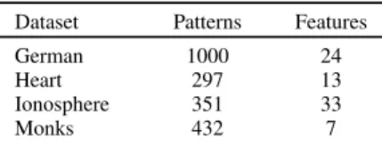
evaluation. The characteristics of the preprocessed datasets are summarized in Table I.
TABLE I: Dataset characteristics Dataset Patterns Features
German 1000 24
Heart 297 13
Ionosphere 351 33
Monks 432 7
Datasets German, Heart and Ionosphere do not have par-tition information, which is compulsory for the evaluation. Therefore we randomly split the dataset into two halves for training and testing. The partition information exists on Monks-1,-2,-3 datasets, therefore we used the original partition to perform the experiment. The numbers of training patterns in Monks-1,-2,-3 are 124, 169 and 122, respectively.
The base classifiers are LSVM models and the diversity is created by learning either from datasets using different sub-feature set or subsets of the training patterns. The ensemble accuracies are compared with the classifier using same LSVM model but trained by the entire training set.
Both NSGA-II and LSVMs we used are provided in the Shark Machine Learning Library [27]. The regularization parameterC of the LSVM algorithm is pre-tuned per dataset with k-Fold cross validation where k=3. The same optimal
TABLE II: Experiment parameters
Parameter Value
Number of ensemble member 9
Population size 500
Number of generations 500
Crossover points 2
Crossover probability 0.6
Mutation probability Lc1
*Lcdenotes the length of chromosome
training. Parameters of the NSGA-II algorithm are listed in Table II.
In the experiments, three diversity measures, i.e., CFD, DIS and HD, are used. Meanwhile, two diversity creation methods, i.e., using different features or using different training patterns are investigated. The combination of the three diversity mea-sures with two diversity creation methods result in six different setups in total, which is listed in Table III.
TABLE III: List of ensemble methods Abbreviation Diversity measure Diversity creation
CFD/SF CFD By supplying different sub features CFD/SS CFD By supplying different sub patterns DIS/SF DIS By supplying different sub features DIS/SS DIS By supplying different sub patterns HD/SF HD By supplying different sub features HD/SS HD By supplying different sub patterns
B. Experimental Results
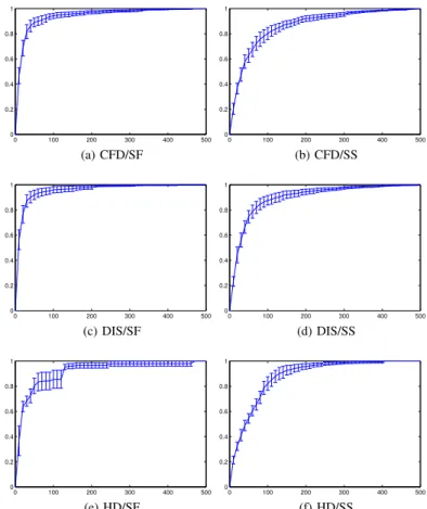
1) Convergence Analysis: We used hypervolume [28], [29]
as the performance indicator to illustrate the convergence of the NSGA-II for multi-objective ensemble generation. In this work, as both objectives are normalized between 0 and 1, the reference point is set to (0,0) in all experiments.
In the experiments, once the hypervolume stops increasing for a certain number of generations, we can conclude that the learning has converged. Note, however, that the absolute ac-curacy and diversity varies across different datasets, therefore the absolute hypervolume value cannot be used for comparing the results across different test problems. To address this issue, we linearly scaled the hypervolume from 0 to 1, so that it can indicate the degree of convergence of the learning process. The scaling is shown in (14) and the results can be found in Fig. 1.
HVi0= (HVi HV0)/(HVend HV0), (14)
where HVi denotes the hypervolume of i-th generation and
HVend denotes the result of the last generation.
Fig. 1 shows the mean and standard deviation of the hyper-volume averaged over the six test problems. From these plots, we can see that in most scenarios, learning converges within 500 generations, while different diversity measure / creation methods show different converging speeds. It is easy to see that creating diversity by supplying different features (refer to the three plots in the left panels in Fig. 1) converges faster than
0 100 200 300 400 500 0 0.2 0.4 0.6 0.8 1 (a) CFD/SF 0 100 200 300 400 500 0 0.2 0.4 0.6 0.8 1 (b) CFD/SS 0 100 200 300 400 500 0 0.2 0.4 0.6 0.8 1 (c) DIS/SF 0 100 200 300 400 500 0 0.2 0.4 0.6 0.8 1 (d) DIS/SS 0 100 200 300 400 500 0 0.2 0.4 0.6 0.8 1 (e) HD/SF 0 100 200 300 400 500 0 0.2 0.4 0.6 0.8 1 (f) HD/SS
Fig. 1: The hypervolume averaged over the six test cases for the six experimental setups.
by supplying different training patterns. This is because, in all test cases used in this work, the number of features is much smaller than that of training patterns. Therefore, searching for the optimal feature subsets takes much less time to converge than searching for the optimal training patterns. Furthermore, the convergence speed on the HD diversity measure seems slower than other diversity measures. We investigated this and found that the number of achieved Pareto solutions in this setup is significantly smaller than other diversity measures, which may make it more difficult for the MOEA to explore new solutions. This may also be the reason that caused a jump in the convergence in Fig. 1(e).
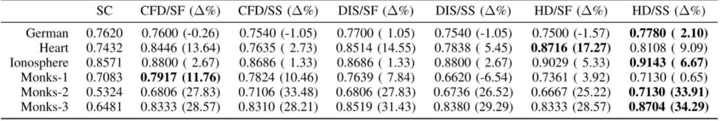
2) Classification Performance: The accuracies on the test
data of single classifier and ensemble classifiers can be found in Table IV. For better visualization, these results have also been plotted in Fig. 2.
Rows in Table IV represent the results from different datasets while columns present the test accuracies of single classifier or best accuracy of classifier ensembles found in Pareto front of the final generation. The values in brackets show the accuracy improvements compared with single classi-fiers whilst negative values mean the performance degradation. The best method is highlighted with bold font.
TABLE IV: Test accuracies of single classifier and ensemble classifiers SC CFD/SF ( %) CFD/SS ( %) DIS/SF ( %) DIS/SS ( %) HD/SF ( %) HD/SS ( %) German 0.7620 0.7600 (-0.26) 0.7540 (-1.05) 0.7700 ( 1.05) 0.7540 (-1.05) 0.7500 (-1.57) 0.7780 ( 2.10) Heart 0.7432 0.8446 (13.64) 0.7635 ( 2.73) 0.8514 (14.55) 0.7838 ( 5.45) 0.8716 (17.27) 0.8108 ( 9.09) Ionosphere 0.8571 0.8800 ( 2.67) 0.8686 ( 1.33) 0.8686 ( 1.33) 0.8800 ( 2.67) 0.9029 ( 5.33) 0.9143 ( 6.67) Monks-1 0.7083 0.7917 (11.76) 0.7824 (10.46) 0.7639 ( 7.84) 0.6620 (-6.54) 0.7361 ( 3.92) 0.7130 ( 0.65) Monks-2 0.5324 0.6806 (27.83) 0.7106 (33.48) 0.6806 (27.83) 0.6736 (26.52) 0.6667 (25.22) 0.7130 (33.91) Monks-3 0.6481 0.8333 (28.57) 0.8310 (28.21) 0.8519 (31.43) 0.8380 (29.29) 0.8333 (28.57) 0.8704 (34.29) Notations:
SC: Single Classifier. Test rate of single classifier alone. : Difference between ensemble method and single classifier.
German Heart Ionosphere Monks−1 Monks−2 Monks−3
0.5 0.55 0.6 0.65 0.7 0.75 0.8 0.85 0.9 0.95 1 Single Classifier CFD/SF CFD/SS DIS/SF DIS/SS HD/SF HD/SS
Fig. 2: Comparison of single classifier and ensemble classifiers dataset as indicated at the bottom. The seven colored bars in
each group denote the test accuracy of the single classifier and those of six ensembles created using different methods. The results show that classifier ensembles consistently improve the classification performance on four datasets, namely Heart, Ionosphere, Monk-2 and Monk-3, while mixed results have been obtained on the German and Monk-1. Meanwhile, dif-ferent diversity creation methods and measures give various accuracy improvements. This indicates that the optimal diver-sity creation method might be problem dependent.
In our experiments, 31 out of 36 ensemble setups improved classifier accuracy. In some datasets, i.e., 2 and Monks-3, classifier ensembles dramatically improved the ensembles’ accuracies by over 30% higher than the single classifiers. Only one setup, i.e., DIS/SS method on Monks-1 dataset, had significantly degraded the classification performance. We conducted some additional investigations on this dataset, and found that a few solutions that performed better than the single classifier were lost in later generations. This may indicate that this dataset is easy to overfit and additional measures for controlling overfitting are needed to ensure that good performance on the training set will also lead to good performance on the test set.
By comparing the performance over all experimental setups, we can see that combining the HD diversity measure in the input (feature) space with the use of subsets of the training patterns for creating ensemble members might be the preferred
option for creating diverse yet accurate ensembles, as it produces the best result on five of the six test cases.
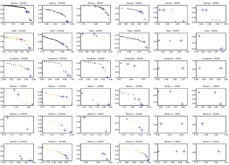
The Pareto fronts of the 36 setups are plotted in Fig. 3, where the results from the same test case are plotted in the same row and results from the same ensemble generation method are plotted in the same column. The two axes of each subplot indicate the average training accuracy and the diversity measure, respectively. Each circle denotes a generated ensem-ble on Pareto front, where black circles indicate the solutions performing worse than the single classifier and the colored circles indicate those solutions performing better. The color of these circles varies smoothly from yellow to red, where colors closer to red indicate the testing accuracy is higher. Blue crosses in the plots mark the solutions that have highest test accuracies, where the bigger the crosses are, the higher the accuracy.
Fig. 3 also shows that, not all solutions on the Pareto front outperform the single classifier. In addition, most solutions with higher accuracy on the test data are distributed near the right end of the Pareto front, i.e., the solutions have higher classification accuracy on the training data, although the best solution is not necessarily the solution having the highest training accuracy. This is quite intuitive as the solutions having very high accuracy on the training data are more likely to overfit. However, these results suggest that if we do not have additional information for selecting solutions from the Pareto front, it is still better to select ensembles having a
0.70 0.75 0.80 0.85 0.35 0.40 0.45 0.50 0.55 German − CFD/SF 0.80 0.82 0.84 0.86 0.27 0.28 0.29 0.30 0.31 German − CFD/SS 0.75 0.80 0.85 0.53 0.54 0.55 German − DIS/SF 0.83 0.84 0.85 0.86 0.87 0.28 0.29 0.30 German − DIS/SS 0.83 0.84 0.84 0.85 0.55 0.55 0.56 0.56 German − HD/SF 0.84 0.85 0.85 0.86 0.53 0.54 0.55 0.56 German − HD/SS 0.70 0.75 0.80 0.85 0.90 0.45 0.50 0.55 Heart − CFD/SF 0.70 0.80 0.90 1.00 0.45 0.50 0.55 Heart − CFD/SS 0.84 0.86 0.88 0.90 0.92 0.94 0.48 0.50 0.52 0.54 0.56 Heart − DIS/SF 0.70 0.80 0.90 1.00 0.52 0.53 0.54 0.55 Heart − DIS/SS 0.92 0.92 0.93 0.93 0.00 0.50 1.00 Heart − HD/SF 0.93 0.93 0.94 0.94 0.94 0.55 0.55 0.56 Heart − HD/SS 0.90 0.92 0.94 0.96 0.98 0.20 0.30 0.40 0.50 Ionosphere − CFD/SF 0.92 0.94 0.96 0.98 1.00 0.20 0.22 0.24 0.26 Ionosphere − CFD/SS 0.90 0.92 0.94 0.96 0.98 0.40 0.45 0.50 Ionosphere − DIS/SF 0.97 0.98 0.99 0.30 0.30 0.31 0.31 Ionosphere − DIS/SS 0.96 0.96 0.96 0.97 0.00 0.50 1.00 Ionosphere − HD/SF 0.98 0.98 0.99 0.99 0.99 0.00 0.50 1.00 Ionosphere − HD/SS 0.70 0.75 0.80 0.50 0.52 0.54 0.56 0.58 Monks−1 − CFD/SF 0.70 0.75 0.80 0.40 0.45 0.50 0.55 0.60 Monks−1 − CFD/SS 0.74 0.76 0.78 0.80 0.82 0.53 0.54 0.55 0.56 Monks−1 − DIS/SF 0.75 0.80 0.85 0.90 0.55 0.55 0.55 0.55 Monks−1 − DIS/SS 0.80 0.81 0.81 0.82 0.54 0.55 0.56 Monks−1 − HD/SF 0.81 0.82 0.83 0.84 0.85 0.53 0.54 0.55 0.56 Monks−1 − HD/SS 0.70 0.71 0.72 0.73 0.52 0.53 0.54 Monks−2 − CFD/SF 0.70 0.72 0.74 0.76 0.48 0.50 0.52 0.54 0.56 Monks−2 − CFD/SS 0.72 0.72 0.73 0.73 0.44 0.46 0.48 0.50 Monks−2 − DIS/SF 0.72 0.74 0.76 0.78 0.53 0.54 0.55 Monks−2 − DIS/SS 0.66 0.67 0.68 0.00 0.50 1.00 Monks−2 − HD/SF 0.70 0.80 0.90 1.00 0.00 0.50 1.00 Monks−2 − HD/SS 0.70 0.75 0.80 0.85 0.90 0.50 0.52 0.54 0.56 Monks−3 − CFD/SF 0.70 0.75 0.80 0.85 0.90 0.45 0.50 0.55 Monks−3 − CFD/SS 0.80 0.85 0.90 0.53 0.54 0.55 0.56 Monks−3 − DIS/SF 0.75 0.80 0.85 0.90 0.95 0.54 0.55 0.55 0.56 Monks−3 − DIS/SS 0.70 0.75 0.80 0.85 0.90 0.00 0.50 1.00 Monks−3 − HD/SF 0.70 0.80 0.90 1.00 0.00 0.50 1.00 Monks−3 − HD/SS
Fig. 3: Typical Pareto fronts achieved in the 36 different setups. higher training accuracy. Some additional experiments have
been carried out and the results indicate that selecting the top 10% on the training data overall outperform others.
V. CONCLUSION
In this paper, we proposed a method that uses the diversity measure as an explicit objective, along with the training accuracy of the ensemble as another objective. Three different diversity measures and two methods for creating ensemble diversity have been tested. Our results indicate that not all methods can reliably result in ensembles that outperform single classifiers. Overall, the diversity creation method that uses different training datasets combined with a diversity imposed on the feature space may be most likely to produce the best classification performance.
Although many good solutions could be found in the Pareto front, it is hard to figure out the solution that performs the best on the test dataset. The results suggest that although higher diversity may result in better ensemble performance, the classification accuracy of the ensemble members are still more important than the diversity of the ensemble, therefore the trade-off between these two objectives should be the biggest matter. The results of this work also show that the
best solutions that have the highest test accuracy are mostly in the top 10% of the Pareto optimal solutions having the highest training accuracy.
Future work will aim to introduce more effective constraints in evolving ensembles that can ensure that the generated ensembles are more reliable compared to a single classifier. In addition, investigations will also be made to check if addi-tional measures, e.g., the average complexity of the ensemble members, can assist the selection of solutions from the Pareto front that perform well on unseen data.
REFERENCES
[1] K. Tumer and J. Ghosh, “Error correlation and error reduction in ensemble classifiers,”Connection Science, vol. 8, no. 3-4, pp. 385–404, 1996.
[2] G. Brown, J. Wyatt, R. Harris, and X. Yao, “Diversity creation methods: A survey and categorisation,”Information Fusion, vol. 6, no. 1, pp. 5– 20, Mar. 2005.
[3] A. Krogh and J. Vedelsby, “Neural network ensembles, cross validation, and active learning,” in Advances in neural information processing systems 7, G. Tesauro, D. S. Touretzky, and T. K. Leen, Eds., 1994, pp. 231–238.
[4] D. W. Opitz and J. W. Shavlik, “Generating accurate and diverse mem-bers of a neural-network ensemble,” inAdvances in Neural Information Processing Systems. MIT Press, 1996, pp. 535–541.
[5] G. Brown, “Diversity in neural network ensembles,” Ph.D. dissertation, School of Computer Science, University of Birmingham, Jan. 2004. [6] L. Breiman, “Bagging predictors,”Machine Learning, vol. 24, no. 2, pp.
123–140, 1996.
[7] R. Meir and G. R¨atsch, “An introduction to boosting and leveraging,” in
Lecture Notes in Computer Science, S. Mendelson and A. Smola, Eds. Berlin, Heidelberg: Springer Berlin Heidelberg, 2003, pp. 118–183–183. [8] A. Chandra and X. Yao, “DIVACE: Diverse and accurate ensemble learning algorithm,” in Lecture Notes in Computer Science, Z. Yang, H. Yin, and R. Everson, Eds. Springer Berlin Heidelberg, 2004, pp. 619–625.
[9] Y. Jin and B. Sendhoff, “Pareto-based multiobjective machine learning: An overview and case studies,”IEEE Transactions on Systems, Man, and Cybernetics, Part C: Applications and Reviews, vol. 38, no. 3, pp. 397–415, 2008.
[10] Y. Liu and X. Yao, “Ensemble learning via negative correlation,”Neural Networks, vol. 12, no. 10, pp. 1399–1404, 1999.
[11] J. J. Aguilera, M. Chica, M. J. del Jesus, and F. Herrera, “Niching genetic feature selection algorithms applied to the design of fuzzy rule-based classification systems,” inFuzzy Systems Conference, 2007. FUZZ-IEEE 2007. IEEE International, Jul. 2007, pp. 1–6.
[12] Y. Jin, T. Okabe, and B. Sendhoff, “Neural network regularization and ensembling using multi-objective evolutionary algorithms,” in Evolution-ary Computation, 2004. CEC2004. Congress on, Jun. 2004, pp. 1–8 Vol.1.
[13] N. Li, Y. Yu, and Z.-H. Zhou, “Diversity regularized ensemble pruning,” in Lecture Notes in Computer Science, P. Flach, T. De Bie, and N. Cristianini, Eds. Berlin, Heidelberg: Springer Berlin Heidelberg, 2012, pp. 330–345–345.
[14] A. Chandra and X. Yao, “Ensemble learning using multi-objective evolu-tionary algorithms,”Journal of Mathematical Modelling and Algorithms, vol. 5, no. 4, pp. 417–445–445, 2006.
[15] N. Ghoggali, F. Melgani, and Y. Bazi, “A multiobjective genetic SVM approach for classification problems with limited training samples,”
IEEE Transactions on Geoscience and Remote Sensing, vol. 47, no. 6, pp. 1707–1718, 2009.
[16] U. Bhowan, M. Johnston, M. Zhang, and X. Yao, “Evolving diverse ensembles using genetic programming for classification with unbalanced
data,”IEEE Transactions on Evolutionary Computation, vol. 17, no. 3, pp. 368–386, 2013.
[17] C. Smith and Y. Jin, “Evolutionary multi-objective generation of recur-rent neural network ensembles for time series prediction,” Neurocom-puting, vol. 143, no. 0, pp. 302–311, 2014.
[18] K. P. Bennett and C. Campbell, “Support vector machines: hype or hallelujah?”ACM SIGKDD Explorations Newsletter, vol. 2, no. 2, pp. 1–13, 2000.
[19] C. J. C. Burges, “A tutorial on support vector machines for pattern recognition,”Data Mining and Knowledge Discovery, vol. 2, no. 2, pp. 121–167, Jan. 1998.
[20] E. K. Tang, P. N. Suganthan, and X. Yao, “An analysis of diversity measures,”Machine Learning, vol. 65, no. 1, pp. 247–271–271, 2006. [21] L. Kuncheva and C. Whitaker, “Measures of diversity in classifier
ensembles and their relationship with the ensemble accuracy,”Machine Learning, vol. 51, no. 2, pp. 181–207, 2003.
[22] T. Windeatt, “Diversity measures for multiple classifier system analysis and design,”Information Fusion, vol. 6, no. 1, pp. 21–36, Mar. 2005. [23] K. Trawi´nski, O. Cord´on, and A. Quirin, “A study on the use of
multiobjective genetic algorithms for classifier selection in FURIA-based fuzzy multiclassifiers,” International Journal of Computational Intelligence Systems, vol. 5, no. 2, pp. 231–253, 2012.
[24] K. Trawi´nski, O. Cord´on, A. Quirin, and L. S´anchez, “Multiobjective genetic classifier selection for random oracles fuzzy rule-based classifier ensembles: How beneficial is the additional diversity?” Knowledge-Based Systems, vol. 54, no. 0, pp. 3–21, 2013.
[25] K. Deb, A. Pratap, S. Agarwal, and T. Meyarivan, “A fast and elitist multiobjective genetic algorithm: NSGA-II,” IEEE Transactions on Evolutionary Computation, vol. 6, no. 2, pp. 182–197, 2002.
[26] K. Bache and M. Lichman, “UCI machine learning repository,” 2013. [Online]. Available: http://archive.ics.uci.edu/ml
[27] C. Igel, V. Heidrich-Meisner, and T. Glasmachers, “Shark,”Journal of Machine Learning Research, vol. 9, pp. 993–996, 2008.
[28] E. Zitzler and L. Thiele, “Multiobjective optimization using evolutionary algorithms - A comparative case study,” inLecture Notes in Computer Science, A. Eiben, T. B¨ack, M. Schoenauer, and H.-P. Schwefel, Eds. Berlin/Heidelberg: Springer Berlin Heidelberg, 1998, pp. 292–301–301. [29] E. Zitzler, Evolutionary algorithms for multiobjective optimization: