Dynamic multi-objective optimization: a two archive strategy

(1)

DYNAMIC MULTI-OBJECTIVE OPTIMIZATION:

A TWO ARCHIVE STRATEGY

by

Renzhi Chen

A thesis submitted to

The University of Birmingham

for the degree of

DOCTOR OF PHILOSOPHY

School of Computer Science

College of Engineering and Physical Sciences

The University of Birmingham

(2)

University of Birmingham Research Archive

e-theses repository

This unpublished thesis/dissertation is copyright of the author and/or third parties. The intellectual property rights of the author or third parties in respect of this work are as defined by The Copyright Designs and Patents Act 1988 or as modified by any successor legislation.

Any use made of information contained in this thesis/dissertation must be in accordance with that legislation and must be properly acknowledged. Further distribution or reproduction in any format is prohibited without the permission of the copyright holder.

(3)

(4)

ABSTRACT

Existing studies on dynamic multi-objective optimization mainly focus on dynamic prob-lems with time-dependent objective functions. Few works have put efforts on dynamic problems with a changing number of objectives, or dynamic problems with time-dependent constraints. When problems have time-dependent objective functions, the shape or posi-tion of the Pareto-optimal front/set may change over time. However, when dealing with problems with a changing objective number or time-dependent constraints, the challenges are different. Changing number of objectives leads to the expansion or contraction of the dimensions of the Pareto-optimal front/set manifold, while time-dependent constraints may change the shape of feasible regions over time. The existing dynamic handling techniques can hardly handle the changing number of objectives. The state-of-arts in constraints handling techniques are incapable of tackling problems with time-dependent constraints. In this thesis, we present our attempts toward tackling 1) the dynamic multi-objective optimizing problems with a changing number of multi-objectives and 2) multi-multi-objective optimizing problems with time-dependent constraints. Two-archive Evolutionary Algo-rithms are proposed. Comprehensive experiments are conducted on various benchmark problems for both types of dynamics. Empirical results fully demonstrate the effectiveness of our proposed algorithms.

(5)

(6)

ACKNOWLEDGEMENT

I would like to express my deepest gratitude to my supervisor Prof. Xin Yao, for his academic support in the past four years. His rich knowledge in the field of evolutionary algorithms and insightful comments in every meeting have deepened my understanding in this research area and helped me improve my research. I could not have imagined having a better supervisor than him for my PhD life.

I am also grateful to Dr. Ke Li. He is a very good mentor. He gave me many support and guidance on the projects in the past one year.

I thank all the members of my RSMG group: Prof. John Barnden, Prof. John Bullinaria, and Dr. Rami Bahsoon. They have provided helpful suggestions in my every RSMG report. Their good questions in the RSMG meetings inspires me to improve my research thereafter.

Last but not least, my deepest thanks go to my families. They have continuously given my mental support and encouragement whenever I encounter difficulties in life and work.

(7)

(8)

LIST OF FIGURES

2.1 Importance of feasibility maintenance . . . 22

2.2 Framework of dynamic handling technique . . . 27

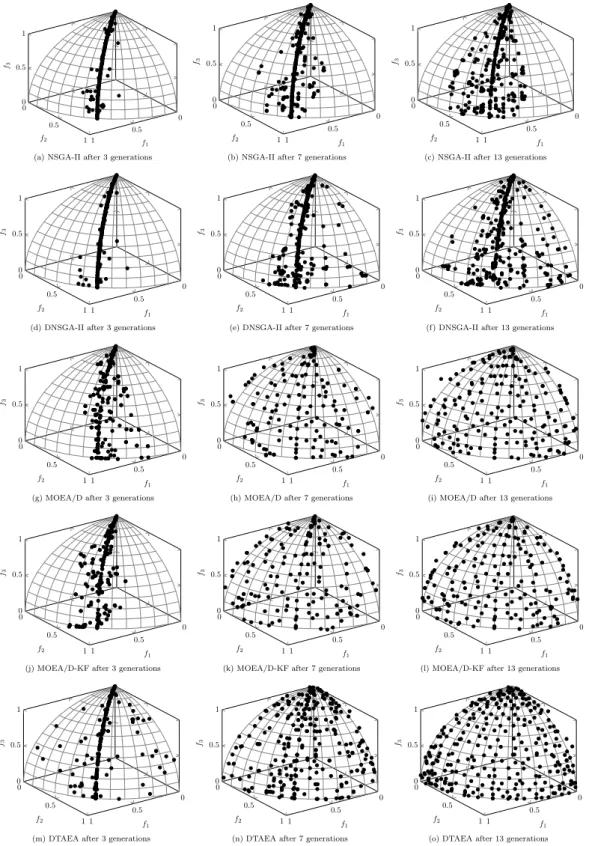
3.1 Comparison of population distributions when increasing the number of ob-jectives. . . 37

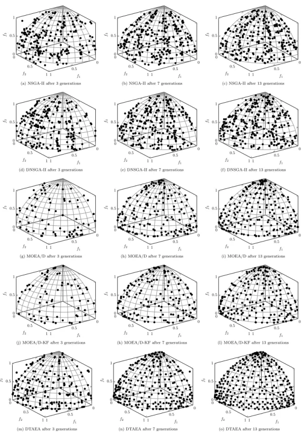
3.2 Comparison of population distributions when decreasing the number of objectives. . . 39

3.3 Flow chart of DTAEA. . . 41

3.4 An example of the CA’s update mechanism. Note that xi _{is denoted as its} index ifor short. . . 45

3.5 An example of the DA’s update mechanism. Note that xi _{is denoted as its} index ifor short. . . 48

3.6 IGD trajectories across the whole evolution process(F1,F2). . . 60

3.9 The rank of IGD obtained by different algorithms at each time step(F1,F2). 63 3.10 The rank of IGD obtained by different algorithms at each time step(F3,F4). 64 3.11 The rank of IGD obtained by different algorithms at each time step(F5,F6). 65 3.12 Variation of the population distribution when increasing the number of objectives from 2 to 3. . . 68

3.13 Variation of the population distribution when decreasing the number of objectives from 4 to 3. . . 69

(13)

3.14 Proportion of the second mating parent selected from the CA and DA

respectively. . . 70

3.15 IGD trajectories across the whole evolution process(m0(t))(F1,F2). . . 76

3.18 The rank of IGD obtained by different algorithms at each time step(m0(t)) (F1,F2). . . 79

3.19 The rank of IGD obtained by different algorithms at each time step(m0(t))(F3,F4). 80 3.20 The rank of IGD obtained by different algorithms at each time step(m0(t))(F5,F6). 81 3.21 Comparison of population distributions when decreasing the number of objectives with mixed variables. . . 87

3.22 Flow chart of solving many-objectives in a changing number of objectives way. . . 88

3.23 IGD for DTLZ2(two-obj to 15-obj) . . . 90

3.24 Flowchart of Rational Unified Process. . . 93

4.1 Examples of problems with partitioned objective space . . . 101

4.2 Examples for problems with dynamic constraints . . . 102

4.3 CV for DC2-DTLZ2 . . . 104

4.4 Illustration of C-DTLZ Series in 2D . . . 112

4.5 Illustration of DC1-DTLZ1 and DC1-DTLZ3 in 2D . . . 113

4.7 Variation of CV(x) with respect to g(x) . . . 114

4.9 Scatter plots of the population obtained by C-TAEA and the peer algo-rithms on C1-DTLZ3 (median IGD value). . . 121

4.10 Scatter plots of the population obtained by C-TAEA and the peer algo-rithms on C2-DTLZ2 (median IGD value). . . 122

(14)

4.11 Comparison of the solutions finally obtained in CA and DA on C2-DTLZ2

(median IGD value). . . 122

4.12 Scatter plots of the population obtained by C-TAEA and the peer algo-rithms on DC1-DTLZ1 (median IGD value). . . 124

4.18 Layout of the anytown WDN. . . 132

4.19 Box plots of HV obtained by different algorithms. . . 136

4.20 Comparison of population distributions for Type-A . . . 140

4.21 Comparison of population distributions for Type-B. . . 140

(15)

(16)

LIST OF TABLES

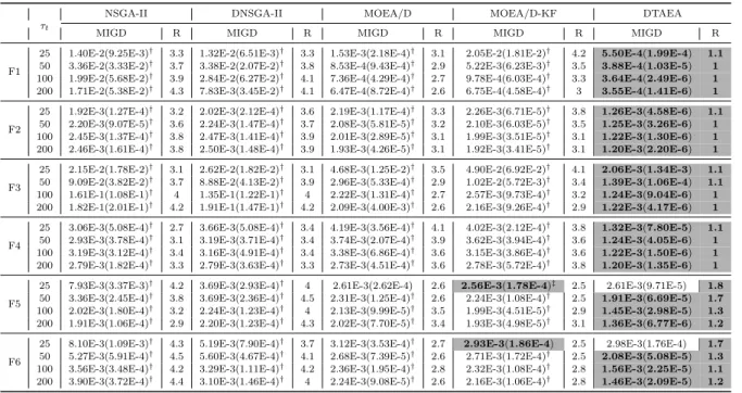
3.1 Mathematical Definitions of Dynamic Multi-Objective Benchmark Problems 51 3.2 Performance Comparisons of DTAEA and the Other Algorithms on MIGD

Metric . . . 59

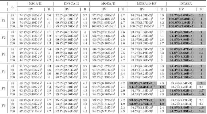
3.3 Performance Comparisons of DTAEA and the Other Algorithms on MHV Metric . . . 66

3.4 Performance Comparisons of DTAEA and its Three Variants on MIGD Metric . . . 72

3.5 Performance Comparisons of DTAEA and its Three Variants on MHV Metric 73 3.6 Average ranking for different changing frequency . . . 73

3.7 Performance Comparisons of DTAEA and its Three Variants on MIGD Metric (m0(t)) . . . 75

3.8 Performance Comparisons of DTAEA and its Three Variants on MHV Metric(m0(t)) . . . 82

3.9 Performance Comparisons of DTAEA dealing problem with 3 types of non-partitioned variables on IGD Metric(m0(t)) . . . 86

3.10 Result of IGD solving 15-objective DTLZ series . . . 91

3.11 Median HV and iqr on the scheduling problem on RUP . . . 95

3.12 Skill table and the per hour salary for 10 employees . . . 95

3.13 Workloads for the Scheduling Problem . . . 96

4.1 Mathematical Definitions of DTLZ Test Problems . . . 110

(17)

4.3 Comparison results on IGD metric (median and IQR) for C-TAEA and the other peer algorithms on C-DTLZ benchmark suite . . . 120 4.4 Comparison results on HV metric (median and IQR) for C-TAEA and the

other peer algorithms on C-DTLZ benchmark suite . . . 120 4.5 Number of runs when finding feasible solutions. . . 125 4.6 Comparison results on IGD metric (median and IQR) for C-TAEA and the

other peer algorithms on DC-DTLZ benchmark suite . . . 128 4.7 Comparison results on HV metric (median and IQR) for C-TAEA and the

other peer algorithms on DC-DTLZ benchmark suite . . . 129 4.8 Comparison results on IGD metric (median and IQR) for C-TAEA and the

other peer algorithms on Dynamic C-DTLZ benchmark suite . . . 130 4.9 Problems with six types of changes . . . 138 4.10 Mathematical Definitions of Dynamic Multi-Objective Benchmark Problems142 4.11 Performance Comparisons of C-DTAEA and the Other Algorithms on MIGD

(18)

NOMENCLATURE

Acronyms

MOP(s) Multi-objective optimization problem(s) DMO Dynamic multi-objective optimization DM(s) Decision maker(s)

PS Pareto-optimal set PF Pareto-optimal front EA(s) Evolutionary Algorithm(s)

MOEA(s) Multi-objective evolutionary algorithm(s) CA Convergence archive

DA Diversity archive

CMOEA(s) Constrained multi-objective evolutionary algorithms CMOP(s) Constrained multi-objective optimization problem(s) DMOPs Dynamic multi-objective optimization problems

DCMOP(s) Dynamic constrained multi-objective optimization problem(s) RUP Rational Unified Process

QoS Quality of service CV Constraint violation

CDR Constrained dominance relation WDN Water distribution network problems IQR interquartile range

GD Generational Distance

IGD Inverted Generational Distance MIGD Mean Inverted Generational Distance

HV Hypervolume

MHV Mean Hypervolume

(19)

Algorithms

NSGA-II Non-dominated sorting genetic algorithm II SPEA2 Improved strength Pareto EA

IBEA indicator-based evolutionary algorithm MOEA/D Multi-objective EA based on decomposition TAEA Two-archive evolutionary algorithms

DTAEA Dynamic two-archive evolutionary algorithm C-TAEA Constrained two-archive EA

C-DTAEA Constrained dynamic two-archive EA

DNSGA-II Dynamic non-dominated sorting genetic algorithm II

MOEA/D-KF Multi-objective EA based on decomposition with Kalman Filter predictor C-MOEA/D Constrained multi-objective EA based on decomposition

C-NSGA-III Constrained non-dominated sorting genetic algorithm III

C-MOEA/DD Constrained MOEA based on Pareto dominance and Decomposition I-DBEA Independent distances based EA

CMOEA Algorithm for CMOPs proposed by Woldesenbet et al. CMOEA/D constrained multi-objective EA based on decomposition

(20)

CHAPTER 1

INTRODUCTION

Multi-objective optimization problems (MOPs) consider optimizing more than one con-flicting objective simultaneously. MOPs arise in many engineering applications when optimal decisions need to be taken in the presence of two or more conflicting objectives. For example, in motor design [1], maximizing the engine performance and minimizing the pollution emission are two typical conflicting objectives in motor design. When optimizing the aerodynamics performance of a high-speed train head [2], minimizing the drag force and the lift force are conflicting with each other. In multi-objective optimization, there does not exist a global optimum, which optimizes all objectives. Instead, decision makers (DMs) are often interested in a set of trade-off solutions which scarifies one objective for the other. The concept of Pareto dominance is introduced to determine which solution is better in the comparison when considering multiple conflicting objectives. Specifically, solution A is said to dominate a solution B if and only if 1) solution A is not worse than solution B in all objectives and 2) solution A is better than solution B in at least one objective. A solution is called Pareto-optimal in case that there does not exist any other solution dominate it. The set of Pareto-optimal solutions in the decision space is called the Pareto-optimal set (PS), and its corresponding mapping in the objective space form the Pareto-optimal front (PF).

Evolutionary Algorithm (EA), inspired by biological evolution, has been recognized as a popular approach for multi-objective optimization. EAs maintain a set of solutions, also

(21)

known as a population, during the optimization process. In each iteration, offspring solu-tions are reproduced from current solusolu-tions through the crossover and mutation. These offspring solutions have possibilities to replace solutions in the current population dur-ing the selection process. EA has been widely accepted for solvdur-ing MOPs because of its population-based nature which enables the approximation of a set of non-dominated solutions in a single simulation run. Generally speaking, there are three basic goals in evo-lutionary multi-objective optimization: 1) approximating the PF as close as possible (this is known as convergence), 2) making sure that the population distribution is as uniform as possible and 3) making sure that the population covers the whole PF as much as pos-sible. In particular, the latter two are also known as diversity. In the past three decades and beyond, many efforts have been devoted to the development of multi-objective EAs for achieving the balance between convergence and diversity. Many multi-objective evo-lutionary algorithms (MOEAs) have been proposed over the past three decades, such as non-dominated sorting genetic algorithm II (NSGA-II) [3], indicator-based EA (IBEA) [4], multi-objective EA based on decomposition (MOEA/D) [5]. Praditwong and Yao pro-posed to use a two-archive mechanism [6, 7]. In particular, as convergence and diversity are two separate goals in EMO, their basic idea is to use two complementary populations to achieve the convergence and the diversity separately. As the first attempt, this two-archive mechanism has been proved to work on some benchmark problems and it also forms the algorithmic foundation of the methodologies developed in this thesis.

Furthermore, constrained optimization is ubiquitous in the real world, whereas studies on constrained multi-objective optimization (CMO) have been surprisingly lukewarm in the literature. Most, if not all, existing constraint handling techniques simply borrow ideas from single-objective optimization. In particular, they mainly aim at pushing the population toward the feasible region as much as possible before considering the balance between convergence and diversity within the feasible region. Furthermore, few works have pay attention to the importance of infeasible solutions. Most, if not all, existing constraint handling techniques tend to push a population toward the feasible region as

(22)

much as possible before considering the balance between convergence and diversity within the feasible region. Few works have pay attention to the value of infeasible solutions. However, in some complex situations, algorithms cannot handle the constrained problems without exploring the infeasible region or maintaining some infeasible solutions. One example can be found in the scenario where two feasible regions are separated by an infeasible barrier. It is hard to push a solution from one feasible region to the other without entering the infeasible barrier.

In addition, it is not uncommon that real-world optimization scenarios are fully of dy-namics or uncertainties. In recent years, dynamic multi-objective optimization (DMO) has become increasingly popular in the EMO community. Generally speaking, a DMO prob-lem (DMOP) can involve various types of dynamic characteristics, e.g. time-dependent objective and/or constraint functions, and a changing dimensionality (in terms of the number of variables or objectives). Thus, DMOP is intrinsically more challenging due to the existence of dynamics. Due to the population-based property and its self-adaptation, the EA has been widely used to solve DMOPs. However, the current studies on DMO mainly focus on problems whose function formulations will change over time, whereas very limited studies have been on considering the change of dimensionality (e.g. the number of objectives and/or constraints change over time). Note that this sort of dynamic problems are not uncommon in the real world where we will delineate in the later chapters. The challenges for MOPs with changing number of objectives are different from the MOPs with time-dependent objective functions. When objectives are added or removed during the search process, instead of changing the position or the shape of the original PS/PF, the dimension of PS/PF manifold will expand or contract. Besides the changing number of objectives, the constraints for MOPs may change during the optimization process as well. We name problems with dynamic constraints as dynamic constrained multi-objective op-timization problems (DCMOPs). Dynamic constraints can be classified into many types. In this thesis, we only discuss problems with time-dependent constraints, which are not fully studied. Current dynamic handling techniques cannot handle this type of problems

(23)

as the challenges for DCMOPs come from two aspects: 1) finding converged and well-diversified feasible solutions before changes, and 2) tracking the moving feasible region after changes.

the following paragraphs, we first describe the motivations that lead to the research conducted in this thesis. Afterwards, we outline the main contributions of this thesis.

1.1

Motivations

EAs have been widely used for solving MOPs since the 1990s. Whereas many real-world scenarios consider problems in a uncertain environment, e.g. the objective and/or the constraint functions can change over time, these changes have an in-negligible impact on the process of optimization: the time-dependent objective functions may lead to a moving PS/PF; adding or removing objectives may cause the expanding or contracting of the dimension of PS/PF manifold; changing constraints may cause a changing feasible region. These challenges bring about the emerging interests for the research for DMO. In the past decade, many efforts have been devoted to develop various methods for handling problems with a time-dependent objective functions [8, 9]. Whereas, another dynamic scenario, i.e. problems with a changing number of objectives which is not uncommon in the real-world scenarios, has rarely been studied in the literature. In particular, we will describe some scenarios that lead to such dynamic characteristics.

• The number of objective functions changes naturally as a requirement from the real-life optimization scenarios. For example, in the model of Rational Unified Pro-cess (RUP) in software project scheduling problem, the number of quality function changes as the project steps into different phases, resulting in a changing number of objectives. Similar situations also happen in scheduling resources under a cloud computing environment, where the quality of service (QoS) for a particular user is an objective in the optimization process. The number objectives for QoS varies

(24)

• The number of objective functions possibly changed as the expectation of DMs. In business management, there exist many operational aspirations/objectives. The performance objectives of operations management include quality, speed, flexibility, dependability and cost [10]. The optimization process tries to find trade-offs among these objectives. As a DM, (s)he can choose to optimize different objectives given the requirements at a particular operational stage.

• Modelling real-world optimization scenarios is very challenging in some cases. It is difficult to request a thoroughly considered optimization problem before the opti-mization process starts. Allowing the model builder to revise the model and change the number of objectives during the optimization can reduce the difficulty of mod-elling. The model builder can bear less pressure in the modelling as they still have chances to change afterwards during the optimization process.

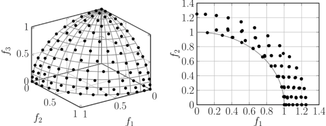
Different from the challenges from the time-dependent objective functions, the DMOPs with a changing number of objectives usually cause the expansion or contraction of the dimension of the PS/PF manifold. Generally speaking, there are two key characteristics of DMOPs with a changing number of objectives. First, the Pareto-optimal solutions before the change will still be Pareto optimal after the increase of the number of objec-tives. Second, as the dimension of the PS/PF manifold will be changed after changing the number of objectives, the Pareto-optimal solutions before the change will be either crowded in a small area on the PF after the change, or partly drifted away from the PF after the change. These characteristics will be further discussed in the Section 3.1. Algorithms designed for the DMOPs with time-dependent objective functions have diffi-culties to handle this problem. Prediction-based methods such as PPS [8] aim to track the centre of the PF. By relocating solutions according to the predicted centre, these methods can successfully track the moving of PF. However, when the dimension of PF manifold expands or contracts, rather than moving, these relocating methods fail. Intro-ducing diversified solutions such as DNSGA-II [9] also cannot tackle the challenges. The reasons are as follow: 1) for the situation of increasing number of objectives, a few newly

(25)

introduced solutions are easily dominated by current solutions, as current solutions are all close to the PF. Adding more solutions can solve the problem. However, it will also ruin the convergence of the population, as too many random solutions are in the population. 2) For the situation of decreasing number of objectives, the challenge for this situation is that many solutions are drifted away from the PF, whereas the newly introduced solutions cannot help push the drifted solutions back to the PF. The historical information only works well on periodic changes.

Besides of the DMOPs, many techniques have been proposed to handle the CMOPs. One of the major issues of solving CMOPs is how to deal with the infeasible solutions throughout the search process. Algorithms designed for CMOPs have constraints han-dling techniques, which push solutions from infeasible region to the feasible region. Most of the constraints handling techniques rely on an certain “indicator” which measures the “quality” of a solution. For example 1) feasible solutions are better than infeasible ones, 2) solutions closer to the feasible region are preferable than those far apart from the feasible boundary. It is worth to mention that constraint violation (CV) is one of the most pop-ular indicators developed along this line. Many MOEA can successfully handle CMOPs when using the CV based constrained dominance relation (CDR), such as CNSGA-II, CNSGA-III and CMOEA/D. However, these algorithms overemphasize the importance of feasibility. This can lead to an ineffective search when the algorithms encounter com-plex constraints. First, the optimization process can be misled by the local optima of a particular indicator. For example, a solution with a larger CV can be much closer to the feasible region than a solution with a smaller CV in a complex situation. Second, algorithms may fail to locate all feasible regions in case they are disparately distributed in the search space. Take a situation of two separated feasible regions as an example. When one feasible region is explored first, solutions will quickly gather in this region as algorithms prefer feasible solutions than infeasible ones. However, it is very difficult for solutions to go through the infeasible region from this feasible region to the other feasible region.

(26)

It is inarguable that problems become even more challenging when having a time-varying constraint. To the best of my knowledge, no algorithm has been developed for DCMOPs. Handling DCMOPs with algorithms designed for CMOPs has drawbacks. First, newly generated feasible solution will replace infeasible solution which closes to the PF but becomes infeasible after changes. This may ruins the convergence of the population, especially in a frequently changing situation. Second, the changing constraints may make the constraints handling techniques fail. The algorithms may always track the moving local optimal for a particular indicator, e.g. CV, rather than push solutions towards the PF. It is even more challenging to combine all the dynamics mentioned above. In the situation of DMOPs with both a changing number of objectives and dynamic constraints, there are much more issues need to be considered.

Overall, the DMOPs with a changing number of objectives are not uncommon, whereas the current algorithms designed for the DMOPs with time-dependent objective functions cannot handle this. Besides, there are some drawbacks for the existing algorithms for CMOPs. In addition, no research have been done for MOPs with dynamic constraints by the researchers. These problems challenges the current algorithms for static constraints.

The DMOP with a changing number of objectives together with dynamic constraints is a more complicated situation to deal with. All these suggest that we develop algorithms to tackle these problems.

1.2

Contributions

The main contributions of the thesis are outlined as follows:

• We have conducted an analysis and discussion on the challenges of DMOPs with a changing number of objectives in Section 3.1. The main challenges for DMOPs with a changing number of objectives are: 1) increasing number of objectives im-pacts slightly for the convergence of the population, but it ruins the diversity of the population. 2) decreasing number of objectives drags some solutions into the

(27)

search space, but the rest of the solutions stay close to the PF. We have significantly enhanced the two-archive evolutionary algorithm, by adapting to the DMOPs with a changing number of objectives. The algorithm, named dynamic two-archive evo-lutionary algorithm (DTAEA), are designed according to the characteristics for the DMOPs with a changing number of objectives. Similar to other two-archive al-gorithms, the CA in DTAEA prefer solutions close to the PF, while the diversity archive maintains solutions which can enhance the diversity. Unlike other two-archive algorithms, DTAEA stresses that the DA is a complement to the CA. Based on this and the characteristics of DMOPs with a changing number of objectives, the update, selection and reproduction mechanisms are designed. The two main charac-teristics are: 1) the PS/PF before the change is a subset of the one after increasing the number of objectives, and vice versa; and 2) instead of changing the position or the shape of the original PS/PF, increasing or decreasing the number of objectives usually results in the expansion and contraction of the dimension of the PS/PF manifold. In the experiments, DTAEA shows better results in most of the cases compared with other four state-of-art algorithms designed for DMOPs or MOPs. Moreover, several research questions have been raised and discussed, which include further understanding of how the component contributes to DTAEA, in what con-ditions DTAEA may fail. In addition, a new approach solving the many-objective optimization problem is proposed.

• We have proposed a two-archive EA, denoted as C-TAEA, to solve constrained MOPs. We discuss the challenges for the existing algorithms to solve constrained MOPs. Although current algorithms for constraints handling perform well in many cases, they cannot handle complicated searching situations. Based on the same idea of DTAEA, the main characteristics of C-TAEA are 1) the CA prefers well-converged and feasible solutions, which provides selection pressures toward the PF. 2)the DA explores the areas that have not been or will not be exploited by the CA, including areas in which CA cannot find well-converged solutions in infeasible

(28)

areas. Due to the lack of test problems for scalable constrained MOPs, we proposed our own test problems, which is denoted as DC-DTLZ series. In the experiments, C-TAEA shows better results in many cases, including the test problems of the constrained DTLZ (C-DTLZ) series [11] and self-designed DC-DTLZ series. Then we adapt the C-TAEA for the MOPs with dynamic constraints. By adding the reconstructing mechanism and adapting the mating mechanism for the dynamic situation, the C-TAEA can handle the dynamic constraints. We test the algorithm on the test problems which adapted from C-DTLZ and DC-DTLZ series. The dynamic constraints includes only time-dependent constraints functions. A changing number of constraints is not considered. The C-TAEA performs well on all the situations while other algorithms fail.

• We have adapted the C-TAEA to the water distribution network problems (WDN). The WDN is a real-life case study with four objectives and two time-dependent constraints. We use C-TAEA to solve one of the most difficult test problems for WDN, known as anytown WDN. The performance of C-TAEA is better than other five algorithms.

• We have enhanced and combined the C-TAEA and DTAEA for the DMOPs with a changing number of objectives and dynamic constraints. We have conducted a analysis and discussion on the DMOPs with a changing number of objectives. The algorithm, named constrained dynamic two-archive evolutionary algorithm (C-DTAEA), is proposed. C-DTAEA is mainly designed to handle a changing number of objectives as well as dynamic constraints. Although these scenarios are different, thebasic requirement for the algorithms is: the algorithms should have strong ability to explore the search space. While the CA behaves similar to all other algorithms, the DA in C-DTAEA is the key role. The DA will maintain non-dominated but infeasible solutions, as well as dominated solution, but helpful to the diversity. On the proposed test problems as well as the the dynamic C-DTLZ series adapted from

(29)

C-DTLZ series [11], C-DTAEA achieves a excellent results: C-DTAEA is better than other five algorithms on 15 out of 16 case.

1.3

Publications

• Renzhi Chen, Peter R. Lewis, Xin Yao: Temperature management for heterogeneous multi-core FPGAs using adaptive evolutionary multi-objective approaches. ICES 2014: 101-108

• Renzhi Chen, Ke Li, Xin Yao: Dynamic Multi-objectives Optimization With a Changing Number of Objectives. IEEE Trans. Evolutionary Computation 22(1): 157-171 (2018)

• Ke Li, Renzhi Chen, Guangtao Fu and Xin Yao: Two-Archive Evolutionary Algo-rithm for Constrained Multi-Objective Optimization. IEEE Trans. on Evolutionary Computation: online on 19/7/2018.

• Ke Li, Renzhi Chen, Geyong Min and Xin Yao: Integration of Preferences in De-composition Multi-Objective Optimization. IEEE Trans. on Cybernetics: published online on 20/8/2018.

(30)

CHAPTER 2

BACKGROUND

This chapter will at first provide some basic knowledge useful in this thesis. Afterwards, a literature review will lead you to overview some important developments in dynamic multi-objective optimization and constrained multi-objective optimization. This chap-ter is organised as follow. Section 2.1 describes the basic concepts for multi-objective optimisation and dynamic multi-objective optimisation. Section 2.2 introduces the evo-lutionary multi-objective optimization. Section 2.3 provides a review of evolutionary constrained multi-objective optimization. A brief introduction for evolutionary dynamic multi-objective optimization is given in Section 2.4.

2.1

Basic Concepts

This section includes the basic concepts for MOPs (Section 2.1.1), and DMOPs (Section 2.1.2).

(31)

2.1.1

Multi-objective Optimization

The multi-objective optimization problem (MOP) considered in this thesis is mathemat-ically defined as:

minimize F(x) = (f₁(x),· · ·,fm(x))T

subject to G(x)≤0

H(x) = 0

x∈Ω

(2.1)

where x is a vector of n decision variables: x = (x1,x2, ...,xn)T,x ∈ Ω. Ω ⊆ Rn is the

decision (variable) space.

The constrained functions includepinequality constraintsG(x) = (G1(x),G2(x), ...,Gp(x))T

andqequality constraintsH(x) = (H1(x),H2(x), ...,Hq(x))T. Solutionxis calledfeasible solution if it satisfies all the constraints functions. A solution violating any constraints is calledinfeasible solution.

Involving more than one objective function to be optimized simultaneously, most often, no single solution exists, which optimizes every objective for a non-trivial multi-objective optimization problem. Instead of a single solution, a set of solutions, denoted as Pareto-optimal solutions, is used to reflect the preference of the problem. Pareto dominance is used to define this preference. A solution x1 _∈_{Ω is said to be} _{Pareto dominate} _solution

x2 _∈_{Ω, denoted by} _x1 _≺_x2_{, if and only if the following condition is satisfied:}

∀i∈ {1, 2, ...,m},fi(x1)≤fi(x2) ∧ ∃j ∈ {1, 2, ...,m},fj(x1)< fj(x2)

A solution x is said to be Pareto optimal, if and only if _@x∗ _∈ _Ω,_x∗ _≺ _x_{. The set}

of Pareto-optimal solutions in the decision space is called as Pareto-optimal Set (PS),

P S ={x∈Ω|_@x∗ _∈_Ω,_x∗ _≺_x_}_{. The corresponding set of vectors in the objective space}

(32)

2.1.2

Dynamic Multi-objective Optimization

There are various types of dynamic characteristics that can result in different mathemati-cal definitions. Farina et al. [12] only includes problems with changing objective functions in their definition. Raquel et al. [13] adapt the definition by Nguyen et al. [14], which includes time-linkage dynamic problems. Huang et al. [15] propose their definition which includes both changing the number of objective functions and changing the number of constraints. The focus of this thesis mainly stays on the continuous DMOPs defined as follows: minimize F(x,t) = (f1(x,t),· · · ,fm(t)(x,t))T subject to G(x,t) = (G1(x,t),G2(x,t), ...,Gp(t)(x),t)T ≤0 H(x,t) = (H1(x,t),H2(x,t), ...,Hq(t)(x,t))T = 0 x∈Ωt t∈T (2.2)

T ={t1,t2,· · · ,tmax} ⊆ N is the set of time steps of the optimization process. ti is the

i-th time step in the optimization process. Ωt ⊆Rn(t) is the decision (variable) space at time stept, x= (x1,· · · ,xn(t))T ∈Ωt is a candidate solution. F: Ω →Rm(t) constitutes ofm(t) real-valued objective functions and_Rm(t) _{is called the objective space at time step}

t. The constrained functions includesp(t) inequality constraintsG(x,t) andq(t) equality constraintsH(x,t). n(t),m(t),p(t) and q(t) are functions oft.

At time step t, x1 _{is said to} _{Pareto dominate} _x2_{, denoted as} _x1 _≺

t x2, if and only if

the following condition is satisfied:

∀i∈ {1,· · · ,m(t)},fi(x1,t)≤fi(x2,t)∧ ∃j ∈ {1,· · · ,m(t)},fj(x1,t)< fj(x2,t)

At time step t, x∈ Ω is said to be Pareto-optimal, if and only if _@x∗ _∈_Ω,_x∗ _≺

t x. The

set of all Pareto-optimal solutions is called the t-th PS (denoted as PSt), P St = {x ∈

(33)

the t-th PF (denoted as PFt), P Ft={F(x,t)|x∈P St}.

2.2

Basic knowledge of Evolutionary Multi-objective

Optimization

This section provides some basic knowledge related to the use of EAs for solving MOPs, as known as evolutionary multi-objective optimization. It includes an introduction of basic elements of an MOEA, some existing develops in evolutionary multi-objective optimiza-tion, indicators for performance assessment and benchmark problems.

2.2.1

Introduction

By mimicking the process of natural evolution, EAs become one of the most important optimization methods. EAs are found to be efficient when dealing with MOPs. EAs have been used to solve MOPs in many areas including chemistry [16], physic [17], engineering [18] and etc. This is because of its population-based characteristic which enables EA to approximate a set of trade-off alternatives in a single run. In multi-objective optimization, achieving a balance between convergence and diversity is essential, i.e. finding a set of solutions not only approximate the PF as close as possible (as known as convergence) but also have a well distribution (as known as diversity).

Generally speaking, a basic MOEA includes the following major steps.

• Step 1 Generate the initial population of solutions. (denoted as population initial-ization)

• Step 2 Evaluate the fitness of each solutions in the population.

• Step 3 Repeat the following regeneration steps until termination:

– Step 3.1 Select solutions for reproduction. (denoted as mating selection)

(34)

– Step 3.3 Evaluate the fitness of each solutions in the offspring.

– Step 3.4 Combine the parent and the offspring populations; and select the fittest solutions to form the next parents. (denoted as environmental selection)

In the following paragraphs, I will further explain some more details of the above men-tioned steps.

Population Initialization

Population initialization generates solutions as the initial population for EAs, which is an important part of EAs. The initial population of a evolutionary algorithm can affect the convergence speed and also the quality of the final result [19]. Without any prior knowledge from DMs, random sampling is the most common method to generate candidate solutions. Here, some popular sampling methods are outlined as follows.

• The default uniform pseudo-random number generator are commonly applied in most of the algorithms. This generator is usually applied in the complier’s standard library, such as therand() in the C library and RANDOM class in the Java library.

• Latin Hypercube Sampling (LHS) [20] can reduce the variance in the Monte Carlo estimate of the integrand. The range of the variables is divided into intervals of equal probability. The variables are selected randomly according to the probability density in the interval. Then random pairing based on a pseudo-random number generator for all variables are employed to formulate the final samples. LHS is applied in András Szöllös’ work [21] and the algorithms proposed in this thesis [22].

• Cross Validation [23] estimates the error of the model and chooses a new set of points to make the response surface more reliable. Cross Validation is efficient when dealing with the ZDT functions [24] in Silvia’s work [19].

• Hammersley sequence sampling technique [25] is used to generate the initial pop-ulation by Jamali et al. and Martinez et al. [26, 27]. This technique is another

(35)

quasi-random number technique which uses the Hammersley points to uniformly sample a (k1)-dimensional hypercube.

Mating Selection

Mating selection aims at choosing promising individuals from the current population for reproduction. Solutions better than others are naturally more likely to reproduce their genetic information. Interestingly, mating strategies in EAs do not attract much attentions. The mating selection is usually performed in a random way. Nevertheless, there do exist some studies designing distinct strategies for mating selection.

• Tournament selection [28] is the most welcomed method of selecting a solution from a population in genetic algorithms. Tournament selection runs several ”tourna-ments” among a few solutions chosen randomly from the union of population and offspring. The one with the best fitness is selected.

• Restricted mating strategy‘ selects solutions randomly. However, the mating is per-mitted only when the distance between two solutions is large enough. This method may avoid the formation of lethal solutions and therefore improve the online per-formance [29].

• Mating pool strategy maintains a subset of the union of current population and the offspring. Only members of this subset participate in the mating selection process. The strength Pareto evolutionary algorithm II (SPEA2) [30] is the most well-known algorithm used this strategy.

Environmental Selection

Environmental selection is one of the most critical steps in MOEAs. Some solutions in the offspring are selected to replace the solutions in the current population. The basic principle for environmental selection is that solutions better than others are more likely

(36)

to survive. Most of the algorithms select solutions based on the Pareto dominance re-lation and density. The non-dominated solutions are more likely to be selected. Since the dominance relation does not reflect the diversity information of the population, den-sity information usually is integrated into the selection process: the lower denden-sity of the surrounding area of a solution, the higher chance of this solution survived in the envi-ronmental selection. Besides the algorithms based on the Pareto dominance relation and diversity maintenance, there are other environmental selection strategies, such as inte-grating the Pareto dominance relation and diversity information into one indicator, or decomposing the multi-objective problem into a series of scalar optimisation problems.

2.2.2

Methods

EAs for MOPs can be classified into three groups: Pareto-based algorithms, decomposition-based algorithms and indicator-decomposition-based algorithms.

Pareto-based algorithms

The basic idea for algorithms in this group is sorting and selecting the solutions according to the Pareto dominance relation and density. Algorithms usually apply different diversity maintenance strategies. Niching technique is first used by Holland et al. [31]. The crowd-ing distance in non-dominated sortcrowd-ing genetic algorithm II (NSGA-II) [32] and adaptcrowd-ing scatter search (AbYSS) [33] is one of the most well-known and efficient strategies dealing multi-objectives problems. Other strategies such as k−th nearest neighbour [30, 34] and grid crowding degree [35]. According to the literature, the Pareto-based algorithms per-form well in multi-objective problems. However, the Pareto dominance relation becomes less effective when during many objective problems. It is hard for algorithms in this group to handle many-objective optimization problems.

(37)

Decomposition-based algorithms

Unlike the Pareto-based algorithms, algorithms in this group guarantee the density by decomposing an MOP into a number of scalar objective optimization problems (sub-problems). A set of well-distributed reference points guide the solutions towards the opti-mum for every sub-problems. The most well-known algorithm in this group is the multi-objective evolutionary algorithm based on decomposition (MOEA/D) [36]. In MOEA/D, each sub-problem keeps one solution. For each sub-problem, algorithm generates a new solution by performing evolutionary process on several solutions kept in the neighbouring sub-problems. The sub-problem will update its solutions if the newly generated solution is better. There have been a number of improvements on MOEA/Ds proposed recently. Studies have been carried out about adaptively allocating the computational resources to different sub-problems [37–40], reference points generation methods [37,41,42], modifying the reproduction operators [43–45] and replacement strategies [46, 47]. Non-dominated sorting genetic algorithm III (NSGA-III) [48] is one of the state-of-art algorithms in this group. Unlike most of the other decomposition-based algorithms, NSGA-III do not tie a solution to every sub-problem. By contrast, solutions are associated with one sub-problem in NSGA-III, which means multiple or zero solutions may be tied to a sub-problem.

Indicator-based algorithms

The indicator-based algorithms use a performance indicator to guide the searching process. The basic idea is different from the Pareto-based algorithms: instead of using Pareto dominance relation and density separately, the algorithms use a single fitness function, combining Pareto dominance relation and density together, guiding the searching process. The indicator-based evolutionary algorithm (IBEA) [49] is the first work proposed in this group. Other indicator-based algorithms include SMS-EMOA [50] and MO-CMA-ES [51]. The main drawback of indicator-based algorithms is the computational time for calculating the indicator values.

(38)

2.2.3

Performance Indicators

As its name suggests, the performance indicator is used to measure the quality of ap-proximated solutions obtained by MOEAs. In the past decades, a variety of performance indicators have been proposed. The indicators mainly measure three aspects: 1) whether the solutions are close to the PF, 2) whether the solutions cover the whole PF, 3) whether the solutions are well spread. The first aspect is also known as convergence requirement, while the second and third aspects usually are considered together as the diversity require-ments. Some indicators only involve either convergence or diversity. Generational Dis-tance(GD) [52], Convergence Measure [53], Error Ratio [54], Dominance Ranking [55] and Purity [56] only involve the convergence, while Spacing [57], Uniform Distribution [58], ∆-Metric [32] and σ-Diversity Measure [59] only involve diversity. Some other indica-tors consider both diversity and convergence, the most well-known indicaindica-tors include Hypervolume (HV) [60], Inverted Generational Distance (IGD) [61], -Indicator [62] and G-Metric [63]. We briefly introduce HV and IGD which are used in the following chapters. The IGD indicator calculates the average distance from the uniform distributed points in the true Pareto front to their nearest solutions. P∗ is a set of points uniformly sampled along the true Pareto front, S is the set of solutions obtained by an EMO algorithm,

IGD(P∗,S) =

P

x∈P∗dist(x,S)

|S| , (2.3)

where dist(x,P∗) is the Euclidean distance between a point P∗ and its nearest solution inx∈S. Note that the calculation of IGD requires the prior knowledge of the PF.

The hypervolume (HV) indicator calculates the volume of the objective space enclosed by the solutions and a reference point z.

HV(S) =VOL(

[

x∈S

[f1(x),z1w]×. . .[fm(x),zwm]) (2.4)

(39)

worst point, are discarded for HV calculation.

2.2.4

Test Problems

Many test problems have been proposed to be the benchmarks for multi-objective opti-mization problems. The most widely used continuous test problems includes ZDT [24], DTLZ [64] and WFG [65].

The ZDT test suite proposed by Zitzler et al. includes six test problems. ZDT1 and ZDT4 have a convex Pareto front, and ZDT2 and ZDT6 have a concave Pareto front. Noted that due to being binary encoded, ZDT5 has often been omitted from analysis in related research. ZDT3 has a disconnected front. ZDT4 and ZDT6 are multi-modal problems. Moreover, ZDT6 is a many-to-one and biased (non-uniform mapping) problem. ZDT test suite has some advantages. First, the Pareto front of all the test problems in ZDT test suite are well defined. Second, ZDT test suite is widely employed in EA literature, which facilitates comparisons with other algorithms. However, the disadvantage for ZDT are obvious: problems in ZDT test suite only have two objectives.

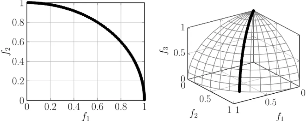
The DTLZ test suite proposed by Deb et al. [64] is perhaps the most welcomed bench-marks in recent research. DTLZ test suite includes seven test problems: DTLZ1 is a biased problem with a linear Pareto front, DTLZ2 is an easy test problem with a spher-ical Pareto front, DTLZ3 is a multi-modal problem and DTLZ4 is a biased problem. DTLZ3 and DTLZ4 have the same Pareto front. DTLZ5 and DTLZ6 are degenerated problem. DTLZ7 has a disconnected Pareto front. DTLZ test suite introduces the idea of scalability, which means the number of objectives are scalable to any number of objec-tives. This is an important feature, which facilitated algorithms investigating into many objective problems.

The WFG suite includes nine test problems, which are also scalable in number of ob-jectives and decision variables as DTLZ test suite. Compared with other test suites, WFG suite is more challenging. The WFG suite introduces attributes such as

(40)

separability/non-disadvantage for WFG test suite is that some of the Pareto front in the suite is too hard to achieve, due to the fact that most of the problems in WFG are non-separable.

2.3

Basic knowledge of Evolutionary Constrained

Multi-objective Optimization

This section introduces the evolutionary approach for constraint multi-objective optimiza-tion, with the discussion of the basic concepts, the existing works and test problems.

2.3.1

Introduction

Algorithms need to optimize more than one objective simultaneously subject to the con-straints in CMOPs. In MOPs, algorithms need to achieve a trade-off between convergence and diversity. As mentioned in Section 2.2 convergence represents whether solutionsare

close to the PF, and diversity represents whether solutions are well spread and covered the whole PF. Unlike MOPs, one more issue, denoted as feasibility, need to be balanced. The feasibility represents whether algorithms can find feasible solutions.

Feasibility maintenance is one of the major tasks for algorithms to handle CMOPs. However, few algorithms have noticed that in some situations, the infeasible solutions are also important to the optimization process. Although solutions located in the infeasible region are not counted as valid output, the infeasible solutions may facilitate the searching process. Figure 2.1 shows two cases. In Case-A, shown in Figure 2.1a, the infeasible region separate the search space into two feasible regions. The infeasible solutions may help algorithms to pass through the infeasible barrier between two feasible regions. In Case-B in Figure 2.1b, there is a infeasible ring between two feasible regions. Without maintaining infeasible solutions in the population, it is hard to converge to the PF.

Generally speaking, it is more challenging to handle CMOPs than MOPs, because algorithms need to achieve the balance among convergence, diversity and feasibility. Con-strained multi-objective evolutionary algorithms (CMOEAs) are particularly designed to

(41)

( a ) C a s e A ( b ) C a s e B

Figure 2.1: Importance of feasibility maintenance

solve CMOPs, with the capability of balancing the search between the feasible and infea-sible areas in the search space [66]. The idea of constraint handling technique is extended from works for the constrained single objective optimization. Unlike constrained single ob-jective optimization, only a few work has been done on solving constrained multi-obob-jective optimization problems. When dealing with CMOPs, the target is to balance convergence, diversity and feasibility simultaneously. Algorithms usually use the constraint violation (CV) to indicate the feasibility of a solution. The CV can be defined in many ways. Usually a solution closer to the feasible region has a smaller CV. One of the commonly used definitions of CV is:

CV(x ) =

p+ q

j= 1

cj(x ) (2.5)

cj is the degree ofj-th constraint:

cj =      |min(Gj(x ), 0)| j ≤p |Hj−p(x )| j > p (2.6)

(42)

No performance indicators are developed for CMOPs in the previous works. In the literature, indicators developed for MOPs are used by ignoring all infeasible solutions.

2.3.2

Methods

Generally speaking, the existing constraint handling techniques for CMOPs can be divided into three groups.

Feasibility-driven algorithms

In this group, feasible solutions are granted a higher priority to survive than infeasible ones. Fonseca and Flemming [67] have developed a framework for solving CMOPs by assigning a higher priority to constraints than to objective functions. The algorithm proposed by Coello Coello and Christiansen simply discards all infeasible solutions [68]. Deb et al. have developed the constrained dominance relation (CDR) for theCMOPs[32]. In CDR, a solutionx1 dominates x2 if 1) x1 and x2 are feasible and x1 Pareto dominate

x2; 2) x1 is feasible while x2 is infeasible; 3)x1 and x2 are infeasible, but CV(x1) < CV(x2). The CDR can simply cooperate with the Pareto dominance relation, which enables all Pareto-based algorithms to handle constraints. Algorithms developed based on CDR such as C-NSGA-II [11] and C-NSGA-III [48] perform well when dealing with constraints. Based on the same principle of CDR, the decomposition-based algorithms also can handle constrained problems using the CV as a prior criterion in the sub-problem update procedure. Several MOEA/D variants [11, 69, 70] have been developed under this idea. Different from CDR [32], Oyama et al. [71] have modified the CDR so that an algorithm prefers solutions violating fewer number of constraints. Takahama et al. [72] and Martnez et al. [73] have proposed an -CDR in which two solutions are considered as equal when the difference of their CVs is smaller than a threshold . Asafuddoula et al. [74] have proposed an adaptive -CDR where the threshold is dynamically adjusted according to the number of feasible solutions.

(43)

Convergence/feasibility balancing algorithms

In this group, algorithms try to achieve a trade-off between convergence and the feasibility. Li et al. [75] have developed a method that keeps solutions in the isolated regions even if they are infeasible. Ning et al. [76] have proposed a constrained non-dominated sorting method, which conducts a second non-dominated sorting with non-domination rank and constraint rank as two objectives. Woldesenbet et al. [77] have extended the idea of penalty function from technique for constrained single objective optimization problems into CMOPs, in which penalties are added to all the original objectives functions.

Feasible maintenance algorithms

In the last group, the algorithms try to avoid infeasible solutions in the reproduction step. Any infeasible solution is driven towards feasible region after generated. Harada et al. [78] have proposed a Pareto descent repair operator that explores possible feasible solutions around infeasible solutions in the constraint space. Jiao et al. Jiao et al. [79] have developed a feasible-guiding strategy in which a infeasible solution is guided moving towards its closest feasible solutions.

2.3.3

Test Problems

Only a few test problems are developed as the test bench for CMOPs. BNH [80], OSY [81], TNK [82], SRN [83], CTP [84] test suite, CF [85] test suite and the C-DTLZ test suite are widely used in the literature.

BNH [80], OSY [81], TNK [82] and SRN [83] are constrained two-objective prob-lems with different types of constraints. BNH test problem has two nonlinear objective functions and two nonlinear inequality constraints. OSY test problem has two nonlinear objective functions, four linear inequality constraints and two nonlinear inequality con-straints. TNK Test problem has two nonlinear objective functions, two linear inequality constraints. SRN test problem has two nonlinear objective functions, one linear inequality

(44)

constraints and a linear inequality constraint.

CTP test problems are have the capability of adjusting the difficulty of the constraint functions. The shape for the PF is not impacted by the constraints in the CTP test problems. The test problem CTP1 gives the difficulty near the PF, because the search area near the PF is infeasible. The constraints for test problems CTP2-CTP8 cause difficulty for convergence in the whole search space.

CF test problems are also commonly used benchmarks. For CF1-CF3 and CF8-CF10, the constraints do not impact the shape of the PF. The constraints only cause difficulty for convergence. The constraints for CF4-CF7 shaped their PFs into many optimal points which lie on some boundaries of the constraints.

2.4

Basic knowledge of Evolutionary Dynamic

Multi-objective Optimization

This section introduces the dynamic multi-objective optimization. The first part gives the introduction. The second part of this section introduces the existing methods solving the DMOPs.

2.4.1

Introduction

Dynamic multi-objective optimization problems (DMOPs) are formally defined by Farina [12] in 2004. Compared with other optimization problems, DMOPs is quite new and haven’t been fully studied. Following the definition in Equation 2.2, types of dynamic are listed as follows:

• Time-dependent constraints. Noted that the changes of constraints can be both changing number of constraints and changing constrained functions. The impact of these two types of changes are the same. The time-dependent decision space also counts in this type, as it is the change of boundaries constraints. It is a very

(45)

interesting research area, however, no existing works have been put efforts on this yet.

• Time-dependent objective functions. The situation of objective functions F varies during the optimization process is the most commonly discussed class of DMOPs. This type of changes are welled studied in the literature, which are commonly found in real world cases. According to Farina et al. [12], the time-dependent objective functions cause four types of impact:

– TYPE I: Moving PF and PS.

– TYPE II: Moving PF, static PS.

– TYPE III: Moving PS, static PF.

– TYPE IIII: Static PF and PS.

• Time-dependent dimension of decision space. n(t) varies in the optimization process. When n(t) varies, the objective functions F must change in the same time. As no works haven been done for the time-dependent time-dependent constraints, no studies have been done on this type of dynamic characteristics.

• Time-dependent dimension of objective space. This is caused by adding or removing objective functions during the optimization process. Although changing number of objectives happens widely in real-life, this type of dynamic is nearly untouched.

The framework of dynamic handling technique for DMOPs is shown in Figure 2.2.The main steps of the dynamic handling technique are reconstruction, reproduction and se-lection.

When a change is detected, algorithms react to the changes by reconstructing the population. There are plenty of reconstructing strategies being proposed in the literature. The simplest idea is reconstructed the population with random solutions [9, 86, 87]. The works based on this method usually focus on two problems: 1) how many solution need

(46)

Figure 2.2: Framework of dynamic handling technique

[88–96]. According to the historical PF or PS, the algorithms use mathematical model to predict the new PF or PS. Then algorithms reconstructed the population around the predicted PF or PS. This type of methods performs well on handling the moving PS or PF. Some others based on the recorded previous optimal [97, 98], the algorithms set a “state” every time the problem is changed and recorded the best solution(s) for every state. Once the algorithms find the problem turns back to a recorded state, the recoded best solution(s) is/are used to reconstruct the population. This type of method performs well on the DMOPs with a periodical change, which means the PS/PF is expected to return to the same position in the future. Unlike the reproduction only change the population once, the reproduction and selection can continuously impact the population for a long term after the change. One typical example based on this method is the D-NSGA-II [9], which does not reconstruct the population after the changes, but replaces part of the population with random solutions in the selection.

2. 4. 2

M

e t h o d s

In this section, we introduce the current dynamic handling method for DMOPs. Noted that only time-dependent objective functions have been studied. All these works are about this type of dynamics. The existing dynamic handling techniques can be classified into three categories:

• Diversity enhancement: The basic idea of this category is injecting new solutions

(47)

new solutions, the solutions in the population are likely to jump out of the current optimum position and move towards the new PF. Diversity enhancement can be di-vided into two subcategories according to the timing of injecting new solutions. One is responding to the dynamics after a change is detected, which is known asdiversity introduction. Some works [9, 99, 100] propose hyper-mutation methods which help the solutions in the population jump out of their current positions, thus to handle the dynamics. In some other works [9,86,87], solutions generated either randomly or specifically by some heuristic methods are injected into the current population. All these new solutions participate in the survival competition together with the exist-ing ones. The other subcategory is maintainexist-ing the population diversity durexist-ing the whole process, which is called diversity maintenance. Unlike diversity introduction,

diversity maintenance does not respond to dynamics explicitly. It mainly relies on the diversity maintenance strategy to track the moving PF. Multi-population strategy [101] is also designed to enhance the population diversity.

• Memory mechanism: The basic idea of memory mechanism is accelerating the con-vergence progress with the help of historical data. This method only works when the PS moves periodically, which means the PS is expected to return to the same position in the future. Wang et al. [97] have proposed a hybrid memory scheme which relocates the new population either by the previous non-dominated solution or by a local search on the archive. Peng et al. have [98] exploited the historical knowledge and uses it to build an evolutionary environment model. This model serves to guide the adaptation to the changing environment.

• Prediction strategy: The idea for this type is to predict the location of the new PS and rebuild the population in that location. It can be regarded as an upgraded version of memory mechanism. Instead of directly using the historical solutions, the algorithm uses historical information to predict the future location of the PS. For example, works from Hatzakis et al. [88, 89] employ an autoregressive model to

(48)

track the new PS population within the neighbourhood. By utilizing the regularity property [90], Zhou et al. [91, 92] and Peng et al. [93] have built a model for the movements of the PS manifolds’ centres under different dynamic environments. Wu et al. [94] and Koo et al. [95] have proposed to predict the optimal moving direction of the population. More recently, Murugananth et al. [96] have proposed a hybrid scheme, which uses either the Kalman Filter or random re-initialization based on their performance.

2.4.3

Performance Indicators

Most of the indicators for dynamic multi-objective optimization are extended from the indicators for multi-objective optimization. The indicators can be classified into three types. To be brief, we denoted the indicators for MOPs as static indicators.

• The performance at the end of optimization also can be used to indicate the per-formance for the algorithms handling DMOPs. Ignoring all the situations during the optimization process, the performance indicator only measure the final outcome. Any indicators developed for multi-objective optimization can be used. For example:

Final IGD(FIGD): P_tmax∗ is a set of points uniformly sampled along the P Ftmax,

Stmax is the set of solutions obtained by an EMO algorithm for approximating the

P Ftmax, and tmax is the final time step in a run,

FIGD=IGD(Ptmax∗ ,Stmax). (2.7)

• Mean value before changes calculates the mean value of the indicators developed for MOPs before every change. Indicators in this type mainly focus on how well the algorithms recover from the changes. For example:

Mean IGD(MIGD):P_t∗ is a set of points uniformly sampled along theP Ft,St is the

(49)

is a set of time steps, which are one step before every changes in a run, MIGD= 1 |T| X t∈T IGD(Pt∗,St). (2.8)

• We also can calculate the integration of the value of an indicator during the whole optimization process, instead of using the value at time steps before changes. This type of performance indicators focuses on how quick the algorithms recover from the changes. For example:

Integrated Inverted Generational Distances(IIGD): P_t∗ is a set of points uniformly sampled along the P Ft, St is the set of solutions obtained by an EMO algorithm

for approximating the P Ft.tbegin ≤ t ≤tend, tbegin and tend is the starting time and

ending time for the optimization process.

IIGD= 1

|T|

Z tend

tbegin

(50)

CHAPTER 3

DYNAMIC TWO-ARCHIVE EVOLUTIONARY

ALGORITHM

Most existing research focus on the dynamic multi-objective optimization problems (DMOPs) with time-dependent objective functions, whereas DMOPs with a changing number of ob-jectives have seldom been considered yet. DMOPs with a changing number of obob-jectives can be found in many real-life scenarios, such as software project scheduling and operations management. Time-dependent objective functions usually lead to the change of shape or position of the Pareto-optimal front/set. However, the increase/decrease in the number of objectives always results in the expansion or contraction of the dimension of the Pareto-optimal front/set manifold. Unfortunately, most existing research can hardly handle this type of dynamics. This chapter begins with the definition of dynamic multi-objective op-timization problems with a changing number of objectives. Then a dynamic two-archive evolutionary algorithm (DTAEA) is implemented to tackle this problem. DTAEA main-tains two populations simultaneously. For each population, there are different updating and reconstructing strategies, with a mating strategy proposed. Last,sevenother research questions will be discussed and analysed.

This chapter is organised in the following way. Section 3.1 clarifies the motivation. Section 3.2 probes DTAEA and its implementation. Experimental results of DTAEA are presented in Section 3.3. Further research questions and analysis of the DTAEA are carried out in Section 3.4. Finally, Section 3.6 summarises this chapter.

(51)

3.1

Motivation

Multi-objective optimization, which can often be found in real-life scenarios (e.g. engi-neering [102], economics [103], and logistics [104]), tries to achieve the trade-off among two objectives or more simultaneously. Due to the conflicting nature of the objectives, it is impossible to obtain a solution optimizing all objectives. Instead of finding one solution, the best trade-off solutions among those objectives, known as Pareto optimal solutions, have aroused the interest of the decision makers. In real-life optimization scenarios, a dynamic incident happens uncertainly. For example, in a production line, new jobs arrive over time and machines in the production line breakdown from time to time [105]. An-other example can be found in a design process. The quality of the raw material changes in the production process [106]. Generally speaking, dynamic optimization problems are usually more challenging than those stationary ones, because the algorithm needs not only to achieve trade-off solutions, but also to deal with the changes. An effective dy-namic multi-objective optimization algorithm should be able to track the time-dependent Pareto-optimal front. Evolutionary Algorithm (EA) is known as a powerful and popu-lar tool to handle dynamic multi-objective optimization [8, 9, 12, 99, 100]. The existing dynamic handling techniques can be classified into three categories:

• Diversity enhancement: Diversity includes two aspects: 1) cover the whole Pareto-optimal front (PF), 2) well spread the population on the PF. The basic idea of this category is injecting new solutions into a converged population to increase the diver-sity. With the guidance of these new solutions, the solutions in the population are likely to move twards the new Pareto-optimal front from the current optimum posi-tion. Diversity enhancement can be divided into two subcategories according to the timing of injecting new solutions. One is responding to the dynamics after a change is detected, which is known as diversity introduction. It is usually accompanied with a change detectio