An Adaptation Reference-point-based Multiobjective Evolutionary
Algorithm
Juan Zoua,b,c, Liuwei Fuc,∗, Shengxiang Yange, Jinhua Zhengc,d, Gan Ruanc, Tingrui Peia, Lei Wangc
aKey Laboratory of Hunan Province for Internet of Things and Information Security, Xiangtan University, Hunan Province, China bLED Lighting Research & Technology Center of Guizhou TongRen, GuiZhou, China
cKey Laboratory of Intelligent Computing and Information Processing, Ministry of Education, Xiangtan University, Xiangtan, Hunan
Province, China
dHunan Provincial Key Laboratory of Intelligent Information Processing and Application, Hengyang, 421002, China eSchool of Computer Science and Informatics, De Montfort University, Leicester LE1 9BH,U.K.
Abstract
It is well known that maintaining a good balance between convergence and diversity is crucial to the perfor-mance of multiobjective optimization algorithms (MOEAs). However, the Pareto front (PF) of multiobjective optimization problems (MOPs) affects the performance of MOEAs, especially reference point-based ones. This paper proposes a reference-point-based adaptive method to study the PF of MOPs according to the can-didate solutions of the population. In addition, the proportion and angle function presented selects elites during environmental selection. Compared with five state-of-the-art MOEAs, the proposed algorithm shows highly competitive effectiveness on MOPs with six complex characteristics.
Keywords: Multiobjective optimization; Many-objective optimization; evolutionary algorithms; genetic
algorithms;
1. INTRODUCTION
1
Recently, multiobjective evolutionary algorithms (MOEAs), have been proposed to solve multiobjective optimization problems (MOPs) [39]. Generally, MOPs, which involve more one conflicting objective to be optimized, can be formulated as follows:
min
x∈DF(x) = (f1(x), f2(x), . . . , fM(x)) T,
(1) whereD⊆Rnis the decision space;x= (x
1, x2, . . . , xn)∈Dis the decision variable;M ≥2is the number
2
of the objectives, and F consists of M objectives. The rapid development of MOEAs directly reflects the
3
need to handle MOPs in real-world scenarios, such as in optimizing visualization [23, 8, 25], traffic control
4
[65][31], control system design [51][19], and industrial planning [1, 20, 22, 24]. MOEAs can find a set of
5
∗Corresponding author: Liuwei Fu
optimal solutions (rather than a single one) in an evolutionary manner and have performed excellently on
6
various MOPs.
7
In the development of MOEAs, Pareto-based approaches, such as dominance relation and density
estima-8
tion, are first used to optimize MOPs. dominance relation selects a solution by the objectives’ values and
9
provides selection pressure toward the Pareto front (PF). Density estimation is used to maintain diversity
10
when some solutions are non-dominated according to the dominance relation.Deb et al.[34] proposed the
11
non-dominated sorting generic algorithm II (NSGA-II) for conflicting problems. The NSGA-II has two main
12
phases: first, a nondominated sorting approach is used to create Pareto rank; then a crowding distance is
13
applied to implement density estimation. Zitzler et al.[16] modified the density estimation and presented an
14
enhanced archive truncation method. However, it is a problem that Pareto dominance-based methods lead to
15
the severe loss of selection pressure on the PF as the number of objectives increases. The primary reason
be-16
hind the failure of Pareto-based MOEAs is the large increase of non-dominated solutions [53]. Another major
17
reason is that the diversity of a population is hard to maintain with the limited population size in MOPs. Some
18
studies have pointed out the drawback of Pareto-based algorithms [39][7][63]. To overcome the drawback of
19
Pareto-dominance-based MOEAs, relaxed-dominance-based approaches have been proposed, such as epsilon
20
dominance [45][44], favor relation [69][49], fuzzy Pareto dominance [43][3], particle swarm[61][26][50],
21
and SDE [47].
22
Indicator-based approaches adopt a performance indicator to optimize a desired ordering among the
23
population set during the evolution. These approaches seem to be a direct way to solve MOPs. Among the
24
current indicators available, the indicator-based EA (IBEA) [14] uses a single indicator to guide the search
25
process. The hypervolume (HV) [13] is probably the most popular performance indicator in multiobjectve
26
search due to its potential to balance convergence and diversity. A number of well-established indicator-based
27
MOEAs that employ the theoretical properties of HV are available, such as the S metric selection evolutionary
28
algorithm (SMS-EMOA) [48] and multiobjective covariance matrix adaptation evolution strategy
(MO-CMA-29
ES) [10]. Nevertheless, there are two downsides to indicator-based MOEAs in handling MOPs[62]. One is
30
that the computational cost of HV grows exponentially with an increase in the number of objectives [36].
31
The other is too much selection pressure, which produces inferior performance in terms of distribution on
32
the PF [46] [11]. In such conditions, the HV prefers to choose the knee and border of the PF rather than the
33
points having more diversity [4][68]. To relieve the computational cost of HV, researchers use the indicator
34
values of estimated HV to improve efficiency. For example, the hypervolume estimation (HypE) algorithm is
35
widely applied in high-dimensional optimization problems by using a Monte Carlo simulation [42]. Recently,
36
methods using several other performance indicators as a substitute have achieved similar results to those
37
using the HV in the evolutionary process. For example, R2 and additive approximation [57][5].
38
Decomposition-based approaches divide complex MOPs into a set of single-objective sub-problems through
39
aggregation functions, and then solve them simultaneously in a collaborative manner. The evolution
tion of a sub-problem is guided by specifying a set of well-distributed reference points that maintain the
41
population’ diversity [59][6][66]. Decomposition-based approaches can be directly applied to the selection
42
mechanism of MOEAs by a single scalar value rather than pareto dominance. Generally, weight vectors and
43
the aggregation function are critical to decomposition-based approaches [40][67][38]. Weight vectors affect
44
the distribution of the solutions in the objective space, and guide the evolutionary direction. The
aggrega-45
tion function provides the mechanism to update individuals in the selection strategy. Recently, two types
46
of decomposition-based approaches were classified [64]. The first type divides MOPs into a set of
single-47
objective problems (SOPs). For example, Multiple Single Objective Pareto Sampling(MSOPS) and MOEA
48
based on decomposition (MOEA/D) [52],NSGA-III [33]. The second type of decomposition-based approach
49
divides MOPs into a set of sub-MOPs. For example, a multiobjective evolutionary algorithm using dynamic
50
weight design method (MOEA/D-M2M) [17]. Although decomposition approaches have become popular due
51
to their efficiency [47], they encounter difficulty in handing an irregular PF [7].
52
Although many decomposition approaches based on adaptation have been proposed to solve MOPs with
53
irregular PFs, it is hard to maintain a balance between convergence and diversity. Motivated by the ideas,
54
we propose a new adaptation reference-point-based optimization algorithm, (ARMA), for solving MOPs.
55
Compared with existing reference-point-based methods, the main contributions of this paper are as follows:
56
• A hyperplane learning strategy is proposed to adjust the relative position of reference points to deal
57
with MOPs that have a concave or convex PF. The proposed strategy uses a parameterϕto control the
58
hyperplane shape of the reference points according to the objective value of a whole population so that
59
the distribution of solutions can be improved.
60
• The new clustering method is designed to balance the niche-preservation operation in multiobjective
61
optimization according to the reference points. We divide a population into a number of niches by value
62
of the proportion and angle, and then select a better solution in the niche. In this method, convergence
63
and diversity are primarily measured by proportion and angles.
64
The remainder of this paper is organized as follows. Section II reviews related work. The details of the
65
proposed ARMA are described in Section III. Section IV present results and an investigation of multiobjective
66
problems. Further discussion of parameterϕbehavior is given in Section V. Finally, conclusions are drawn in
67
Section VI.
68
2. RELATED WORK
69
Reference point-based MOEAs have been proposed in which the quality of the population is measured by a
70
set of reference points. Two phases (constructing a reference set and measuring the quality of the population)
71
are the main methods used in reference-point-based approaches. In NSGA-III [33][29], the reference points,
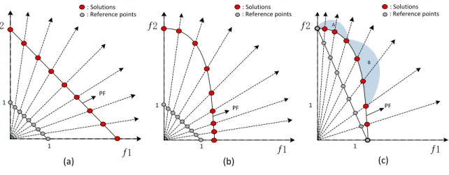
(a) Х Х 1 1 (b) Х Х 1 1 Х Х 1 1 (c) : Solutions : Reference points PF A B PF PF : Solutions : Reference points : Solutions : Reference points
Figure 1: Pareto-optimal solutions (red solid dots) specified by different reference points (grey solid dots). (a) Pareto-optimal solutions specified by nine uniformly distributed reference points on a PF with the same range.(b) Pareto-optimal solutions specified by nine uniformly distributed reference points with differently scaled.(c) Pareto-optimal solutions specified by nine adapted reference points in the RVEA algorithm.
using Das and Dennis’s systematic approach [27], are predefined to ensure the population’s diversity.
NSGA-73
III’s selection strategy uses the Pareto dominance relation and decomposition operator to balance convergence
74
and diversity in the evolutionary process. In RVEA [54], a scalarization approach using angles and distances
75
is adopted to measure solutions. In a strength pareto MOEA based on reference direction (SPEA/R) [58],
76
a reference vector-based local fitness assignment scheme preserves the most promising individual in the
77
subregion. Tian et al.[60] adapted the position of the reference point to preserve extreme solutions for better
78
diversity. In indicator-based MOEA (AR-MOEA), an excellent individual from the archive is used to replace
79
the poorly distributed reference point and serves as the reference point to guide the evolutionary search.
80
Reference-point-based MOEAs maintain the distribution of the population through a clustering strategy
81
using reference points as shown in Fig. 1(a). In general, the diversity of predefined reference points is crucial
82
to the PF. Das and Dennis’s systematic approach, which places points on af1+f2+· · ·+fM = 1hyperplane,
83
is adopted in most MOEAs to generate the predefined reference points[9][56]. However, in Fig . 1(b), it is
84
difficult to generate uniform reference points on differently scaled PF of MOPs, as is the case in the WFG test
85
problems[55] and the scaled DTLZ problems [35] which have various features. Different scale optimization
86
problems cause great difficulties for reference-point-based selection strategies.
87
There are two methods to address this issue. One is that objective normalization dynamically is
intro-88
duced as the search proceeds, as in NSGA-III, SPEA/R andθ-DEA. The other is to adapt the reference points
89
according to the ranges of the objective values. In RVEA, reference point adaptation is used to deal with the
90
badly-scaled PF in Fig. 1(c). These two methods have obtained better performance on the scale problem.
However, these methods do not achieve a relatively uniform distribution of solutions when coping with
92
a non-planar PF, especially concave and convex PFs. From Fig. 1(c), it can be seen that the individual
93
distributions of areas A and B perform differently. Compared with the A area, solutions in the B area are too
94
sparse. Maintaining the diversity in the peak of the PF is becoming a new challenge for reference point-based
95
MOEAs.
96
3. PROPOSED ALGORITHM
97
The basic framework of the proposed ARMA is described in Algorithm 1. At the beginning of ARMA, the
98
population is initialized randomly and the reference points are constructed using Das and Denis’s
system-99
atic approach and T wo-layer methods. In each iteration, the parent population reproduces its offspring by
100
crossover operation and mutation operation. Then, the parent and offspring are integrated into the double
101
population. Next, in order to handle problems with disparately scaled objectives, the adjustment strategy
102
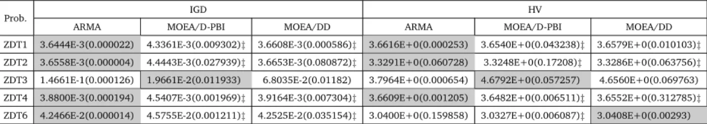
dynamically adjusts the distribution of reference points according to the obtained solution on the
approx-103
imated PF. Then the solution in the double population applies proportion [41] and angle to link up with
104
one reference point. The double population is partitioned intoN different subpopulations, whereN is the
105
number of the population. The proportion and angle are described in subsection B. After the clustering
op-106
eration, the candidate solution with the smallestF itnessvalues is chosen in the environmental selection. In
107
the following sections, the important procedures of the ARMA are described in detail.
108
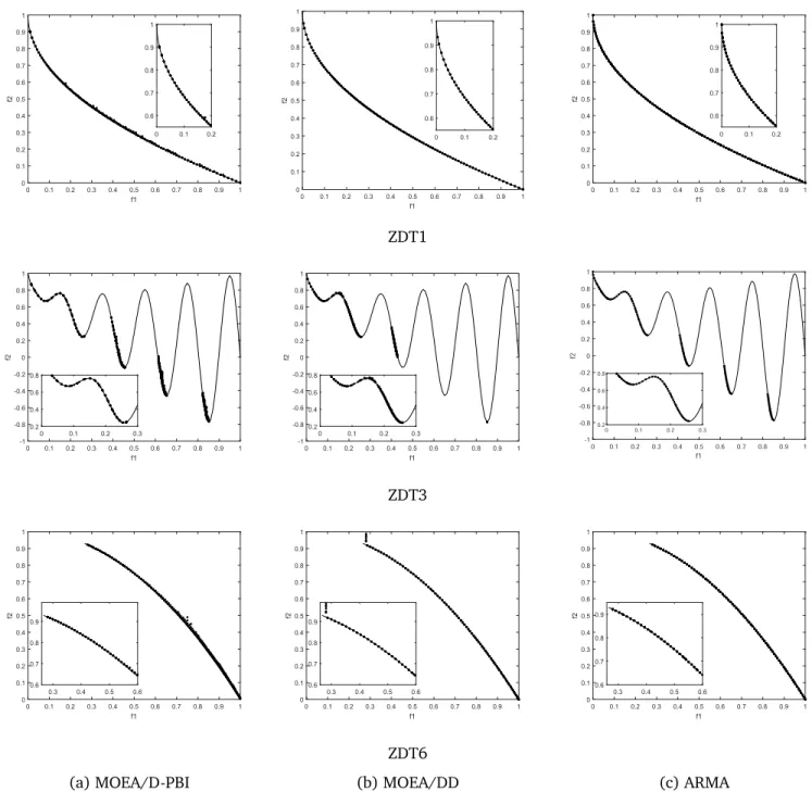
3.1. Adaptive Methods
109
We are proposing new adaptation methods which comprise two steps to maintain the diversity of reference
110
points. First, the reference points are adjusted for the scale problems and form the approximate shape of the
111
PF by using the parameter ϕ. Further performance of parameterϕ is described in Section V. Second, the
112
relative position of the reference points must be reevaluated by its neighbor.
113
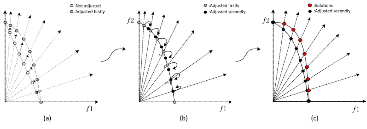
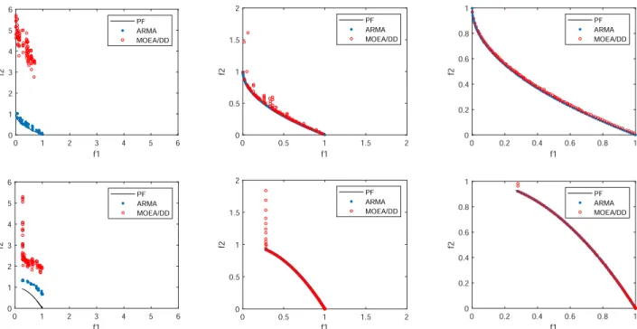
In the early period, the maximum values of each objective function is obtained to deal with badly-scaled PF in RVEA, but the worst individual in the population severely affects this implementation and fluctuates strongly in the maximum values. Thus, we use small steps to readjust the reference point. The detailed introduction of small stepSand reference point adjustment are in equation (2).
S=argmin(Zjmax−Zjmax−1),1< j≤M, (2)
where Zjmax denotes the maximum values ofjthobjective function;M is the number of objectives; and S is the increment in the objective. Therefore, the maximum value of each objective function is readjusted as follows:
Algorithm 1Framework of ARMA
Input: N(population size)
Output: The approximated Pareto-optimal front
1: Λ :=Generate-Reference-Points().
2: P0←Initialize-Population().
3: t←0.
4: whilethe termination criterion is not metdo
5: Qt:=Make-Offspring-Population(Pt).
6: Rt:=Pt∪Qt.
7: Λ :=Adaptation-Reference-Point(Pt).
8: Compute the proportion and angle of the population and reference points, respectively.
9: foreach solutioniinRtdo
10: AssociateRt,iwith reference point according to the proportion and angle.
11: end for
12: foreach reference pointjϵΛdo
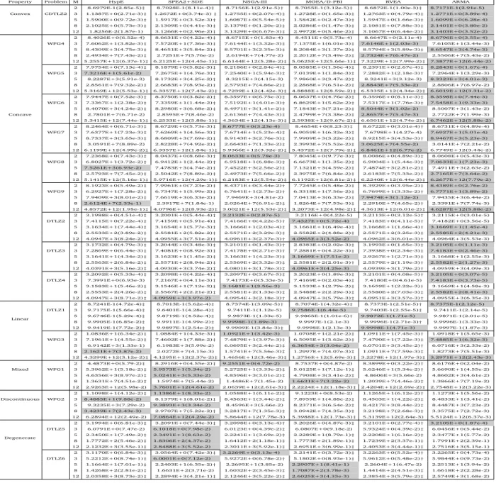
13: CalculateF itnessvalues of solution injth Niching.
14: Select the solution with smallestF itnessintoPt.
15: end for
16: end while
where modifiedZmax′
j is the maximum value ofjthobjective function. After that, the relative position of the reference point is adjusted by the vectorZt = (Zmax
′
1 , Z
max′
2 , . . . , Z
max′
m )for the first time in the following manner:
Rt,i =R0,i◦Zt,1< i≤N, (4)
whereRt,i denotes theith adapted reference point in thetgeneration ;R0,idenotes theith reference point generated in the initialization stage;Nis the number of the reference points, and the′◦′operator denotes the Hadamard product, which wisely multiplies two matrices of the same size. In order to make the reference point satisfy the situation that the surface of the PF is curved, as shown in Fig. 2(a), the reference point movesϕlength of the distance between the reference point and the nearest individual in its niche along the direction of the origin and the current reference point.
Rt,i=Rt,i(||
Rt,i||+ϕD
||Rt,i|| ), (5)
where Dis the distance between the reference point Rt,i and the individual inRt,i niche. The hyperplane
114
that the modified reference points make up is pretty similar to the shape of the PF. However, the distribution
115
of the reference points on the hyperplane is not as evenly even as before the modification process in Eq (5).
116
The second modification process is therefore required to make the reference points distribute evenly on the
Х (c) Х Х Х (a) Х Х r (b) r+1 r-1 :Adjusted secondly :Adjusted firstly
:Not adjusted :Adjusted firstly :Solutions
:Adjusted secondly
Figure 2: Adaptation reference points according to the solutions obtained. (a) nine reference points move to PF. (b) adjusting the reference points according to theirmneighbor. (c) Pareto-optimal solutions specified by nine adapted reference points.
hyperplane. The detailed adjustment process of the reference points is as follows. First, for each reference
118
point, the m neighbor is selected with maximum distance from the 2m neighbor, where the 2m nearest
119
neighbor reference points along positive and negative directions of the coordinate axis are found. Then, the
120
average values of all points’ Euclidean distances from the points to their m neighbors in mdirections are
121
calculated. If there are not any reference points in the positive direction for some reference points, take the
122
boundary points for example, a value of average is assigned. Lastly, two reference pointsAandB with the
123
largest distance in themth objective are selected. In order to make their distance reach the average, A is
124
adjusted to moveB, andAandBare marked, whereBmust meet the following conditions:
125
• condition 1:Bhas a value of 0 in themth objective (boundary point).
126
• condition 2:Bis marked.
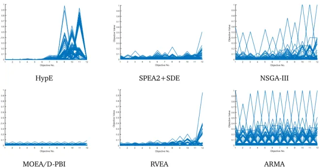
127
• condition 3: if conditions 1 and 2 are not satisfied,Bis randomly selected fromAandB.
128
This way, each reference point has the same approximate distance from its neighbors, thus having uniform
129
distribution. The detailed procedure is introduced in Algorithm 2.
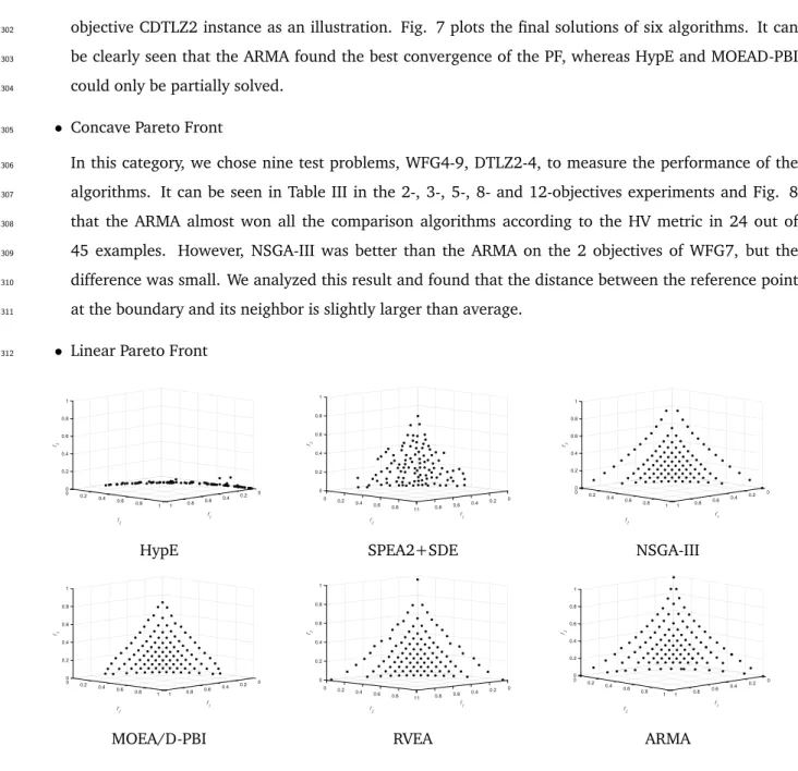
130
It is worth emphasizing that the proposed adaptation method is different from other
reference-point-131
based evolutionary algorithms, such as indicator-based MOEA (AR-MOEA). Compared with AR-MOEA, the
132
proposed adaptation method adjusts reference points to form an approximated PF in this paper. In addition,
133
the relative positions of the reference points are reevaluated by their neighbors. However, the goal of
AR-134
MOEA is to preserve the extreme solutions for better diversity in the adjusting approach.
Algorithm 2Reference Adaptive
Input: t(generation index),Pt(populationPt)Λ(unit reference point);
Output: adaptive reference pointΛ’ for current generation;
1: Calculate the minimumSand maximal valuesZtmaxby Eq.(1); 2: fori = 2 to Ndo 3: Zmax i ′=Z1max+ (i−1)·S 4: end for 5: fori = 2 to Ndo 6: Ri′=Ri◦Zmax i ′ 7: end for 8: fori = 1 to Ndo 9: R′′i =R′i•( ||R′i||+ϕD ||R′i|| ) 10: end for
11: Find the averageavgfrom all the points to theirmneighbors.
12: Find the individualpwhich has the bigger Euclidean distance from its neighbor.
13: Queues←p.
14: whilesis not emptydo
15: p:=sdequeue.
16: Adjustp’s Euclidean distance from its neighbor according to theavg.
17: s←p’s neighbor.
3.2. Selection Strategy
136
There are many ways to divide the entire population intoN subpopulations according to the reference
137
points. In NSGA-III, the perpendicular distance between each solution and reference point is presented.
138
In RVEA, the angle between the solution and reference point is used to complete the clustering operation.
139
Compared with the aforementioned approaches, the ARMA partitions the population intoN subpopulations
140
using the approximation of proportion and angles, and the selection strategy is implemented separately in
141
each subpopulation. The proportion and angles method can effectively avoid the impact of non-normalization
142
and form a mapping relationship between reference points and the individual to complete the partition in
143
the objective space. Thus, this method does not focus on a solution that is closed to the reference point but
144
emphasizes the center of the population. In the proposed ARMA, the environment environmental selection
145
operation comprises two steps: calculating the proportion and angle, and selecting an elite individual inside
146
the subpopulations.
147
3.2.1. Calculating the proportion and angle
148
The center of population, or reference sets, denoted asCP orCR, could be estimated by the objective
149
value of each individual or reference point. The proportion ofi-th reference point, denoted asP Ri, can be
150 calculated as
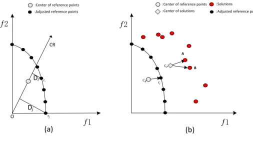
(a)
Х
Х
Di Dj:Center of reference points :Adjusted reference points
ri r O CR A B C C r!
(b)
Х
Х
:Solutions:Adjusted reference points :Center of reference points
:Center of solutions
Figure 3: Example showing the calculation of the proportion and angle.
151
P Ri=
Di
max(D1, D2, . . . , D2N)
, (6)
whereiis thei-th reference point, andDi is the perpendicular distance from the reference pointi-th to the
152
center vectorCRfrom the origin to center as shown in Fig. 3(a). The proportion of an individualPi, denoted
asP S, can be calculated using the same methods.
154
The angle between vector−−−−−→ri−CRand vector−−−−−→f−CP can distinguish the relationship whether they have the same direction or not.fis an individual in the population. The−−−−−→ri−CRand the
−−−−−→
f −CPcan be considered
as the same direction vector if they have the smallest angle. Given two vectors, a large cosine value means a smaller angle. The cosine value can be calculated as
cosθi,j= −−−−−→ fj−CP · −−−−−→ ri−CR ||fj−CP|| · ||ri−CR|| , (7)
whereθi,jis the angle between the−−−−−→ri−CRand the−−−−−→f−CP.
155
3.2.2. Selecting an elite individual inside the niche
156
Population Pt is divided into N niches according to the proportion value and angle. Individual f is
157
allocated to a reference pointrif the angle and difference of proportion|P Sf −P Rr|between individualf
158
and reference pointris minimal. P Sf andP Rr is the proportion off andr, respectively. In other words,
159
individual f and reference point r, which have the smallest angle and proportion difference, are linked
160
together.
161
After partitioning the population, it becomes important to select individuals from the subpopulation. Most current algorithms based on reference vectors use the distance or angle between the individual and the reference vector to select candidate individuals. In this paper, we propose an approach as
F itnessf,r=Distancef,r+Anglef,r+|P Sf−P Rr|, (8)
whereDistance(Angle) is the Euclidean distance (angle) between the individual and reference point in the
162
niche, respectively. P Sf andP Rrare the proportion of individualf and reference pointr.
163
TheF itness function is designed to meet the convergence and diversity criteria. In the early stage of
164
theF itnessfunction, providing strong convergence pressure makes the population quickly converge to the
165
PF during the evolutionary process. Distancef,r plays a decisive role in the convergence so that the whole
166
population can converge to the PF quickly. At a later stage, the mechanism of Anglef,r +|P Sf −P Rr|
167
becomes more crucial than the convergence and provides a uniformly distributed solution set for decision
168
makers. This means that the diversity criterion strongly affects the value ofF itnessand plays a decisive role.
169
In addition, although the solution sets are not evenly distributed in the early stage, the population is divided
170
intoN niches in the early evolutionary process, which roughly guaranteed the distribution. The balance of
171
convergence and diversity can be maintained by selecting the elite individuals based on the smallerF itness
172
value in each niche.
173
3.3. Computational complexity of the ARMA
174
In order to analyze the computational complexity of the ARMA, we only consider the main steps and
175
processes in one generation in Algorithm 1. The computational complexity of ARMA is composed of two
Algorithm 3Selection Strategy
Input: Pt(population),Λ(unit reference point);
Output: PopulationPt+1for next generation;
1: /*The perpendicular specific value of the Population and reference point*/
2: Calculate the proportion valueP RandP S; refer to (5).
3: /*Population Partition*/
4: fori=1 to|Pt|do
5: forj=1 to|Λ|do
6: Calculate the anglecosθi,jbetween−−−−−−→Pt,i−Cpand−−−−−→Rj−Crby Eq.(6)
7: end for
8: end for
9: fori = 1 to|Pt|do
10: Individual link to the reference point according the proportion and angle;
11: end for
12: /*Elitism Selection*/
13: forj = 1 to Ndo
14: Selecting the elite solution with smallestF itnessfrom niche by Eq.(7).
15: end for
parts: reference-point adaptation and environmental selection.
177
In Algorithm 2, the computational complexity of the reference points’ adaptation isO(M N2)when all the
178
reference points need to be adjusted;N is the number of solutions, andM is the number of the problem’s
179
objectives. In addition, environmental selection consists of partitioning the population and the elite selection.
180
In population partition, the proportion and angle calculations takeO(2M N)andO(M N2)in the worst case,
181
respectively. Finally, the calculation ofF itnessand elite selection just spendsO(2N)in a niche in the worst
182
scenario.
183
Therefore, the worst case average computational complexity of ARMA within one generation isO(M N2),
184
which is as efficient as RVEA and NSGA-III.
185
4. Comparative Studies
186
4.1. Performance Metrics
187
In order to test the performance of the algorithm in the experiment, we used the well-known indicators
188
IGD [21] and HV [13]. The details of IGD and HV are introduced next.
4.1.1. Inverted Generational Distance
190
Inverted generational distance (IGD) can test the population obtained by the MOEA convergence infor-mation and distribution inforinfor-mation simultaneously. LetAbe a set of solutions uniformly sampled from the true PF, andP∗be the approximated solutions in the objective space. The IGD calculated as follows:
IGD(A, P∗) = 1 |P∗| v u u t∑|p∗| j=1 e d2 i, (9)
wheredi(dei) is the Euclidean distance between thei-th member in setAand its nearest member in setP∗.
191
4.1.2. Hypervolume
192
The HV metric is used to measure the volume of the objective space. In general, HV can measure both the convergence and diversity of a solution set in the last generation. LetP∗ be a set of approximated solutions in the objective space, andr=(r1, r2, . . . , rm)T be a reference point which is dominated by all individuals in setP∗. The HV is calculated as follows:
HV(P∗, r) =volume ( ∪ f∈P∗ f[f1, r1]×. . .[fm, rm] ) , (10)
In addition, we calculated HV exactly using the recently proposed WFG algorithm [42] for problems with no
193
more than 8 objectives. The Monte Carlo simulation proposed in [32] was adopted to approximate the HV
194
for problems having 12 objectives, and 10,000,000 sampling points were used to ensure accuracy.
195
4.2. Experimental Settings
196
4.2.1. Reproduction Parameters
197
For the comparison in the experiment, all simulated binary crossover and polynomial variations in the
198
algorithms’ settings were the same. The crossover probability and its distribution index were pc=1.0 and
199
ηc = 20. Similarly, the polynomial mutation probability and distribution were set topm= 1/n andηm=20,
200
respectively.
201
4.2.2. Population Size
202
The population size in 2-, 3-, 5-, 8- and 12-objectives was set to 100, 105, 126, 120, 110, respectively.
203
4.2.3. Termination Condition
204
The termination condition is set according to the maximum generation. The maximum number of
gen-205
erations was set to 500 for ZDT suites problem, and for the DTLZ and WFG suites problems, the maximum
206
generation was 1000. In addition, each algorithm ran independently 30 times for each problem.
4.3. Performance on Multiobjective Optimization problems
208
4.3.1. Test Problems and Other Algorithms in Comparison
209
In order to study the performance of the ARMA algorithm on multiobjective problems, the test problems
210
ZDT1, ZDT3 and ZDT6 were selected from the ZDT suites [15]. The ZDT multiobjective problems contain
211
two objectives and all scaled decision variables. They were used to test the ability of MOEAs on the two
212
objectives. ZDT1 has a convex PF with different partial constraints. ZDT3 is a non-continuous, convex PF
213
test problem and poses a great challenge to the MOEAs.
214
The ARMA algorithm is a point-based decomposition algorithm instead of being
reference-215
vector-based, so we chose MOEA/DD [37] and MOEA/D as contrasting algorithms for the multiobjective
216
problems. MOEA/D is representative of the decomposition algorithm, and it has advantages in
multiobjec-217
tive algorithms. MOEA/DD exploits the merits of both dominance- and decomposition-based approaches to
218
balance the convergence and diversity of the evolutionary process.
219
Table 1: MEAN AND STANDARD DEVIATION IGD AND HV VALUES ON ZDT PROBLEMS
Prob. IGD HV
ARMA MOEA/D-PBI MOEA/DD ARMA MOEA/D-PBI MOEA/DD
ZDT1 3.6444E-3(0.000022) 4.3361E-3(0.009302)‡ 3.6608E-3(0.000586)‡ 3.6616E+0(0.000253) 3.6540E+0(0.043238)‡ 3.6579E+0(0.010103)‡
ZDT2 3.6558E-3(0.000004) 4.4443E-3(0.027939)‡ 3.6653E-3(0.080872)‡ 3.3291E+0(0.060728) 3.3248E+0(0.17208)‡ 3.3286E+0(0.063756)‡
ZDT3 1.4661E-1(0.000126) 1.9661E-2(0.011933) 6.8035E-2(0.01182) 3.7964E+0(0.000654) 4.6792E+0(0.057257) 4.6560E+0(0.069763) ZDT4 3.8800E-3(0.000194) 4.5407E-3(0.001969)‡ 3.9164E-3(0.007304)‡ 3.6609E+0(0.001205) 3.6482E+0(0.006511)‡ 3.6552E+0(0.312785)‡
ZDT6 4.2466E-2(0.000014) 4.5755E-2(0.001211)‡ 4.2525E-2(0.035154)‡ 3.0400E+0(0.159858) 3.0327E+0(0.006087)‡ 3.0408E+0(0.00293)
‡and†indicate ARMA performs significantly better than and equivalently to the corresponding algorithm, respectively.
4.3.2. Results on Multiobjective Optimization Problems
220
The mean and standard deviation values of IGD and HV of the current population were used to evaluate
221
the ARMA, MOEA/DD, and MOEA/D-PBI, where the best value for each problem is marked in grey
back-222
ground. In addition, in order to accurately analyze the statistical results, the Wilcoxon rank-sum test was
223
carried out to indicate the significance between different results at the 0.05 significance level in multiple
224
comparisons [18].
225
In the ZDT test suite, ZDT3 is the only disconnected problem. Table I shows that the ARMA performs, in
226
terms of the number of the function evaluations, significantly better than MOEA/DD and MOEA/D-PBI on
227
most of the test problems. Compared with MOEA/DD, the ARMA is better according to HV value with the
228
exception of the ZDT3 and ZDT6 problems. In addition, the ARMA competes well with MOEA/D-PBI and
229
MOEA/DD on problem ZDT3. It is due to the distribution of reference vectors in the ARMA that increases the
230
probability of selecting solutions in sparse regions.
231
In Fig. 4, approximated solutions over 30 independent runs are given with an intuitive understanding of
232
the performance of the algorithm. All three algorithms could approximate the PF for three problems, but they
0 0.1 0.2 0.3 0.4 0.5 0.6 0.7 0.8 0.9 1 f1 0 0.1 0.2 0.3 0.4 0.5 0.6 0.7 0.8 0.9 1 f2 0 0.1 0.2 0.6 0.7 0.8 0.9 1 0 0.1 0.2 0.3 0.4 0.5 0.6 0.7 0.8 0.9 1 f1 0 0.1 0.2 0.3 0.4 0.5 0.6 0.7 0.8 0.9 1 f2 0 0.1 0.2 0.6 0.7 0.8 0.9 1 0 0.1 0.2 0.3 0.4 0.5 0.6 0.7 0.8 0.9 1 f1 0 0.1 0.2 0.3 0.4 0.5 0.6 0.7 0.8 0.9 1 f2 0 0.1 0.2 0.6 0.7 0.8 0.9 1 ZDT1 0 0.1 0.2 0.3 0.4 0.5 0.6 0.7 0.8 0.9 1 f1 -1 -0.8 -0.6 -0.4 -0.2 0 0.2 0.4 0.6 0.8 1 f2 0 0.1 0.2 0.3 0.2 0.4 0.6 0.8 0 0.1 0.2 0.3 0.4 0.5 0.6 0.7 0.8 0.9 1 f1 -1 -0.8 -0.6 -0.4 -0.2 0 0.2 0.4 0.6 0.8 1 f2 0 0.1 0.2 0.3 0.2 0.4 0.6 0.8 0 0.1 0.2 0.3 0.4 0.5 0.6 0.7 0.8 0.9 1 f1 -1 -0.8 -0.6 -0.4 -0.2 0 0.2 0.4 0.6 0.8 1 f2 0 0.1 0.2 0.3 0.2 0.4 0.6 0.8 ZDT3 0 0.1 0.2 0.3 0.4 0.5 0.6 0.7 0.8 0.9 1 f1 0 0.1 0.2 0.3 0.4 0.5 0.6 0.7 0.8 0.9 1 f2 0.3 0.4 0.5 0.6 0.6 0.7 0.8 0.9 0 0.1 0.2 0.3 0.4 0.5 0.6 0.7 0.8 0.9 1 f1 0 0.1 0.2 0.3 0.4 0.5 0.6 0.7 0.8 0.9 1 f2 0.3 0.4 0.5 0.6 0.6 0.7 0.8 0.9 0 0.1 0.2 0.3 0.4 0.5 0.6 0.7 0.8 0.9 1 f1 0 0.1 0.2 0.3 0.4 0.5 0.6 0.7 0.8 0.9 1 f2 0.3 0.4 0.5 0.6 0.6 0.7 0.8 0.9 ZDT6
(a) MOEA/D-PBI (b) MOEA/DD (c) ARMA
Figure 4: Approximated solutions for ZDT test problems, Left column:MOEA/D, middle column:MOEA/DD; and right column:ARMA
performed differently in terms of convergence and diversity. First, for convergence analysis, the ARMA could
234
approximate all the PF for the ZDT problems, which is significantly better than MOEA/DD and
MOEA/D-235
PBI. MOEA/DD could approximate the PF at ZDT1 and ZDT3, but the MOEA/DD produces many dominant
236
resistance solutions on the ZDT6 problem. MOEA/D-PBI had some non-convergence solutions although it
0 1 2 3 4 5 6 f1 0 1 2 3 4 5 6 f2 PF ARMA MOEA/DD 0 0.5 1 1.5 2 f1 0 0.5 1 1.5 2 f2 PF ARMA MOEA/DD 0 0.2 0.4 0.6 0.8 1 f1 0 0.2 0.4 0.6 0.8 1 f2 PF ARMA MOEA/DD 0 1 2 3 4 5 6 f1 0 1 2 3 4 5 6 f2 PF ARMA MOEA/DD 0 0.5 1 1.5 2 f1 0 0.5 1 1.5 2 f2 PF ARMA MOEA/DD 0 0.2 0.4 0.6 0.8 1 f1 0 0.2 0.4 0.6 0.8 1 f2 PF ARMA MOEA/DD
Figure 5: Evolution behavior comparison between ARMA and MOEA/DD for three stages on ZDT4 and ZDT6. Left: 50th generation; middle: 200th generation; and right: 300th generation
could approximate to the PF. Secondly, for the diversity analysis, it can be clearly seen from Fig. 4 that the
238
ARMA was better than MOEA/D-PBI and MOEA/DD on the test problems with sharp shapes. This is mainly
239
due to the adaptation strategy of the ARMA on the PF.
240
4.3.3. Comparison of Evolution Behavior With MOEA/DD
241
Previous experiments have shown that the performance of the ARMA is more competitive among three
242
algorithms, but the differences are not easy to observe even though they have the same reference-vector
243
(point)-based framework. In order to verify whether there are differences in the evolutionary process, we
244
represented the 50-generation, 200-generation, and 300-generation approximate PF, which were selected by
245
the ARMA and MOEA/DD in the ZDT4 and ZDT6 test problems in Fig. 5. As can be seen from the figure, the
246
convergence and the distribution of the ARMA were significantly better than MOEA/DD in the evolutionary
247
process. This shows that the proportions and distances used in the PPM function of the ARMA to select elite
248
individuals has obvious advantages.
249
The experiment on the ZDT test suite shows that the ARMA performs significantly better than MOEA/DD
250
and MOEA/D-PBI on most of the test problems. The ARMA exhibits strong competitiveness in multiobjective
251
problems, especially convex functions.
4.4. Performance on Many-objective Optimization problems
253
In order to illustrate the performance of the ARMA on many-objective problems, a comparison of the
254
ARMA with five state-of-the-art algorithms is given.
255
4.4.1. Test Problems
256
As a basis for the comparisons, the experimental problems are the two well-known many-objective suites,
257
Deb-Thiele-Laumanns-Zitzler (DTLZ) [35] and Walking Fish Group (WFG) [55]. These test problems have
258
various features, such as having a linear, multi-modal, concave, discontinuous, or degenerate PF [46]. In
259
Table II, we give a detailed classification of the features of the many-objective test problems. In addition, we
260
use the convex function CDTLZ2 [11], which is a modification of the DTLZ2 problem in the experiment. For
261
DTLZ1-6 and CDTLZ2 problems, the number of decision variables was set to n=m+k-1. In particular, DTLZ1
262
was set to k=5, for DTLZ2-6 and CDTLZ2, to k=10. In addition, the number of objectives was 2,3,5,8,10
263
and 12.
Table 2: FEATURES OF THE TEST PROBLEMS
Problem Features DTLZ1 Linear, Multi-modal DTLZ2 Concave DTLZ3 Concave, Multi-modal DTLZ4 Concave, Biased DTLZ5 Concave, Degenerate
DTLZ6 Concave, Degenerate, Biased
CDTLZ2 Nonconcave
WFG1 Mixed, Biased
WFG2 Convex, Discontinuous, Nonseparable
WFG3 Linear, Degenerate, Nonseparable
WFG4 Concave, Multi-modal
WFG5 Concave, Deceptive
WFG6 Concave, Nonseparable
WFG7 Concave, Biased
WFG8 Concave, Noseparable, Biased
WFG9 Concave, Noseparable, Deceptive, Biased
4.4.2. Other Algorithms in Comparison
265
In the comparison experiment of the ARMA, we chose the latest, promising MOEAs as a basis comparison.
266
Therefore, five algorithms, RVEA [54], SPEA2+SDE [47], NSGA-III [33], MOEA/D [52], and HypE [32],
267
represent different types of heuristics, respectively. The five state-of-the-art algorithms were considered to be
268
the peer algorithms, and a brief description of each algorithm is given next.
269
• RVEA [54]: The angle-penalized distance (APD) function is formed by the angle and the distance to
270
balance the population convergence and diversity in high-dimensional space. In addition, reference
271
vectors were dynamically adjusted by using the maximum value of the population in each objective, so
272
it could cope with the scale of the multiobjective problem.
273
• SPEA2+SDE [47]: SDE is a well known dominance-based algorithm. It uses a density-based
estima-274
tion method that considers both the convergence and distribution information of individuals to provide
275
strong selection pressure in high-dimensional space. SPEA2+SDE also have good performance of
con-276
vergence and distribution under the conditions when the MOP’s PF is irregular.
277
• NSGA-III [33]: NSGA-III is an improved version of NSGA-II. NSGA-III can not only solve non-dominant
278
disadvantage in high-dimensional space, but also greatly improves the distribution of the population
279
in the algorithm. The NSGA-III uses a reference vector to generate niches so as to associate and select
280
elite individuals. This is the main reason for comparison to the ARMA test.
281
• MOEA/D [52]: The MOEA/D algorithm is the representation of decomposition-based algorithms and
282
has greater competitiveness in MOEAs. The penalty-based boundary intersection (PBI) is the most
283
promising aggregate function because it can provide a balance between convergence and the
distribu-284
tion maintenance mechanism during the process of environmental selection.
285
• HypE [32]: HypE is a new hypervolume-based evolutionary algorithm for many-objective optimization,
286
which uses HV indicators as criteria to choose elite individuals during environmental selection. In
287
HypE, the non-dominated solutions are compared according to their hypervolume-based fitness values.
288
4.4.3. Experimental Results and Analysis
289
The HV results (mean and standard) are given in Table III for the six algorithms on all six MOPs categories,
290
convex, concave, linear, discontinuous, degenerate, and mixed, respectively. The better mean is highlighted
291
in grey background on each test instance. A detailed analysis is shown for each category for a number of test
292
problems.
293
• Convex Pareto Front
294
We chose CDTLZ2 as a test MOP for the convex. As can be seen in Table III, the ARMA algorithm shows
295
a clear superiority over the other algorithms on these problems.
Table 3: MEAN AND STANDARD DEVIATION HV VALUES OBTAINED BY SIX ALGORITHMS FOR DTLZ and WFG PROBLEMS ON 2, 3, 5, 8 AND 12 OBJECTIVES.
Property Problem M HypE SPEA2+SDE NSGA-III MOEA/D-PBI RVEA ARMA Convex CDTLZ2
2 8.6979E-1(2.85e-5)‡ 8.7028E-1(8.11e-4)‡ 8.7156E-1(2.91e-5)† 8.7055E-1(3.12e-5)‡ 8.6872E-1(1.00e-3)‡ 8.7171E-1(2.91e-5) 3 1.1387E+0(2.71e-3)‡ 1.2672E+0(3.74e-3)‡ 1.2755E+0(2.07e-4)‡ 1.2728E+0(1.65e-3)‡ 1.2763E+0(4.79e-4)‡ 1.2771E+0(3.89e-4) 5 1.5900E+0(9.72e-3)‡ 1.5917E+0(3.52e-3)‡ 1.6087E+0(5.54e-5)‡ 1.5842E+0(2.47e-3)‡ 1.5947E+0(1.66e-3)‡ 1.6099E+0(6.28e-4) 8 2.1025E+0(5.73e-3)‡ 2.1309E+0(4.41e-3)‡ 2.1379E+0(1.20e-2)‡ 2.0286E+0(1.47e-3)‡ 2.1081E+0(7.88e-3)‡ 2.1401E+0(3.80e-2) 12 1.8256E-2(1.87e-1) 3.1266E+0(2.96e-2)‡ 3.1329E+0(6.67e-3)‡ 2.9972E+0(5.46e-2)‡ 3.1067E+0(6.44e-2)‡ 3.1403E+0(3.52e-2)
Concave WFG4
2 8.4026E+0(6.52e-4) 8.6631E+0(4.22e-4)‡ 8.6715E+0(1.83e-4) 8.4511E+0(5.73e-4) 8.6647E+0(2.11e-4) 8.6796E+0(3.55e-4) 3 7.6062E+1(3.82e-3)‡ 7.5720E+1(7.36e-3)‡ 7.6144E+1(3.32e-3)‡ 7.1375E+1(6.01e-3)‡ 7.6146E+1(2.03e-3) 7.6105E+1(3.44e-3) 5 8.4309E+3(4.75e-3)‡ 8.4651E+3(5.84e-2)‡ 8.5701E+3(2.35e-3)‡ 8.2084E+3(1.37e-2)‡ 8.5794E+3(5.89e-3)‡ 8.6547E+3(4.74e-3) 8 2.4934E+7(7.43e-2)‡ 2.7251E+7(5.76e-2) 2.6194E+7(4.77e-2) 2.2012E+7(3.49e-2)‡ 2.7324E+7(6.47e-2) 2.5506E+7(5.43e-2) 12 5.2557E+12(6.37e-1)‡ 6.2125E+12(4.45e-1)‡ 6.6144E+12(5.28e-2)‡ 5.0625E+12(5.66e-1)‡ 7.3229E+12(7.99e-2)‡ 7.3877E+12(6.44e-2) WFG5
2 7.9754E+0(7.13e-4)‡ 8.1879E+0(5.82e-3)‡ 8.2186E+0(2.84e-4)‡ 8.0585E+0(1.56e-4)‡ 8.2391E+0(2.67e-4)‡ 8.2843E+0(1.67e-4) 3 7.3216E+1(5.61e-2) 7.2675E+1(4.76e-3)‡ 7.2540E+1(5.94e-3)‡ 7.0139E+1(1.84e-3)‡ 7.2882E+1(2.18e-3)† 7.2964E+1(3.29e-3) 5 8.2287E+3(5.91e-3) 8.1732E+3(4.25e-2)‡ 8.3215E+3(4.15e-3) 7.9860E+3(3.47e-2)‡ 8.3241E+3(3.12e-3) 8.3323E+3(4.01e-3) 8 2.8561E+7(9.32e-2)‡ 2.6683E+7(8.93e-2)‡ 2.5793E+7(4.86e-2)‡ 2.2868E+7(6.51e-2)‡ 2.8843E+7(5.33e-2) 2.8806E+7(6.97e-2) 12 5.3169E+12(5.53e-1)‡ 6.3357E+12(7.43e-2)‡ 4.7239E+12(4.42e-3)‡ 4.8888E+12(8.59e-2)‡ 6.5335E+12(4.34e-2)‡ 6.6019E+12(3.31e-2) WFG6
2 7.9447E+0(7.52e-3)‡ 8.3750E+0(3.82e-2)‡ 8.3597E+0(6.75e-3)‡ 8.0637E+0(4.76e-2)‡ 8.3596E+0(8.11e-3)‡ 8.3598E+0(7.44e-3) 3 7.3367E+1(2.38e-2)‡ 7.3359E+1(1.44e-2)‡ 7.5192E+1(4.01e-3)‡ 6.8629E+1(5.62e-2)‡ 7.5317E+1(7.76e-3)‡ 7.5458E+1(9.33e-3) 5 8.4070E+3(4.24e-2)‡ 8.2980E+3(6.68e-2)‡ 8.4971E+3(1.41e-2)‡ 7.1843E+3(7.21e-2)‡ 8.5044E+3(1.02e-2) 8.5007E+3(1.43e-2) 8 2.7801E+7(6.71e-2) 2.8595E+7(8.46e-2) 2.6136E+7(4.43e-3)‡ 2.4799E+7(3.38e-2)‡ 2.8657E+7(5.47e-3) 2.7722E+7(1.99e-3) 12 5.3415E+12(7.44e-1)‡ 6.2533E+12(5.88e-1)‡ 4.3634E+12(4.13e-3)‡ 2.5938E+12(9.67e-2)‡ 6.6501E+12(4.74e-2)‡ 6.7462E+12(5.88e-2) WFG7
2 8.2464E+0(6.71e-3)‡ 8.6729E+0(5.73e-3)‡ 8.6777E+0(3.23e-4) 8.4654E+0(8.23-3)‡ 8.6722E+0(3.01e-4)† 8.6731E+0(4.89e-4) 3 7.6377E+1(7.23e-3)‡ 7.6269E+1(4.56e-3)‡ 7.6714E+1(5.23e-4)‡ 6.9059E+1(6.32e-3)‡ 7.6798E+1(4.27e-4) 7.6927E+1(5.01e-4) 5 8.7337E+3(3.65e-3)‡ 8.6809E+3(7.69e-2)‡ 8.9143E+3(2.76e-3)‡ 7.9909E+3(3.22e-2)‡ 8.9215E+3(4.53e-3)† 8.9467E+3(5.23e-3) 8 3.0591E+7(8.89e-2) 2.8228E+7(4.92e-2)‡ 2.6643E+7(1.33e-2)‡ 2.3993E+7(5.52e-2)‡ 3.0625E+7(4.55e-2) 3.0141E+7(2.21e-2) 12 6.1199E+12(4.99e-2)‡ 6.3357E+12(1.84e-1)‡ 5.9366E+12(3.32e-2)‡ 5.4372E+12(7.79e-2)‡ 6.8461E+12(6.77e-2) 6.7749E+12(3.44e-2) WFG8
2 7.2368E+0(7.43e-3)‡ 8.0437E+0(8.68e-3)‡ 8.0633E+0(5.78e-3) 7.8045E+0(9.77e-3)‡ 8.0086E+0(4.89e-3)‡ 8.0608E+0(5.43e-3) 3 6.8027E+1(3.72e-2)‡ 6.9412E+1(2.44e-2)‡ 6.9518E+1(6.88e-3)‡ 6.6673E+1(1.35e-2)‡ 6.9004E+1(5.44e-3)‡ 7.0633E+1(7.23e-3) 5 7.5261E+3(6.93e-2) 7.4783E+3(4.74e-2)‡ 7.4522E+3(2.56e-2)‡ 7.1321E+3(4.59e-2)‡ 7.4874E+3(2.81e-2)‡ 7.4911E+3(2.63e-2) 8 2.5793E+7(7.45e-2)‡ 2.5042E+7(8.89e-2)‡ 2.4973E+7(5.66e-2)‡ 2.3975E+7(6.84e-2)‡ 2.6183E+7(5.33e-2)‡ 2.7165E+7(3.64e-2) 12 5.1415E+12(5.16e-1)‡ 5.9716E+12(4.29e-1)‡ 6.2183E+12(5.54e-2)‡ 6.1192E+12(6.81e-2)‡ 6.2240E+12(6.44e-2)‡ 6.2677E+12(7.79e-2) WFG9
2 8.1923E+0(5.49e-2)‡ 7.9961E+0(7.23e-2)‡ 8.4371E+0(3.44e-2)† 7.7245E+0(5.48e-2)‡ 8.3929E+0(3.95e-2)‡ 8.4389E+0(2.76e-2) 3 6.2927E+1(7.28e-2)‡ 6.7347E+1(5.99e-2)‡ 6.7641E+1(2.73e-2)† 6.3318E+1(7.56e-2)‡ 6.7699E+1(3.33e-2)† 6.7771E+1(3.89e-2) 5 7.9409E+3(8.01e-2)‡ 7.6619E+3(6.33e-2)‡ 7.9469E+3(4.81e-2) 7.0413E+3(6.33e-2)‡ 7.9474E+3(1.12e-2) 7.9435E+3(6.44e-2) 8 2.6124E+7(2.33e-1) 2.3917E+7(1.84e-1) 2.0264E+7(6.91e-2)‡ 1.8264E+7(7.53e-3)‡ 2.2910E+7(4.65e-2)† 2.3391E+7(7.74e-3) 12 4.8572E+12(1.95e-1)‡ 4.0796E+12(8.93e-2)‡ 3.0021E+12(5.53e-2)‡ 3.2073E+12(4.98e-2)‡ 4.3613E+12(6.01e-2)‡ 4.6287E+12(5.88e-2) DTLZ2
2 3.1988E+0(4.51e-4)‡ 3.2001E+0(5.44e-4)‡ 3.2132E+0(2.87e-5) 3.2116E+0(4.22e-5) 3.2113E+0(3.12e-5)† 3.2115E+0(3.01e-5) 3 7.4115E+0(7.22e-4)‡ 7.4159E+0(5.91e-4)‡ 7.4166E+0(4.22e-5)† 7.4327E+0(5.72e-4) 7.4183E+0(4.11e-5)† 7.4182E+0(3.56e-5) 5 3.1634E+1(7.44e-4)‡ 3.1654E+1(5.77e-3)‡ 3.1666E+1(2.03e-4)‡ 3.1661E+1(6.49e-4)‡ 3.1668E+1(1.66e-4)† 3.1669E+1(1.45e-4) 8 2.5533E+2(3.89e-2)‡ 2.5581E+2(5.82e-2)‡ 2.5571E+2(3.29e-3)‡ 2.5582E+2(4.88e-2)‡ 2.5571E+2(3.25e-3)‡ 2.5585E+2(4.21e-3) 12 4.0947E+3(8.24e-2)‡ 4.0955E+3(7.51e-2)‡ 4.0961E+3(2.37e-3)† 4.0965E+3(3.52e-2) 4.0962E+3(6.01e-3)† 4.0964E+3(5.53e-3) DTLZ3
2 3.1732E+0(4.79e-3)‡ 3.2044E+0(3.48e-3)‡ 3.2101E+0(1.43e-3)† 2.8383E+0(2.02e-3)‡ 3.1993E+0(1.65e-3)‡ 3.2105E+0(1.11e-3) 3 7.2869E+0(6.44e-3)‡ 7.4081E+0(8.92e-3)‡ 7.4178E+0(2.71e-3)† 7.2881E+0(4.22e-3)‡ 7.3938E+0(2.34e-3)‡ 7.4183E+0(2.46e-3) 5 3.1641E+1(4.34e-2)‡ 3.1623E+1(1.45e-2)‡ 3.1663E+1(4.23e-3)‡ 3.1669E+1(7.51e-2) 2.9267E+1(2.71e-3)‡ 3.1668E+1(2.55e-3) 8 2.5563E+2(6.84e-2)‡ 2.5571E+2(8.94e-2)‡ 2.5569E+2(3.32e-3)‡ 2.5581E+2(2.01e-3)† 2.5579E+2(1.19e-3)† 2.5582E+2(1.27e-3) 12 4.0391E+3(5.16e-2)‡ 4.0930E+3(3.74e-2)‡ 4.0801E+3(1.78e-3)‡ 4.0961E+3(4.25e-3) 4.0939E+3(1.79e-2)† 4.0959E+3(4.09e-3) DTLZ4
2 3.2092E+0(5.33e-4)‡ 3.2098E+0(4.22e-4)‡ 3.2097E+0(3.67e-5)‡ 3.2023E+0(1.89e-3)‡ 3.2101E+0(4.08e-5)† 3.2105E+0(3.07e-5) 3 7.3991E+0(6.93e-3) 7.2167E+0(4.11e-3)‡ 7.4173E+0(5.33e-5) 7.4169E+0(2.03e-4)‡ 7.4180E+0(4.61e-5) 7.4183E+0(3.73e-5) 5 3.1583E+1(5.46e-2)‡ 3.1546E+1(7.12e-2)‡ 3.1681E+1(3.56e-3) 3.1533E+1(2.79e-2)‡ 3.1659E+1(2.22e-3)† 3.1669E+1(4.58e-3) 8 2.5553E+2(4.26e-2)‡ 2.5567E+2(2.21e-2)‡ 2.5581E+2(1.33e-3)‡ 2.5488E+2(2.29e-3)‡ 2.5580E+2(7.03e-3)‡ 2.5582E+2(8.41e-3) 12 4.0947E+3(8.71e-2)‡ 4.0959E+3(3.97e-2) 4.0954E+3(2.18e-3)† 4.0947E+3(5.79e-3)‡ 4.0951E+3(3.57e-3)† 4.0955E+3(6.35e-3)
Linear
DTLZ1
2 8.7241E-1(4.72e-4)‡ 8.7013E-1(5.62e-4)‡ 8.7374E-1(3.09e-5)† 8.7074E-1(4.32e-4)‡ 8.7373E-1(2.51e-5)† 8.7375E-1(2.12e-5) 3 9.7175E-1(5.66e-4)‡ 9.6401E-1(4.28e-4)‡ 9.7411E-1(1.12e-5) 9.7586E-1(6.44e-5) 9.7403E-1(2.55e-5)‡ 9.7411E-1(2.14e-5) 5 9.6746E-1(5.29e-4)‡ 9.8719E-1(4.52e-4)‡ 9.9873E-1(1.33e-5) 9.9865E-1(1.01e-6)† 9.9872E-1(1.71e-5) 9.9871E-1(2.01e-5) 8 9.9905E-1(6.85e-2)‡ 9.9911E-1(4.99e-2)‡ 9.9998E-1(1.89e-3) 9.9997E-1(2.1e-3) 9.9996E-1(2.71e-3)† 9.9996E-1(3.33e-3) 12 9.9419E-1(7.72e-2)‡ 9.9897E-1(2.54e-2)‡ 9.9909E-1(3.84e-3)‡ 9.9998E-1(2.13e-3) 9.9998E-1(4.71e-3) 9.9997E-1(1.87e-3) WFG3
2 1.0836E+1(6.34e-2)‡ 1.0884E+1(4.33e-3)‡ 1.0921E+1(3.42e-3) 1.0708E+1(2.21e-2)‡ 1.0911E+1(7.45e-3)† 1.0918E+1(5.65e-3) 3 7.1961E+1(4.55e-2)‡ 7.4602E+1(7.88e-2)‡ 7.4879E+1(3.97e-3)‡ 6.5095E+1(3.62e-2)‡ 7.4790E+1(7.22e-3)‡ 7.4885E+1(6.32e-3) 5 6.9142E+3(1.33e-1) 6.1983E+3(5.99e-2) 6.0695E+3(2.44e-2)‡ 6.3654E+3(3.04e-2) 6.0701E+3(3.45e-2)† 6.0716E+3(2.33e-2) 8 2.1621E+7(3.87e-2) 2.0272E+7(4.15e-3) 1.5741E+7(5.56e-3)‡ 1.2997E+7(4.07e-3)‡ 1.0911E+7(7.59e-3)‡ 1.8273E+7(5.51e-3) 12 4.3299E+12(3.12e-2)‡ 4.1295E+12(2.37e-2)‡ 1.4656E+12(3.46e-3)‡ 1.2756E+12(5.69e-3)‡ 3.2278E+12(1.97e-3)‡ 3.2971E+12(2.43e-3) Mixed WFG1
2 4.4873E+0(5.79-2)‡ 8.2916E+0(4.55e-2)‡ 9.2551E+0(4.72e-2) 8.7537E+0(4.87e-2) 8.3899E+0(3.22e-2)† 8.6176E+0(2.04e-2) 3 5.3962E+1(5.18e-2)‡ 5.9573E+1(5.34e-2) 5.2725E+1(3.33e-2)‡ 5.0125E+1(7.12e-1)‡ 5.6246E+1(5.34e-2)† 5.6690E+1(4.55e-2) 5 4.6356E+3(8.97e-2)‡ 5.0241E+3(5.33e-2) 4.8596E+3(3.01e-2)‡ 4.7908E+3(3.41e-2)‡ 4.8606E+3(5.66e-2) 4.8602E+3(4.61e-2) 8 1.3631E+7(4.51e-2)‡ 1.5974E+7(5.44e-2) 1.4486E+7(1.45e-2) 1.6631E+7(3.22e-2) 1.2039E+7(4.46e-2)‡ 1.3866E+7(7.19e-2) 12 2.9263E+12(5.98e-2) 3.7601E+12(4.61e-2) 2.0639E+12(2.61e-3)‡ 2.2224E+12(1.18e-3)‡ 2.4204E+12(2.69e-2)‡ 2.7548E+12(3.22e-3) Discontinuous WFG2
2 1.1098E+1(4.12e-2)‡ 1.1386E+1(8.33e-2) 1.0588E+1(6.11e-2)‡ 9.1223E+0(8.53e-2) 1.1265E+1(6.12e-2)† 1.1273E+1(5.56e-2) 3 8.4885E+1(9.88e-2) 8.1379E+1(8.01e-2)‡ 8.4563E+1(3.44e-2)‡ 7.8959E+1(4.88e-2)‡ 8.4503E+1(4.22e-2)‡ 8.4833E+1(3.41e-2) 5 9.3235E+3(7.29e-2) 9.3893E+3(3.34e-2) 8.4596E+3(5.66e-2) 8.2371E+3(6.54e-2)‡ 8.4217E+3(8.44e-2)‡ 8.4487E+3(7.23e-2) 8 3.4239E+7(2.43e-3) 2.9707E+7(5.22e-2)‡ 3.2817E+7(1.35e-3)‡ 3.0942E+7(4.35e-3)‡ 3.2198E+7(2.68e-3)‡ 3.3575E+7(2.72e-3) 12 6.2894E+12(2.49e-2) 7.0864E+12(4.29e-2) 5.8644E+12(7.78e-3) 5.3988E+12(1.73e-3)‡ 5.3139E+12(2.64e-3) 5.5124E+12(6.37e-3)
Degenerate DTLZ5
2 3.1994E+0(6.81e-3)‡ 3.2091E+0(7.44e-3)‡ 3.2098E+0(3.13e-4)† 3.2026E+0(4.87e-3)‡ 3.2101E+0(2.77e-4)† 3.2105E+0(1.87e-4) 3 6.0791E+0(7.47e-2) 6.1018E+0(7.98e-2) 6.0123E+0(4.39e-2)‡ 6.0807E+0(9.18e-2) 5.9324E+0(4.39e-2)‡ 6.0456E+0(5.44e-2) 5 2.3450E+1(7.49e-2)‡ 2.3491E+1(8.63e-2) 2.2241E+1(3.69e-2)‡ 2.2289E+1(8.79e-1)‡ 2.2208E+1(6.16e-2)‡ 2.3477E+1(5.77e-2) 8 1.7772E+2(5.46e-2)‡ 1.8306E+2(4.37e-2) 1.6412E+2(1.18e-1)‡ 1.7773E+2(1.89e-1)‡ 1.7239E+2(3.37e-1)‡ 1.7991E+2(2.39e-1) 12 2.1232E+3(3.55e-1)‡ 2.8488E+3(5.52e-2) 2.3011E+3(5.92e-1)‡ 2.6951E+3(6.99e-1)‡ 2.4053E+3(4.44e-1)‡ 2.7516E+3(5.15e-1) DTLZ6
2 3.1170E+0(6.84e-3)‡ 3.0564E+0(7.42e-3)‡ 3.2269E+0(3.13e-4) 3.2141E+0(3.72e-3)‡ 3.2263E+0(5.52e-4)† 3.2265E+0(4.73e-4) 3 5.2212E+0(8.74e-1)‡ 6.0001E+0(7.12e-2) 5.9272E+0(6.78e-2)† 5.1802E+0(8.93e-1)‡ 5.9612E+0(5.48e-2)† 5.9844E+0(9.73e-2) 5 1.1664E+1(7.01e-1)‡ 2.2403E+1(6.35e-2)† 2.2695E+1(3.85e-2) 2.2907E+1(8.41e-1) 2.2604E+1(6.47e-2) 2.2513E+1(3.94e-2) 8 1.4268E+2(2.81e-2)‡ 1.6631E+2(3.71e-2) 1.6032E+2(3.45e-3)‡ 1.7087E+2(3.78e-3) 1.4414E+2(4.51e-3)‡ 1.6618E+2(2.28e-2) 12 2.0358E+3(8.73e-2)‡ 2.2894E+3(4.21e-1)‡ 2.1246E+3(5.22e-2)‡ 2.6025E+3(4.33e-3) 2.3854E+3(5.79e-2)‡ 2.5749E+3(1.68e-2)
‡and†indicate ARMA performs significantly better than and equivalently to the corresponding algorithm, respectively.
The 3-dimensional figure is given for the diversity of convex problem CDTLZ2. We can see that the
297
ARMA algorithm achieved the best performance on the CDTLZ2 instances from Fig. 6. The ARMA had
298
the best solution in the boundary of the PF. However, MOEA/D-PBI, SPEA2+SDE, NSGA-III, and RVEA
299
had very poor performance in this situation, although their overall distribution was better than HypE.
300
To describe the distribution of obtained solutions in the high-dimensional objective space, we used
objective CDTLZ2 instance as an illustration. Fig. 7 plots the final solutions of six algorithms. It can
302
be clearly seen that the ARMA found the best convergence of the PF, whereas HypE and MOEAD-PBI
303
could only be partially solved.
304
• Concave Pareto Front
305
In this category, we chose nine test problems, WFG4-9, DTLZ2-4, to measure the performance of the
306
algorithms. It can be seen in Table III in the 2-, 3-, 5-, 8- and 12-objectives experiments and Fig. 8
307
that the ARMA almost won all the comparison algorithms according to the HV metric in 24 out of
308
45 examples. However, NSGA-III was better than the ARMA on the 2 objectives of WFG7, but the
309
difference was small. We analyzed this result and found that the distance between the reference point
310
at the boundary and its neighbor is slightly larger than average.
311
• Linear Pareto Front
312 0 0 0.2 0 0.4 0.6 f3 0.8 0.2 0.2 1 0.4 0.4 f1 f2 0.6 0.6 0.8 1 1 0.8 0 0 0.2 0 0.4 0.6 f3 0.8 1 0.2 0.4 0.4 0.2 f2 f1 0.6 0.8 11 0.8 0.6 0 0.2 0 0 0.4 0.6 f3 0.8 0.2 0.2 1 0.4 0.4 f1 f2 0.6 0.6 0.8 0.8 1 1
HypE SPEA2+SDE NSGA-III
0 0.2 0 0 0.4 0.6 f3 0.8 1 0.2 0.2 0.4 0.4 f1 f2 0.6 0.6 0.8 1 1 0.8 0 0 0.2 0 0.4 0.6 f3 0.8 1 0.2 0.4 0.4 0.2 f2 f1 0.6 0.8 11 0.8 0.6 0 0.2 0 0.4 0 0.6 f3 0.8 0.2 0.2 1 0.4 0.4 f2 f1 0.6 0.6 0.8 1 1 0.8
MOEA/D-PBI RVEA ARMA
Figure 6: Obtained solutions by HypE, SPEA2+SDE, NSGA-III, MOEA/D-PBI, RVEA and ARMA for the convex Pareto-optimal problem CDTLZ2 on 3-objectives.
The WFG3 and DTLZ1 are linear problems. According to Table III, all compared algorithms maintained
313
a good distribution and convergence on the DTLZ1 problem. Despite that, the ARMA had more
advan-314
tages than RVEA, MOEA/D-PBI and NSGA-III on all objectives. However, the ARMA lost its advantage
315
on WFG3 except on 3 targets. The other algorithms, NSGA-III, PBI and HypE, to a certain tried to a
316
better HV metric for the 2-, and 5-objectives WFG3 problem.
317
• Discontinuous Pareto Front
1 2 3 4 5 6 7 8 9 10 11 12 Objective No. 0 0.1 0.2 0.3 0.4 0.5 0.6 0.7 0.8 0.9 1 O b je ct ive Va lu e 1 2 3 4 5 6 7 8 9 10 11 12 Objective No. 0 0.1 0.2 0.3 0.4 0.5 0.6 0.7 0.8 0.9 1 O b je ct ive Va lu e 1 2 3 4 5 6 7 8 9 10 11 12 Objective No. 0 0.1 0.2 0.3 0.4 0.5 0.6 0.7 0.8 0.9 1 O b je ct ive Va lu e
HypE SPEA2+SDE NSGA-III
1 2 3 4 5 6 7 8 9 10 11 12 Objective No. 0 0.1 0.2 0.3 0.4 0.5 0.6 0.7 0.8 0.9 1 O b je ct ive Va lu e 1 2 3 4 5 6 7 8 9 10 11 12 Objective No. 0 0.1 0.2 0.3 0.4 0.5 0.6 0.7 0.8 0.9 1 O b je ct ive Va lu e 1 2 3 4 5 6 7 8 9 10 11 12 Objective No. 0 0.1 0.2 0.3 0.4 0.5 0.6 0.7 0.8 0.9 1 O b je ct ive Va lu e
MOEA/D-PBI RVEA ARMA
Figure 7: Obtained solutions by HypE, SPEA2+SDE, NSGA-III, MOEA/D-PBI, RVEA and ARMA for the convex Pareto-optimal problem CDTLZ2 on 12-objectives.
The WFG2 is a non-continuous, convex PF test problems. As can be clearly observed, the HV values
319
in the table obtained by the ARMA and RVEA were better overall than NSGA-III and MOEA/D-PBI,
320
although they were not competitive with SPEA2+SDE. Indeed, HypE performed best in 5-objectives
321
instances.
322
• Degenerate Pareto Front
323
The DTLZ5 and DTLZ6 are designed to measure the convergence ability of MOEA to a curved PF. In fact,
324
the ARMA, like other pre-defined reference point algorithms, cannot fully satisfy degenerate problems.
325
One major reason behind the failure can be attributed to the sharp PF of MOPs. Compared to the
326
MOEA reference-based, nonreference-based MOEA, SPEA2+SDE is more suitable for this category in
327
the experiment. As can be seen in Table III, SPEA2+SDE showed a clearer advantage than
reference-328
based MOEA in 2-, 3- and 5-objective DTLZ5 instances. Although the MOEA/D-PBI performed better
329
than SDE and HypE, SDE and HypE were the most competitive overall in DTLZ5 and DTLZ6 problems.
330
• Mixed Pareto Front
331
The WFG1 is a mixed, biased test problem, which poses a huge challenge to MOEA in maintaining
332
diversity. According to the HV from the Table III, SDE performs better than other algorithms. Although
333
the ARMA is only slightly superior to RVEA and HypE, it performed significantly better than NSGA-III
334
and MOEA/D-PBI.
1 2 3 4 5 6 7 8 9 10 11 12 Objective No. 0 5 10 15 20 25 O b je ct ive Va lu e 1 2 3 4 5 6 7 8 9 10 11 12 Objective No. 0 5 10 15 20 25 O b je ct ive Va lu e 1 2 3 4 5 6 7 8 9 10 11 12 Objetive No. 0 5 10 15 20 25 O b je ct ive Va lu e
HypE SPEA2+SDE NSGA-III
1 2 3 4 5 6 7 8 9 10 11 12 Objective No. 0 5 10 15 20 25 O b je ct ive Va lu e 1 2 3 4 5 6 7 8 9 10 11 12 Objective No. 0 5 10 15 20 25 O b je ct ive Va lu e 1 2 3 4 5 6 7 8 9 10 11 12 Objective No. 0 5 10 15 20 25 O b je ct iv e Va lu e
MOEA/D-PBI RVEA ARMA
Figure 8: Obtained solutions by HypE, SPEA2+SDE, NSGA-III, MOEA/D-PBI, RVEA and ARMA for the con-cave Pareto-optimal problem WFG4 on 12-objectives.
• Result Summary
336
To summarize, the ARMA generally outperformed HypE, SPEA2+SDE, NSGA-III, MOEA/D-PBI, and
337
RVEA in terms of convex and concave problems. The ARMA had a better HV value in 30 out of the 50
338
test instances for the two categories. Unfortunately, the reference point-based ARMA, RVEA, MOEA/D
339
and NSGA-III also failed to maintain their better performance in the discontinuous, degenerate and
340
mixed categories.
341
5. Discussion
342
One important issue in the reference point adaptation process of the ARMA framework is the setting of
343
parameterϕ. Theϕargument directly uses the Euclidean distance to control the convex (or concave) degree
344
of the reference point hyperplane. A large ϕ will result in a large degree of convex PF(or concave PF).
345
Therefore, it is critical for the ARMA to set a suitableϕvalue in the reference point adaptation process.
346
In order to verify the influence of different values ofϕin the ARMA, we conducted experiments to analyze
347
its performance on different classifications of ϕ. To observe the pure effect of ϕ, other conditions in the
348
algorithm were set the same. Theϕis between 0-1, and we choseϕ=0.6, 0.65, 0.7, 0.75, 0.8, 0.85, 0.9,
349
0.95 and 1. DTLZ2 was selected as the test problem forϕwith varying number of objectives, and HV metric
350
was normalized to 0-10 for display in Fig. 9.
0.6 0.65 0.7 0.75 0.8 0.85 0.9 0.95 1
0
0.2
0.4
0.6
0.8
1
IGD
DTLZ2
m=2 m=3 m=5 m=8 m=120.6 0.65 0.7 0.75 0.8 0.85 0.9 0.95 1
0
2
4
6
8
10
HV
DTLZ2 m=2 m=3 m=5 m=8 m=12Figure 9: Examination of the influence of ϕ on IGD and HV of ARMA for DTLZ2 problems with varying
number of objectivesm.
Fig. 9 presents the performance of the ARMA with various parameterϕon DTLZ2 problems in terms of
352
average IGD and average HV. As can be seen from Fig. 9, settingϕto 0.6-0.9 leads to the worst performance
353
according to the IGD metric. The ARMA’s better performance was obtained with setting ϕ to 0.9-1, and
354
ϕ=0.95 was the best parameter having the best overall performance among the experiments. According to
355
this method, the IGD indicator will become better gradually with an increase of theϕvalue. This phenomenon
356
indicates that there may be better performance when the reference points have similar PF characteristics. The
357
performance of the ARMA on most of the problem instances is robust asϕ >0.9.
358
6. CONCLUSION
359
In this paper, an alternative has been proposed based on the decomposition-based strategy, termed ARMA,
360
to deal with MOPs with various properties. In the ARMA, a reference point adjustment strategy is used
361
to improve the balance between the convergence and diversity of the solutions during the evolutionary
362
process. The adjustment strategy adjusts the relative position of the reference point based on its neighbor
363
solutions at each generation. Additionally, a new F itness function maintains the elite individual in the
364
environmental selection by using proportion and angle. The empirical results demonstrate that the proposed
365
ARMA outperforms five representative MOEAs on problems with six various complex characteristics. The
366
results indicate the ARMA applied to the concave and convex problems is more effective than its competitor.
367
Although the ARMA performed well in the test instances considered in this paper, it also needs to be
368
examined on intermittent and degenerative problems. The reference-point-based algorithm is still in its
369
infancy, and it has several problems that need to be solved. Therefore, these will be addressed in future
work.
371
7. Acknowledgements
372
The authors wish to thank the support of the National Natural Science Foundation of China (Grant
373
No. 61876164, 61673331, 61772178), the Education Department Major Project of Hunan Province (Grant
374
No.17A212), the Science and Technology Plan Project of Hunan Province (Grant No.2018TP1036, 2016TP1020),
375
the Provinces and Cities Joint Foundation Project (Grant No.2017JJ4001).
376
8. References
377
[1] Andr Slflow, Nicole Drechsler, and Rolf Drechsler. Robust multiobjective optimization in high
dimen-378
sional spaces. In Evolutionary Multi-Criterion Optimization, International Conference, Emo 2007,
Mat-379
sushima, Japan, March 5-8, 2007, Proceedings, pages 715C726, 2007.
380
[2] A. Mohammadi and H. Asadi and S. Mohamed and K. Nelson and S. Nahavandi. OpenGA, a C++
381
Genetic Algorithm Library. 2017 IEEE International Conference on Systems, Man, and Cybernetics,
382
0(0):2051-2056, 2017
383
[3] Alsheddy, & Abdullah. (2018). A penalty-based multi-objectivization approach for single objective
opti-384
mization. Information Sciences, 442-443, 1-17.
385
[4] Anne Auger, Johannes Bader, Dimo Brockhoff, and Eckart Zitzler. Theory of the hypervolume indicator:
386
optimal -distributions and the choice of the reference point. In FOGA 09: Proceedings of the tenth ACM
387
SIGEVO workshop on Foundations of genetic algorithms, pages 87C102, 2009.
388
[5] Antonio LOpez, Carlos A. Coello Coello, Akira Oyama, and Kozo Fujii. An alternative preference relation
389
to deal with many-objective optimization problems. 7811:291C306, 2013.
390
[6] Bai, Y. , Qi, Z. , Zhihai, W. , & Andrew, Z. J. . (2018). Adaptive decomposition-based evolutionary
391
approach for multiobjective sparse reconstruction. Information Sciences, 462, 141-159.
392
[7] Bingdong Li, Jinlong Li, Ke Tang, and Xin Yao. Many-objective evolutionary algorithms: A survey. Acm
393
Computing Surveys, 48(1):13, 2015.
394
[8] Cheraghchi, F. , Abualhaol, I. , Falcon, R. , Abielmona, R. , Raahemi, B. , & Petriu, E. . (2018).
Model-395
ing the speed-based vessel schedule recovery problem using evolutionary multiobjective optimization.
396
INFORMATION SCIENCES.