Capacities of Gaussian Quantum Channels
with Passive Environment Assistance
Samad Khabbazi Oskouei∗Department of Mathematics Varamin-Pishva Branch Islamic Azad University Varamin, 33817-7489, Iran
Stefano Mancini◦
School of Science and Technology University of Camerino
Via Madonna delle Carceri 9, 62032 Camerino, Italy & INFN–Sezione Perugia
Via A. Pascoli, 06123 Perugia, Italy
Andreas Winter×
ICREA–Instituci´o Catalana de Recerca i Estudis Avan¸cats Pg. Lluis Companys, 23, 08010 Barcelona, Spain & Grup d’Informaci´o Qu`antica, Departament de F´ısica
Universitat Aut`onoma de Barcelona, 08193 Bellaterra (Barcelona), Spain
1 January 2021
Abstract
Passive environment assisted communication takes place via a quantum channel modeled as a unitary interaction between the information carrying system and an environment, where the latter is controlled by a passive helper, who can set its initial state such as to assist sender and receiver, but not help actively by adjusting her behaviour depending on the message. Here we investigate the information transmission capabilities in this framework by considering Gaussian unitaries acting on Bosonic systems.
We consider both quantum communication and classical communication with helper, as well as classical communication with free classical coordination between sender and helper (confer-encing encoders).
Concerning quantum communication, we prove general coding theorems with and without energy constraints, yielding multi-letter (regularized) expressions.
In the search for cases where the capacity formula is computable, we look for Gaussian unitaries that are universally degradable or anti-degradable. However, we show that no Gaussian unitary yields either a degradable or anti-degradable channel for all environment states. On the other hand, restricting to Gaussian environment states, results in universally degradable unitaries, for which we thus can give single-letter quantum capacity formulas.
Concerning classical communication, we prove a general coding theorem for the classical capacity under and energy constraint, given by a multi-letter expression. Furthermore, we derive an uncertainty-type relation between the classical capacities of the sender and the helper, helped respectively by the other party, showing a lower bound on the sum of the two capacities. Then, this is used to lower bound the classical information transmission rate in the scenario of classical communication between sender and helper.
∗kh [email protected];◦
1
Introduction
In quantum mechanics, every noisy channel (completely positive and trace preserving – cptp – linear map) is the marginal of a reversible (i.e. unitary) interaction with an environment initially in a pure state; this is the content of Stinespring’s dilation theorem [29], and of the subsequent structure theorems of Choi [6], Jamio lkowski [15] and Kraus [18]. This feature, which distinguishes quantum communication fundamentally from its classical counterpart, is at the bottom of the possibility to perform unconditional secret key agreement over a channel, since the channel essentially uniquely determines the action on the environment. In this picture, noise in the channel is entirely due to loss of information into the environment, more precisely the build-up of correlations between the system and the environment. A series of prior work, starting with [9, 10] have asked how much one can counteract the noise if one had access to the environment output state and could feed classical information back into the channel output system [11, 28, 33, 20, 21].
Somewhat dually, two of the present authors have asked previously, of what benefit can be ac-cess to theinitial state of the environment [16, 17]. In contrast to the (active) interventions in the environment of the aforementioned works, we call this passive environment assistance, since the role of the helper is restricted to choosing a suitable initial state. These previous results were obtained in the finite-dimensional setting. Here, we extend the model and results to infinite-dimensional systems, with special attention to Gaussian channels and their Gaussian unitary dilations. Ad-ditional motivations for the model of passive environment assistance comes from the notion of
environment-parametrized quantum channels, which are used to describe quantum memory cells [8].
The present paper is structured as follows: In Section 2 we define the system mode and establish basic notation. In Section 3 we treat quantum communication capacities both without and with energy constraints; we show that two-mode Gaussian unitaries are never universally degradable or anti-degradable, but restricting to Gaussian helper there are families of either type, allowing us to explicitly calculate the passive environment-assisted quantum capacity under this restriction. In Section 4 we analyze the classical capacity with a helper under energy constraints both for sender and helper; we show that the capacity of the sender assisted by the helper and of the helper assisted by the sender cannot both be small, and apply this insight to the case of conferencing encoder. In Section 5 we prove that the passive environment-assisted quantum and classical capacities with energy constraints are continuous in the unitary interaction, and indeed uniformly so with respect to the energy-constrained diamond norm. In Section 6 we conclude. Two appendices provide additional proofs: In Appendix A we prove Theorem 7, stating that non-trivial two-mode Gaussian unitaries are neither universally degradable nor universally anti-degradable; Appendix B proves tighter lower bounds on the sum of classical capacities for two-mode Gaussian unitaries.
2
System model and notation
Let L(X) denote the space of linear operators on a (separable) Hilbert space X. We denote the identity operator inL(X) as11X and the identity map (ideal channel) id :L(X)→ L(X) is denoted by idX. For any linear operator Λ :A→B between Hilbert spaces we denote the trace norm
kΛk1:= Tr
√
and the operator norm kΛk∞:= supΛ|ψi :|ψi ∈A, |ψi = 1 , (2)
where| · | denotes the Hilbert space norm. LetT(X)⊂ L(X) denote the set of trace class operators whose trace norm, defined above, is finite; likewise, B(X)⊂ L(X) is the set of bounded operators, whose operator norm is finite. Any positive semidefinite elementρ∈ T(X) with Trρ= 1 is called a density operator. Obviously the setS(X) of such operators is a proper subset ofT(X). A quantum channel N from system A to a system B is a completely positive and trace preserving (CPTP) linear map fromT(A) to T(B). Furthermore, a linear mapN :T(A)→ T(B) is called Hermitian preserving if for any bounded Hermitian operatorO, also N(O) results Hermitian.
For a density operator α, the von Neumann entropy is defined as
S(α) :=−Trαlnα. (3)
Throughout the paper we use natural logarithms ln, as is customary in settings of continuous alphabets, resulting in the entropy and capacity be counted in units of nats. For two density operators α and β such that supp(α) ⊆ supp(β), the quantum relative entropy of α with respect toβ is defined as
D(αkβ) := Trα(lnα−lnβ); (4)
otherwise,D(αkβ) :=∞.
A HamiltonianHAis a densely defined self-adjoint operator on the Hilbert space of a quantum systemA, that is bounded from below. One way of defining such an operator is to let{|eji}be an orthonormal basis for the Hilbert space under consideration (e.g. Fock basis), and{aj}, a sequence of real numbers bounded from below. Then,
HA|ψi:=
∞
X
j=1
aj|ejihej|ψi, (5)
defines HA on the dense subspaceI =
n
|ψi:P∞
j=1a2j|hej|ψi|2<+∞
o
, with {aj} the eigenvalues corresponding to the eigenvectors{|eji}. All Hamiltonians with discrete spectrum arise in this way.
For an arbitrary state ρ, the expectation ofHA is given by
TrρHA=
∞
X
j=1
ajhej|ρ|eji. (6)
Then-th extensionHAn of the energy observableHAto the systemAn=A⊗n is defined in an i.i.d.
fashion as follows:
HAn :=HA⊗11⊗ · · · ⊗11 +11⊗HA⊗ · · · ⊗11 +. . .+11⊗ · · · ⊗11⊗HA. (7)
In the present paper, we consider a communication model between Alice and Bob that involves also a third party (helper) controlling the environment input system, whose aim is to enhance the communication between Alice and Bob. We assume that the helper sets the initial state of the environment to enhance the communication from Alice to Bob, and then has no role in the coding protocol (thus we refer to this model aspassive environment-assisted model).
Consider an isometry W : A⊗E → B ⊗F which defines a channel N : L(A⊗E) → L(B), whose action on the input stateσ on A⊗E is
NAE→B(σ) = Tr
F W σW†. (8)
Then an effective channelNη :L(A)→ L(B) is established between Alice and Bob once the initial stateη on E is set:
NηA→B(ρ) :=NAE→B(ρ⊗η). (9) The complementary channel is
e
NηA→F(ρ) := TrBW(ρ⊗η)W†, (10) while the adjoint channel N∗B→A
η acts on the bounded operatorb∈ B(B) such that Tr
Nη∗B→A(b)ρ
= Tr
bNηA→B(ρ)
b∈ B(A). (11)
It can be written in the explicit form
Nη∗B→A(b) = TrEW†(b⊗11F)W(11A⊗η), (12) using the isometryW and the stateη.
2.1 Gaussian states
Let us recall some basic facts about Gaussian states, which also serves the purpose of fixing the notations used in following sections. The canonical observables ˆr= (ˆq1,pˆ1, . . . ,qˆN,pˆN)> describe a Bosonic system of N harmonic modes in a Hilbert space X =NN
k=1Xk. On such a system, we consider by default a quadratic Hamiltonian, whose most general form is
HX = ˆrXΩXrˆ>X, (13)
whereΩX is positive symmetric matrix, assumed for the sake of simplicity to have a uniqueN-fold degenerate eigenvalueωX. Hence in normal form,HX =ωXPNj=1(ˆqj2+ ˆp2j)/2.
Hereafter we denote vectors (resp. matrices) by lower (resp. upper) case bold symbols. The Heisenberg canonical commutation relations satisfied by the canonical observables can be compactly represented as [ˆrj,ˆrk] =iΣjk, ∀j, k∈ {1, . . . ,2N}, (14) with Σ:= N M 1 0 1 −1 0 , (15)
and ˆr2k−1 = ˆqk, ˆr2k = ˆpk. For any density operator ρ acting on X, the vector mean (or first moment) is the vectord∈R2N, whose components are given by
dk := Trρˆrk. (16)
The 2N×2N covariance matrix (CM) V is given by
which is real, symmetric and positive definite. Furthermore, for the CM to correspond a bona fide quantum state it has to satisfies the following Heisenberg-Robertson uncertainty relation
V +iΣ≥0. (18)
Conversely, if the uncertainty relation is satisfied, there exists a quantum state with CMV, in fact a Gaussian stateρ. It is uniquely defined by its associated a Gaussian characteristic function
χρ(ζ) = exp −i(Σd)>ζ−1 4ζ >ΣVΣ>ζ , (19)
whereζ ∈R2N. Recall that the (zero-ordered) characteristic function is defined as
χρ(ζ) := Tr(ρWζ), (20)
with the Weyl displacement operator given by
Wζ := exp
−iˆr>Σζ. (21) Thus Gaussian states are completely characterized by dand V.
The von Neumann entropy (3) of an N-mode Gaussian state ρ can be evaluated through its covariance matrix as S(ρ) =S(V) = N X i=1 g(νi), (22)
whereν1, . . . , νN are the symplectic eigenvalues ofV. Note that for Gaussian states, the entropy is a function entirely of the CM, and so we slightly abuse notation writingS(V). Here the function
g is defined by g(x) := x+ 1 2 ln x+1 2 − x−1 2 ln x−1 2 , (23)
and as such g(x) is an increasing and concave function.
2.2 Gaussian unitaries
ConsiderN Bosonic modes. A Gaussian unitary on them exp(−iH) with H as in Eq. (13), can be simply described by an affine map
(S,ζ) : ˆr→Sˆr+ζ, (24)
where ζ ∈ R2N and S ∈ Sp(2N,
R) because the transformation must preserve the commutation
relations (14). Clearly the eigenvaluesr of the quadrature operators ˆrmust follow the same rule, i.e.,
(S,ζ) :r→S r+ζ. (25)
Thus, a Gaussian unitary is equivalent to an affine symplectic map (S,ζ) acting on the phase space, and can be denoted by US,ζ. In particular, we can write
where the canonical unitary US corresponds to a linear symplectic map r → S r, and the Weyl
operatorWζ to a phase-space translation r→r+ζ.
In terms of the statistical moments,dandV, the action ofUS,ζis characterized by the following
transformations
d→Sd+ζ, V →SV S>. (27)
Therefore, the action of a Gaussian unitary US,ζ over a Gaussian stateρ(d,V) will be completely
described by Eq. (27).
Note that the above arguments also apply if we replace the vector of quadrature operators ˆ
r by the vector of ladder operators (also known as annihilation and creation operators) ˆυ = (ˆa1,aˆ†1,· · · ,ˆan,ˆa†n)>, where ˆ aj = ˆ qj√+ipˆj 2 . (28)
In such a case however, it will be S ∈ Sp(2N,C). Let us now focus on two-mode Gaussian
unitaries. Consider ˆυ = (ˆa,ˆa†,ˆb,ˆb†)> with
ˆ
a= qˆa√+ipˆa
2 ,
ˆb= qˆb√+ipˆb
2 . (29)
Then, the canonical unitary of Eq. (26), named here Uab, satisfies
Uabυ Uˆ
†
ab =S·υˆ, (30)
withS ∈Sp(4,C). Define
q =|S11|2− |S12|2, (31)
whereS11 and S12 are matrix elements ofS. In [4, App. A], it is shown that for 0< q, q6= 1
Uab= (Sa⊗Sb)U (q) ab Ia⊗S 0 b , (32)
whereSa,Sb andS0b are one-mode squeezing transformations. Forq ∈(0,1),U
(q)
ab is characterized by the symplectic matrix
S(abq)= √ q 0 −√1−q 0 0 √q 0 −√1−q √ 1−q 0 √q 0 0 √1−q 0 √q , (33) while for q >1, by S(abq)= √ q 0 0 −√q−1 0 √q −√q−1 0 0 −√q−1 √q 0 −√q−1 0 0 √q . (34)
The case q < 0 can be traced back to the case q > 0 by the following argument. Consider the transformation SWAPab swapping (exchanging) the two modes, defined by
SWAPab= SWAP † ab, SWAPabˆaSWAP † ab= ˆb, SWAPabˆbSWAP † ab = ˆa. (35)
Therefore, one gets the following relation:
SWAPabUabυUˆ †abSWAPab=Se·υˆ, (36)
where Se is a 4×4 matrix obtained by shifting by 2 the columns of the symplectic matrix S
describing the unitaryUab. In other words,
e
Sij =Si,j⊕2, (37)
where⊕ denotes the sum modulo 4. In this way we have
Uab =SWAPab(Sa⊗Sb)U
(1−q)
ab S
0
b. (38)
2.3 Gaussian quantum channels
A Bosonic Gaussian channel (BGC) NA→B is a linear completely positive and trace preserving map defined on T(A) and taking values in T(B), that maps every Gaussian state to a Gaussian state. As Gaussian states span all states and are completely characterized by their first and second moments, the BGC NA→B can be completely characterized by the rule of transformations on the vector mean and the covariance matrix. On the level of vector mean and covariance matrices, the action of NA→B is as follows:
dA7→dB=XdA+dE,
VA7→VB=XVAX>+Y,
(39) whereX andY are real matrices withY =Y>andY ≥0. For this transformation to represent a bona fide quantum channel, in other words taking into account the complete positivity condition, we must have
Y +iΣ≥iXΣX>. (40)
In particular, when Y = 0, the channel NA→B represents a unitary evolution of the system and from Eq. (18), it follows that X is a symplectic matrix. Thus, the action of a Gaussian unitary
UA→B on the stateρA withNAmodes can be described by a symplectic matrix of size 2NA×2NA as follows:
ρB =U ρAU†↔VB=SVAS>. (41)
It is furthermore well-known that a quantum channel can be seen as part of a unitary evolution on a larger system whose ancillary parts are not under our control. Actually, every BGC acting on NA modes can be represented by a unitary operation UAE→BF on the system and a minimal environment ofNE modes, whereNE ≤2NA. This unitary interaction, extending the argument of Subsection 2.2) to multimodes, can be described by a symplectic matrix S , written in block form as follows: S = M N O P . (42)
When the input state in the environment is VE, the effective channel NA→B
VE can be described as VA7→VB =M VAM>+N VEN>. (43) In turn, the complementary channel NeVA→F
E acts on the CM as
Lemma 1 Let NAE→B be a Gaussian channel from system AE to system B with input Gaussian
states subject to the conditions TrρHA≤PA and TrηHE ≤PE, for density operators ρ and η on
systems A and E, respectively. Then, there exists a quadratic Hamiltonian HB on system B such
that TrN(ρ⊗η)HB ≤2PA+ 2PE, and Tre−βHB <∞, ∀β >0. (45) Furthermore, it holds sup η:Tr(ηHE)≤PE sup ρ:Tr(ρ(HA))≤PA S(N(ρ⊗η))<∞. (46)
Proof Let us generically consider each system A, E, B to be composed of N modes, and recall from Eq. (13), that
HA= ˆrAΩArˆ>A, (47)
as well as
HE = ˆrEΩEˆr>E, (48)
to be quadratic Hamiltonians, where ΩA and ΩE are positive matrices with eigenvalues ωA and
ωE.
On the systemA (resp. E), for a given stateρ (resp. η) with covariance matrixVρ (resp. Vη) the constrained energy is given by TrρHA= TrΩAVρ+dAΩAd>A ≤PA, and similarly TrρHE = TrΩEVη+dEΩEd>E ≤PE. Let us define HB,η :=c ˆ rBˆr>B−(TrVηN>N)11B−dηN>N d>η11B , (49)
where c is a positive real constant. We know that N and ΩE are finite dimensional matrices. Therefore, it is possible to choose a constant cE >0 such thatN>N ≤cEΩE. As a consequence, TrVηN>N+dηN>N d>η ≤cETr(ΩEVη) +cEdηΩEd>η =cETrηHE ≤cEPE, (50) hence
HB,η ≥c(ˆrBrˆ>B−cEPE11B). (51) In other words, the eigenvalues ofHB,η are bounded from below. Therefore, we have
Tr exp(−βHB,η)≤Tr exp(−βcˆrBrˆ>B) exp(βccEPE)<∞. (52) On the other hand, we have
TrρNη∗(HB,η) = TrNη(ρ)HB,η =cTrNη(ρ)ˆrBˆr>B−cTrVηN>N−cdηN>N d>η, (53) hence TrρNη∗(HB,η) =cTr(M>VρM+N>VηN) +c dρM>+dηN> dρM>+dηN> > −cTrVηN>N−cdηN>N d>η =cTrM>VρM+c dρM>+dηN> dρM>+dηN> > −cdηN>N d>η. (54)
From the triangle inequality, we have
dρM>+dηN> dρM>+dηN> > ≤2dρM>M d>ρ + 2dηN>N d>η. (55)
From the above inequality, one gets TrρNη∗(HB,η)≤cTrρrˆAM>Mrˆ>A+ 2cdρM>M d>ρ + 2cdηN>N d>η −cdηN>N d>η ≤cTrρrˆAM>Mrˆ>A+ 2cdρM>M d>ρ +cdηN>N d>η ≤cTrρrˆAM>Mrˆ>A+ 2cdρM>M d>ρ +ccEdηΩEd>η ≤TrρrˆAΩAˆr>A+ 2dρΩAd>ρ +dηΩEd>η ≤TrρHA+dρΩAd>ρ +dηΩEd>η ≤2PA+PE. (56)
Now, we choose csuch that ccE ≤1 and set
HB:=cˆrBrˆ>B, (57)
which evidently is a positive self-adjoint operator independent ofη andρ. It trivially satisfies TrN(ρ⊗η)HB = TrNη(ρ)HB = TrρNη∗(HB) = TrρNη∗(HB−ccEPE11) + TrρNη∗(ccEPE11), (58) and thanks to Eq. (56), we have
TrN(ρ⊗η)HB≤TrρNη∗(HB,η) +ccEPE ≤2PA+PE +ccEPE ≤2PA+ 2PE, (59) concluding the proof.
3
Quantum communication
In this section we discuss the model of quantum communication with environment assistance. We first focus on the unconstrained quantum capacity, for which we refer to isometries giving rise to BGC for each choice of Gaussian initial environment state, and then move one to energy-constrained quantum capacities.
Given a Gaussian isometry W : AE → BF, to send quantum information down the channel
Nη(ρ) = TrFW(ρ⊗η)W†from Alice to Bob, we need an encoding CPTP mapE :T(A0)→ T(An)
and a decoding CPTP mapD:T(Bn)→ T(B0), where the number of qubits ofA0is equal to that
ofB0. The output, upon inputting a maximally entangled state ΦRA0 withRbeing an inaccessible
reference system, readsσRB0 =D N⊗n E ΦRA0⊗ηEn.
Definition 2 A passive environment-assisted quantum code of block length n is given by a triple
EA0→An, ηEn,DBn→B0of an encoding map, a helper state and a decoding map. Its fidelity is given
by Tr ΦRA0σRB0 and its rate by the number of qubits of A
0 divided by n.
A rate R is called achievable if there are codes for all block lengths n with fidelity converging to 1 and rate converging to R. The passive environment-assisted quantum capacity of W, denoted
QH(W), is the supremum of all achievable rates.
If the helper is restricted to fully separable states ηEn, i.e. convex combinations of tensor products ηEn = ηE1 ⊗. . .⊗ηEn, the supremum of all achievable rates is called separable passive environment-assisted quantum capacityand denoted QH⊗(W).
If in addition the helper is restricted to Gaussian states, we get the Gaussian separable passive environment-assisted quantum capacity, which we denoteQGH⊗(W).
Theorem 3 For a Gaussian isometry W :AE →BF, the passive environment-assisted quantum capacity is given by QH(W) = sup n max η(n) 1 nQ N⊗n η(n) = sup n max ρ(n),η(n) 1 nIc ρ(n);N⊗n η(n) , (60)
where the maximization is over states ρ(n) on An and states η(n) on En. Similarly, the capacity with separable helper is given by the same formula,
QH⊗(W) = sup n max η1⊗...ηn 1 nQ(Nη1 ⊗ · · · ⊗ Nηn) = sup n max ρ(n),η(n) 1 nIc ρ(n);N⊗n η(n) , (61)
but now varying only over product states η(n)=η1⊗. . .⊗ηn. Consequently,
QH(W) = lim
n→∞
1
nQH⊗(W
⊗n). (62)
Proof It is known that the coherent information for nontrivial Gaussian channels without con-strained energy is finite [3]. However, relations (60) and (61) without energy constraint may be infinite. To guarantee their finiteness, one has to exploit energy constraints together with subad-ditivity and concavity of von Neumann entropy.
The direct part, i.e. the ”≥” inequality, follows from the Lloyd-Shor-Devetak theorem applied to the channel (N)η(n), to be precise asymptotically many copies of this block channel, so that the
i.i.d. theorems apply (cf. [30]).
For the converse part, i.e. ”≤”, the proof is like [16], which is based on the argument of [1, 24, 25]. In other words, the coherent information of a code of block length n as input state together with helper uses of an arbitrary stateη(n) is smaller than the expression in (60).
3.1 Universal (anti-)degradability properties
One of the main problems in quantum information theory is to express the quantum capacity by a single-letter formula. This can be done when the channel possesses the (anti-)degradability prop-erty, which guarantees the additivity of the coherent information [7]. Here we want to understand, for a given two-mode Gaussian unitary, whether or not this property can hold true irrespective of the environment state.
Recall that degradability of NA→B
ηE is defined by the existence of a CPTP map Γ
B→F such that e NηA→F E = Γ B→F ◦ NA→B ηE . (63)
Analogously, anti-degradability is defined by the existence of a map ¯ΓF→B such that ¯
ΓF→B◦NeηA→F
E =N
A→B
ηE . (64)
Remark 4 By looking at the discussion in Subsection 2.2, we can see that any two-mode unitary
U(q) with q ≥1/2 is degradable with respect to all Gaussian environment pure states; we say that
This comes from the fact that for the Gaussian quantum channelNA→B
VE,q we can find the required
channel ΓB→F in Eq. (63) asNeF→B VE,2qq−1, because e NVA→F E,q =Ne B→F VE,2qq−1 ◦ N A→B VE,q . (65)
Remark 5 By looking at the discussion in Subsection 2.2, we can see that any two-mode unitary
U(q) with 0≤q ≤1/2 is anti-degradable with respect to all Gaussian environment pure states; we say that the unitary is Gaussian universally anti-degradable.
This comes from the fact that for the Gaussian quantum channelNA→B
VE,q we can find the required
channel ¯ΓF→B in Eq. (64) asNeF→B VE,1−21−qq , because NVA→B E,q =Ne F→B VE,1−21−qq ◦NeVA→F E,q. (66)
Definition 6 A two-mode Gaussian unitary U is said to be universally degradable (resp. univer-sally anti-degradable) if Eq. (63) (resp. (64)) holds true for all environment states ηE.
Theorem 7 Any two-mode Gaussian unitaryU(q)is neither universally degradable, nor universally anti-degradable, unless q= 1.
The proof of this theorem, which we give in Appendix A, is obtained by assuming the existence of a quantum channel Γ satisfying the degradability condition (63) and then showing that this leads to a contradiction. In particular, for q ≤ 1/2 the claim follows from the fact that the channel is Gaussian universally anti-degradable, but has positive coherent information, and hence cannot be anti-degradable, for some non-Gaussian environment states [19].
Corollary 8 The two-mode Gaussian unitary U(q):AE →BF with q ≥1/2 is Gaussian univer-sally degradable, and hence its Gaussian separable passive environment-assisted quantum capacity is given by the single-letter formula
QGH⊗(U(q)) = max
ηG
sup ρ
Ic(ρG;Nη), (67)
where the optimization can be restricted to Gaussian input states ρG (cf. [12, Thm. 12.38]). Note
that for each fixed ηG, the coherent information Ic is a concave function of the covariance matrix
of ρG, thus it is sufficient to find a local maximum which necessarily must be the global one.
For q ≤ 1/2, the two-mode Gaussian unitary U(q) :AE → BF is Gaussian universally anti-degradable, and hence its Gaussian separable passive environment-assisted quantum capacity
van-ishes, QGH⊗(U(q)) = 0.
Armed with this corollary, we can now proceed to calculate the Gaussian separable passive environment-assisted quantum capacity of the two-mode unitariesU(q). Note that for each Gaussian environment state ηG, the resulting channelNη is an OMG, a one-mode Gaussian channel. Their complete classification is given in [13]. In particular, whenη =|0ih0|is the vacuum state,U(q)gives rise to an attenuator channel forq <1, and an amplifier channel for q >1; forq = 1, N|0ih0| is the
For an OMG channel described by Eq. (39), the parameters that characterize it are
x:=
√
detX, y:= detY. (68)
Furthermore, we define another parameter dependent on these two,K := 12(y− |1−x|).
For OMG channels, whenever the coherent information is non-zero, the supremum over all Gaussian input states is achieved for infinite input power,PA→ ∞. It is known from [3] that the optimised coherent information (over all Gaussian input states) is given by
sup ρG Ic(ρG;N) = K |1−x|ln K |1−x|− K+|1−x| |1−x| ln K+|1−x| |1−x| + ln x |1−x|. (69)
For 0≤q ≤1,U(q) with the symplectic matrix (33) describes a beam splitter with transmissivity
q. Considering 1/2≤q <1, then from Corollary 8 we have
QGH⊗(B(q)) = max
VE
sup
VA
Ic(VA;B(q)), (70)
where the maximization over environment states can be restricted to pure one-mode states given by the covariance matrix
VE =
cosh(2s) + cosθcosh(2s) sinθsinh(2s) sinθsinh(2s) cosh(2s)−cosθcosh(2s)
, (71)
withs∈Rand θ∈[0,2π). Eqs. (33) and (68) yieldx=q andy= 1−q for all one-mode squeezed input environment VE. Invoking Eq. (69), we get
QGH⊗(B(q)) = ln q
1−q. (72)
For q > 1, U(q) is a two-mode squeezing transformation with gain q, which has the symplectic matrix (34). Then from Corollary 8 we have
QH⊗(A(a)) = max
VE
sup
VA
Ic(VA;A(q)), (73)
where the maximization over environment states can again be restricted to states of the form (71). Eqs. (34) and (68) yield x =q and y =q −1 for all one-mode squeezed input environment VE. Invoking (69), we get
QGH⊗(A(q)) = ln q
q−1. (74)
Both for q >1 and q <1, the formulas recover the infinite capacity of the identity channel in the limitq →1.
3.2 Energy-constrained passive-environment assisted quantum capacities
We now move on to energy-constrained quantum capacities. Suppose that PA (resp. PE) is the maximum allowed average energy per mode on A system (resp. E system). Then we modify the Definition 2 as follows.
Definition 9 An energy constrained passive environment assisted quantum code of block length n
is a triple EA0→An, ηEn,DBn→B0such that,TrTr
RE ΦRA0
HAn ≤nPAandTrη(n)HEn ≤nPE.
Its fidelity is given by Tr ΦRA0σRB0 and its rate by the number of modes of A
0 over n.
A rate Ris called achievable if there are codes for all block lengths n with fidelity converging to 1 and rate converging to R. The energy constrained passive environment-assisted quantum capacity of W, denoted QH(W;PA;PE) is the supremum of all achievable rates.
If the helper is restricted to fully separable states ηEn, i.e. convex combinations of tensor productsηEn =ηE1⊗. . .⊗ηEn, the supremum of all achievable rates is denotedQH⊗(W;PA;PE).
Theorem 10 For a Gaussian isometryW :AE →BF, the energy-constrained passive environment-assisted quantum capacity is given by
QH(W;PA;PE) = sup n sup η(n) 1 nQ N⊗n η(n), nPA = sup n sup η(n) max ρ(n) 1 nIc ρ(n);N⊗n η(n) , (75)
where the maximization is over states ρ(n) on An with Trρ(n)HAn ≤ nPA and states η(n) on En
with Trη(n)H
En ≤nPE.
The capacity with separable helper is given by the same formula, but now varying only over product states η(n) = η1 ⊗. . .⊗ηn and respecting the energy constraints Trρ(n)HAn ≤ nPA and
Pn
i=1TrηiHEi ≤nPE. Consequently, QH(W;PA;PE) = limn→∞
1
nQH⊗(W;nPA;nPE).
Proof Considering the Hamiltonian operator HAnEn =HAn⊗11En +11An ⊗HEn on the system AnEn, we have
Trρ(n)⊗η(n)HAnEn ≤nPA+nPE, (76)
whereρ(n)⊗η(n) is an arbitrary allowed input state to the systemAnEn. Using the fact that Tr exp(−βHAn), Tr exp(−βHEn)<∞ for all β >0, (77)
we get
Tr exp(−βHAnEn) = Tr exp(−βHAn) Tr exp(−βHEn)<∞. (78)
Thus, according to [12], the set C={ρ(n)⊗η(n) : Tr(ρ(n)⊗η(n)HAnEn)≤nPA+nPE}is compact.
Using [27, Cor. 14] and the fact that sup ρ(n)⊗η(n):Tr(ρ(n)⊗η(n))H
AnEn≤nPA+nPE
S(N⊗n(ρ(n)⊗η(n)))<∞, (79)
coming from Lemma 1, we see that the coherent information Ic
ρ(n);N⊗n
η(n)
, for any fixed η(n), is continuous and hence it takes its maximum on the set {ρ(n)|Trρ(n)HAn ≤nPA}. By applying
(79), we then have −∞<−S(N⊗n η(n)(ρ (n)))≤I c ρ(n);N⊗n η(n) ≤S(N⊗n η(n)(ρ (n)))<+∞.
Remark 11 If η(n) is pure, we have I c ρ(n);N⊗n η(n) = Ic ρ(n)⊗η(n);N⊗n
and the latter is is continuous with maximum on C. As consequence the supη(n) in Theorem 10 can be turned into
maxη(n).
Let us evaluate the energy-constrained environment-assisted quantum capacities for unitaries that are universally degradable with respect to Gaussian environment states. To do so, recall [32, Thms. 13 and 14] that for a degradable channelNA→B, the energy-constrained quantum capacity is given by Q(N, PA) = sup ρ: TrρHA≤PA S N(ρ) −S Ne(ρ) , (80)
where the supremum is achieved by the Gibbs stateγA(PA). In particular for degradable channels Ni,
Q(N1⊗. . .⊗ Nn, nP) = max {Pi} X i S(Ni(γA(Pi)))−S e Ni(γA(Pi)) s.t. X i Pi =nPA, (81)
an optimization that can be performed by Lagrange multipliers in the cases of interest.
For unitaries that are universally degradable with respect to Gaussian environment states, the energy-constrained Gaussian separable environment-assisted capacity is bounded below by
QGH⊗(U, PA, PE)≥ max ηG: TrηHE≤PE
S(TrF UηG(γA(PA)))−S(TrBUηG(γA(PA))). (82)
With this we can find lower bounds for beam splitter and amplifier unitaries, and additionally also find their upper bounds when lettingPA→ ∞.
4
Classical communication
In this section we consider classical communication in the passive environment-assisted model. After deriving the classical capacity, we put forward an uncertainty relation for it, that arises when exchanging the roles of active and passive users. Finally we will briefly discuss conferencing encoders.
Suppose Alice selects some classical message m from the set of messages {1,2, . . . ,|M|} to communicate to Bob. An encoding CPTP map E : M → T(An) can be realized by preparing states {αm} to be input acrossAn ofn instances of the channel. Here M is an Hilbert space with orthonormal basis {|mi}. A decoding CPTP map D :T(Bn) → M can be realized by a positive operator-valued measure (POVM){Λm}. The probability of error for a particular messagem is
Pe(m) = 1−Tr ΛmN⊗n αA n m ⊗ηE n . (83)
Definition 12 A passive environment-assisted classical code of block length n is a family of triples
{αAMn, ηEn, λm} with the error probability Pe := |M1|PmPe(m) and the rate n1ln|M|. A rate R is
achievable if there is a sequence of codes over their block lengthn withPe converging to 0 and rate
converging to R. The passive environment-assisted classical capacity of W, denoted by CH(W), is
the maximum achievable rate.
If the helper is restricted to fully separable statesηEn, i.e., convex combinations of tensor
prod-ucts ηEn =ηE1 ⊗. . . ηEn, the largest achievable rate is denoted by C
Since the error probability is linear in the environment state, without loss of generality the latter may be assumed to be pure, for both unrestricted and separable helper.
Theorem 13 For a Gaussian isometryW :AE →BF, the energy-constrained passive environment-assisted classical capacity is given by
CH(W, PA, PE) = sup n max η(n) 1 nC N⊗n η(n), nPA , (84)
where the maximization is over environment input statesη(n)respecting energy constraintTrη(n)HEn ≤ nPE.
Similarly, the capacity with separable helper is given by the same formula,
CH⊗(W, PA, PE) = sup n max η(n)=η 1⊗...⊗ηn 1 nC(Nη1⊗. . .⊗ Nηn, nPA), (85)
where the maximum is only over product states, i.e. η(n) = η1⊗. . .⊗ηn respecting the energy
constraint Trη(n)HEn≤nPE.
As a consequence of the theorem, we haveCH(W, PA, PE) = limn→∞n1CH⊗(W, nPA, nPE).
Proof Consider the Hamiltonian operator HAE =HA⊗11 +11⊗HE on the system AE together with
HAnEn :=HAE⊗ · · · ⊗11 +11⊗HAE⊗ · · · ⊗11 +. . .+11⊗ · · · ⊗HAE. (86)
Consider furtherη(in)=ηi1⊗ηi2 ⊗ · · · ⊗ηin, whereiis a cyclic permutation. Then we have
sup ρ(n):Trρ(n)H An≤nPA S N⊗n η(n) ρ(n) ≤ sup ρ(n):Trρ(n)H An≤nPA X icyclic S N⊗n η(in) ρ(n) (87) ≤ sup ρ(n):Trρ(n)H An≤nPA X icyclic SN⊗nρ(n)⊗η(n) i (88) ≤ sup ¯ ρ:Tr ¯ρHA≤PA n X i,j=1 S(N(ρj⊗ηi,j)) (89) ≤n sup ρ(n):Trρ(n)H An≤nPA n X i=1 S(N( ¯ρ⊗ηi)) (90) ≤n2 sup ¯ ρ:Tr ¯ρHA≤PA S(N( ¯ρ⊗η¯)) (91) where ¯ρ= 1nPn
i=1ρi and ¯η = 1nPni=1ηi. In getting the above sequence of inequality we exploited the subadditivity and the concavity of the von Neumann entropy,
Next, we have sup η(n):Tr(η(n)H En)≤nPE sup ρ(n):Tr(ρ(n)H An)≤nPA S N⊗n η(n) ρ(n) ≤n2 sup ¯ η:Tr ¯ηHE≤PE sup ¯ ρ:Tr ¯ρHA≤PA S(N( ¯ρ⊗η¯)) (92) By Lemma 1 the quantity (92) is finite and so is the l.h.s. of (87).
Let us considerρ =R
pxρxdxas the average input on a single channel use. Clearly we have
TrρHA≤
Z
TrρxHApxdx≤PA. (93)
Replacing ρ byNη(ρ) and using Lemma 1, the Holevoχ-quantity
χ({px,Nη(ρx)}) =S(Nη(ρ))−
Z
S(Nη(ρx))pxdx, (94)
results finite. Then by means of (92), it is clear that
C N⊗n η(n), nPA = sup pxn, ρ(xnn) χ n pxn,Nη⊗n ρ(xnn) o , (95)
is finite as well and soCH is correctly defined. Now, the proof of the direct parts, i.e. “≥”, follows immediately from the Holevo-Schumacher-Westmoreland theorem [14, 26].
For the converse parts, i.e. “≤”, the proof goes like [17, Thm. 1].
For unitaries of most interest, like beam-splitter and amplifier, we can give a lower bound on the classical capacity with separable helper. Let us encode classical stochastic variable m, distributed according to a probability densityPm, into the quantum statesρAm. The modulation due to encoding is given byVmod and VA=VA+Vmod gives the average input state after encoding. We assume that the distribution of the classical messages is a Gaussian distribution with zero mean whose covariance matrix is given by Vmod. The average energy of the input states in terms of the CM is given by PA = Tr4VnA −12 , and likewise PE = Tr4VnE − 12 for the environment. Then, for beam splitter and amplifier we get the following form for the environment-assisted capacities when the helper is restricted to separable states in the environment,
CH⊗(U, PA, PE)≥max s g |x|PA+ycosh(2s) + |x| −1 2 −g y+|x| −1 2 ;PA≥Pth , (96)
where we used the notationsxandyfrom Eq. (68) withx6= 0,1. Furthermore, cosh(2s)≤2PE+ 1 andPth =e2|s|+2ysinh(2
|s|)
|x| −1. For a general one-mode environment state we can find a symplectic
orthogonal transformation, that makesVE diagonal (this symplectic orthogonal transformation is a rotation, thus the effective state is a squeezed one-mode state), which does not affect the energy constraints on the input environment. Now using [22, Thm. 1], we have VA and Vmod to be diagonal in the same basis as VE. In fact we can choose the seed state of the input to beVE (in its diagonal form). Then following the calculation in [23], we get the claimed result.
4.1 Capacities uncertainty relation
For a given isometry W : AE → BF, the following quantity corresponds to the product-state capacity with separable helper
χH⊗(W, PA, PE) = max
ρ,η: TrρHA≤PA,TrηHE≤PE
χ({pxdx,Nη(ρx)}), (97)
where on the r.h.s we have the Holevoχquantity for the effective channelNA→B
η (ρ) :=NAE→B(ρ⊗
η) [see Eq. (9)] upon inputting the ensemble{pxdx, ρx}, and ρ=
R
Now, besides this channelA→B, we can also define another effective channelE →Bby fixing the state of A and tracing over F, namely NEρ→B(η) := NAE→B(ρ⊗η) [see again Eq. (9)]. For this latter the following quantity corresponds to the product-state capacity with separable helper
χA⊗(W, PA, PE) = max
ρ,η: TrρHA≤PA,TrηHE≤PE
χ pxdx,Nρ(ηx) . (98)
Theorem 14 Given a Gaussian unitaryW :A⊗E −→B⊗F, together with rank(NΣ2NN>) = 2N, assuming Hamiltonians HA and HE for Alice and the helper as in Eq. (13), with an average
photon number per mode constrained by PA andPE respectively, we have
χA⊗(W, PA, PE) +χH⊗(W, PA, PE)≥
min{PA, PE} 2 max{PE, PA}+ 1
. (99)
Remark 15 This is a kind of uncertainty relation for χH⊗ and χA⊗, reminiscent of the entropic
uncertainty relations for complementary observables (see e.g. [31]) saying that not both of them can be arbitrary small.
Proof Since the involved capacities refer to product states with separable helper, we can consider single systemsA, consisting ofNA modes, and E, consisting ofNE modes.
From the relation (43), the covariance matrix of input state for systemAchanges to the following
VA7→VB =M VAM>+N VEN>. (100) Instead, considering as input the systemE and as helperA, the corresponding output is obtained by exchangingA and E in the above expression, namely
VE 7→VB =M VEM>+N VAN>. (101) As input ensembles, we consider coherent states subject to Gaussian distributions with zero mean, whose covariance matrix are given byVA,mod and VE,mod for Alice and Helen, respectively. The action of encoding is described as follows:
VA=VA+VA,mod,
VE =VE +VE,mod.
(102) The respective average output states are then given by
VA7→VB =M VAM>+N VEN>, (103)
VE 7→VB =M VEM>+N VAN>. (104) Coherent input states on the systems A and E means VA =VE = 12I. Then, using Eqs. (100) and (103), we can find
χH⊗≥S M 1 2I+VA,mod M>+ 1 2N N > −S 1 2M M >+1 2N N > , (105)
and analogously using Eqs. (101) and (104), we can find
χA⊗≥S N 1 2I+VE,mod N>+ 1 2M M > −S 1 2M M >+1 2N N > . (106)
ChoosingVA,mod=PAI for the channel N and VE,mod =PEI for the channelM, we get χH⊗≥S PA+ 1 2 M M>+1 2N N > −S 1 2M M > +1 2N N > , (107) and χA⊗≥S PE+ 1 2 N N>+1 2M M > −S 1 2M M > +1 2N N > . (108)
Now define the functions
f(t) := str tM M>+1 2N N > , and h(t) := str 1 2M M > +tN N> = 2tf 1 4t , (109)
where str denotes the symplectic trace, i.e. str(A) =P
iνi(A), withνi(A) the symplectic eigenval-ues of A. Notice that these functions are strictly increasing with respect to the parameter t, and so they are invertible functions.
By the Cauchy-Lagrange mean value theorem, for the function g(x), we know there exists a
c∈(a, b) such that
g(b)−g(a) =g0(c)(b−a). (110) Thus by choosing tb=f−1(b),ta=f−1(a) and c1=f−1(c), we get
g(f(tb))−g(f(ta)) =g0(f(c1))(f(tb)−f(ta)). (111)
Consequently we can write
g f PA+ 1 2 −g f 1 2 = f PA+ 1 2 −f 1 2 ln f(c1) + 1 2 f(c1)−12 ! (112) ≥ f PA+ 1 2 −f 12 f(c1) (113) ≥ f PA+ 1 2 −f 12 f PA+12 (114) ≥ 1 PA+12 f PA+12 −f 12 f 12 . (115)
From Eqs. (112) to (113) we used the elementary relation xlnx+
1 2 x−1 2 ≥ 1, valid for x ≥ 1 2. From
Eqs. (113) to (115) we used the property str(A) ≥ str(B), valid for symplectic matrices A and
B such that A ≥ B [2]. Analogously, by choosing in Eq. (110), tb = h−1(b), ta = h−1(a) and
c2 =h−1(c), we get
g(h(tb))−g(h(ta)) =g0(h(c2))(h(tb)−h(ta)). (116) As a consequence, we can write
g h PE+ 1 2 −g h 1 2 ≥ 1 PE +12 h PE+12 −h 12 h 12 . (117)
Assuming for the moment PA ≤ PE, and taking into account that f and h are increasing functions, together with the fact that f 12
=h 12
, we obtain from Eqs. (115) and (117)
g f PA+ 1 2 −g f 1 2 +g h PE+ 1 2 −g h 1 2 ≥ 1 PE+ 12 f PA+12 +h PE +12 −2f 12 f 12 ≥ PA PE+ 12 str M M> + str N N> str M M>+N N> . (118)
By means of Eq. (118) we immediately arrive at
χH⊗+χA⊗ ≥ PA PE +12 str M M> + str N N> str M M>+N N> . (119)
From [5], the canonical block form forn-mode quantum Gaussian channels whereM is nonsingular is as follows S = 11n 0 11n−J> 0 0 J 0 −J 11n 0 11n 0 0 11n−J 0 J , or S = 11n 0 0 11n−J> 0 J −J 0 0 11n 11n 0 11n−J 0 0 J , (120)
whereJ is an×nblock-diagonal matrix in the real Jordan form. By assuming that the eigenvalues of J are different from 1 together with the degradability condition implies to have
J J>−(11n−J−1)J J>(11n−J>)≥0, (121) (11n−J−1)(11n−J>)≤11n. (122) Next, using the fact that, if BA≤11, thenAB =B−1(BA)B ≤11, we get
(11n−J>)(11n−J−1)≤11n. (123) Therefore, we have
strM M>+N N>≤2 strM M>. (124) Finally, replacing this in (119), we arrive at
χH⊗+χA⊗≥ PA PE+12 str M M>+ str N N> 2 str M M> ≥ PA 2PE+ 1 . (125)
Remark 16 Relaxing the requirements that M be non-singular together with rank(NΣ2NN>) = 2N, we may have the following:
• Relation (99) still holds if M and N have diagonal form such that
• Relation (99) still holds if M M>≤N N> or M M>≥N N>.
• A bound tighter than Eq. (99) exists if the N-mode quantum channel results as the tensor product of identical single mode Gaussian quantum channels (see Appendix B).
In conclusion, unless one of the two energy constraints PA and PE is zero, the sum of the classical capacities with helper is always strictly greater than zero. On the other hand, if one of
PAor PB is zero, the identity or the SWAP unitary show that it can happen that both capacities are zero.
4.2 Conferencing encoders
Here we consider conferencing encoders, that is a situation where Alice and the helper can freely communicate classical messages, to prepare signal states for the transmission of a common message. The classical capacity with conferencing encoders is then defined in such a way that the encoders (Alice and the helper) are restricted to use product states betweenA and E.
An encoding CPTP mapE:M → T(An)⊗T(En) can be thought of as two local encoding maps performed by Alice and Helen, respectively, and given byEA:M → T(An) and EH :M → T(En). These can be realized by preparing pure product states {|αmi ⊗ |ηmi} to be input across An and
En of n instances of the channel. A decoding CPTP map D : T(Bn) → M can be realized by a POVM{Λm}. The probability of error for a particular messagem is
Pe(m) = 1−Tr ΛmN⊗n αmAn⊗ηEmn. (126)
Definition 17 A classical code for conferencing encoders of block length n is a family of triples
{|αmiA
n ,|ηmiE
n
,Λm}with the error probabilityPe:= |M1|
P
mPe(m)and rate n1 ln|M|. A rateRis
achievable if there is a sequence of codes over their block lengthn withPe converging to 0 and rate
converging to R. The classical capacity with conferencing encoders of W, denoted byC(W) is the maximum achievable rate. If the sender and helper are restricted to fully separable states αAmn and
ηmEn , i.e., convex combinations of tensor productsαAmn =αA1m1⊗. . .⊗αnmAn andηEmn =η1Em1⊗. . .⊗ηnmEn, for allm, the largest achievable rate is denoted byC⊗(W)and is henceforth referred to as classical capacity with product conferencing encoders.
Theorem 18 For a Gaussian isometry W : AE → BF, satisfying the condition the classical capacity with conferencing encoders is given by
C(W, PA, PE) = sup n max {p(xn), αAn xn⊗η En xn} 1 nχ p(xn),N⊗n(αAxnn⊗ηE n xn) , (127)
where the maximization is over ensembles respecting energy constraints P
xnp(xn) Tr(αA n xnHAn)≤ nPA and Pxnp(xn) Tr(ηE n xnHEn)≤nPE.
Similarly, the product state capacity of conferencing encoders is given by the formula,
C⊗(W, PA, PE) = max
{p(x), αA x⊗ηEx}
χ p(x),N(αAx ⊗ηxE) , (128)
where the maximization is over ensembles respecting energy constraints P
xp(x) Tr(αAxHA) ≤PA
and P
Proof The direct part, i.e. the “≥” inequality, follows from the HSW Theorem [26, 14]. For the converse part, i.e. the “≤” inequality, the proof goes like that of [17, Thm. 4].
A lower bound on the classical capacity with conferencing encoders follows from the uncertainty relation of Theorem 14. In fact from the definition of the conferencing encoder, we obtain directly
C⊗≥max{χH⊗(W), χA⊗(W)}, (129) and thus C⊗≥ χH⊗(W) +χA⊗(W) 2 ≥ 1 2 min{PA, PE} 2 max{PE, PA}+ 1 . (130)
In other words, the classical capacity with conferencing encoders is always positive, provided the energy is non-zero on both inputs.
Consider a symplectic transformation S, given in the block form Eq. (42). Consider seed states with covariance matrices VA and VE with zero vector mean. Suppose the classical message is encoded by applying displacement operator to the seed states. We assume that the distribution of the classical messages is a Gaussian distribution with zero mean whose covariance matrix is given by Vmod. The action of encoding is described as follows:
VA=VA+Vmod,
VE =VE+Vmod.
(131)
The covariance matrices of the output state and the output averaged state are labelled VB and
VB respectively and given by
VB=M VAM>+N VEN>,
VB=M VAM>+N VEN>.
(132)
Let us evaluate the transmission of classical information by conference encoders using the seed states VA=VE =I/2 andVmod=cI/2.
Imposing the input energy constraint we have (assuming that Alice and the helper are bounded by same energy) in terms of covariance matrices:
TrVA
2n ≤PA+
1
2. (133)
Choosing c= 2PA we get the Holevo function of this ensemble to be n X i=1 g (2PA+ 1)νi−1 2 −g νi−1 2 , (134)
where νi are the symplectic eigenvalues of M M>+N N>. As g is concave monotonic in the argument we have the above quantity non-zero whenever PA > 0. In particular, for the case of beam-splitter, amplifier and conjugate amplifier, M M> +N N> = I, we have the classical information transmission for the above setting given by g(PA), which is the transmission of ideal channel with mean photon numberPA.
5
Continuity of capacities in communication assisted by helper
The quantum and classical capacities assisted by separable helper that we defined and studied above also satisfy uniform continuity.
Theorem 19 For input and output energy-limited Gaussian channels NAE→B and MAE→B, if
kNAE→B− MAE→Bk ≤2, then |CH⊗(N)−CH⊗(M)| ≤28 √ S γB 4√PB + 3g √ +1 2 (135) |QH⊗(N)−QH⊗(M)| ≤28 √ S γB 4√PB + 3g √ +1 2 , (136)
where g is given in Eq. (23) and γX(P) is the Gibbs state of system X.
Proof The proof immediately follows from [35, Thm. 9] by noticing that
kNηA→B− MAη→Bk ≤ kNAE→B− MAE→Bk ≤2ε, ∀η ∈E (137)
the channelsNA→B
η ,MAη→B being restrictions ofNAE→B,MAE→B respectively. Furthermore, for any η ∈E, the energy limitation for the output state, according to Eq. (45) of Lemma 1, will be as follows
TrNη(ρ)HB = TrNAE→B(ρ⊗η)HB≤2PA+ 2PE ≡PB, (138) thus concluding the proof.
Remark 20 If we take dρ =dη = 0 in Lemma 1, then we have TrNη(ρ)HB ≤PA+ccEPE. By
choosing c > 0 such that ccE ≤α together with HB =cˆrBˆr>B, the quantity PB =PA+αPE plays
the role ofE˜ =αE+E0 in [35].
6
Conclusion
We have created a model of communication via infinite-dimensional channels defined by a bipartite unitary, when assisted by a passive helper in the environment. In this model, we have investigated quantum and classical capacities, proving various general capacity theorems, the former without and and with energy constraints, the latter with energy constraints, with respect to natural assumptions on the Hamiltonians involved.
In particular, in Bosonic Gaussian systems, where the Hamiltonian is that of several quantum harmonic oscillators and with a Gaussian unitary defining the interaction, we showed that the capacity formulas lead to simple expressions, when the helper is restricted to Gaussian states. Furthermore, for the classical capacity we showed a tradeoff (“uncertainty”) relation between the capacity of Alice assisted by the helper, and that of the helper assisted by Alice in terms of the respective input powers, and a lower bound on the classical capacity with conferencing encoders Alice and helper.
Practically all of our general capacity formulas are multi-letter, and it remains to find bipartite unitaries for which any of them is both non-trivial and explicitly computable, or at least a single-letter formula. In that respect, although we proved the impossibility of having a universally (anti-)degradable Gaussian unitary, it remains open the possibility that for every environment state η
the effective channel Nη has a well defined degradability property (not the same for all η). More generally, we would like to know unitaries that are universally degradable (not just for Gaussian helper inputs), for a single-letter quantum capacity, and likewise unitaries resulting in universally additive channels for the Holevo capacity. The lower bound on conferencing encoders based on the capacity uncertainty relation seems very weak, and it remains open to prove better bounds.
Finally, it could be interesting to turn the role of helper into that of an adversary and study how the quantum communication capabilities between Alice and Bob will be hampered by this adversary and its energy power. In this sense the presented model paves the way to investigate arbitrarily varying quantum channels also in infinite dimensional spaces. A topic of particular relevance for the secrecy of practical (in fiber and free space) quantum communication.
Acknowledgments
SM and AW acknowledge fruitful discussions with Siddharth Karumanchi in the early stages of the present project. AW furthermore thanks I. Thompson and C. Dexter for insights into the influence of the environment on quantum and classical systems.
SM acknowledges the financial support of the Horizon-2020 Programme of the European Com-mission, under the FET-Open grant agreement QUARTET, number 862644. AW acknowledges financial support by the Spanish MINECO (projects FIS2016-86681-P and PID2019-107609GB-I00/AEI/10.13039/501100011033) with the support of FEDER funds, and the Generalitat de Catalunya (project 2017-SGR-1127).
A
Proof of Theorem 7
The proof is divided into two parts, one concerning the caseq <1 and the another the case q >1. In the former, for √1
2 ≤q < 1 2 +
√
3
6 , we obtain a special convex combination of quantum density
matrices which has an image through Γ with some negative eigenvalues. Since the method for other cases within the interval 1/2 ≤ q < 1 is similar, we just numerically show the negativity of some eigenvalues for the images through Γ of special convex combinations of density matrices. In contrast, the case q > 1 is different, as a contradiction is achieved based on the fact that the quantum relative entropy cannot increase by quantum operations.
A.1 Case q <1
Proposition 21 The two-mode Gaussian unitaries U(q) for √1
2 ≤q < 1 2+
√
3
6 are neither
univer-sally degradable, nor univeruniver-sally anti-degradable.
Proof It is enough to prove that there exists a state ηE for which the channel NηAE→B is
anti-degradable. In view of Remark 4, this state is necessarily non-Gaussian. The U(q) corresponding to (33) turns out to be
U(q)=earccos √
forq∈(0,1). Then, for the Fock state |ni|1i, we have U(q)|ni|1i=−p 1 (n+ 1)(1−q) n+1 X `=0 (−1)` s n+ 1 ` (1−q)`/2qn−2`((n+ 1)(1−q)−`)|n+ 1−`i|`i. (140) By selectingn= 0,1, we get U(q)|0i|1i=−√ 1 1−q (1−q)|1i|0i+pq(1−q)|0i|1i, (141) and U(q)|1i|1i=−p 1 2(1−q) 2√q(1−q)|2i|0i −√2p1−q(1−2q)|1i|1i −2(1−q)√q|0i|2i. (142)
Consider now the channel with environment in the Fock state |1ih1|, i.e.
Nq(ρ) = TrE
U(q)(ρ⊗ |1ih1|)U(q)†. (143) Let us assume that there exists a channel Γ such that
Γ◦ N(ρ) =Ne(ρ). (144)
Inputtingρ=|0ih0|, we find that
Nq(|0ih0|) =q|0ih0|+ (1−q)|1ih1|, (145) and
e
Nq(|0ih0|) =q|1ih1|+ (1−q)|0ih0|. (146) Therefore, according to (144), we should have
qΓ(|0ih0|) + (1−q)Γ(|1ih1|) =q|1ih1|+ (1−q)|0ih0|. (147) Analogously, inputting ρ=|1ih1|, we get
Nq(|1ih1|) = 1 2−2q 4q(1−q) 2|0ih0|+ 2(1−q)(1−2q)2|1ih1|+ 4q(1−q)2|2ih2| , (148) and e Nq(|1ih1|) = 1 2−2q 4q(1−q) 2|2ih2|+ 2(1−q)(1−2q)2|1ih1|+ 4q(1−q)2|0ih0| . (149)
Hence, according to (144), we should have 1 2−2q 4q(1−q) 2Γ(|0ih0|) + 2(1−q)(1−2q)2Γ(|1ih1|) + 4q(1−q)2Γ(|2ih2|) = 1 2−2q 4q(1−q) 2|2ih2|+ 2(1−q)(1−2q)2|1ih1|+ 4q(1−q)2|0ih0| . (150)
Now, from (147), we derive
Γ(|1ih1|) = q
1−q|1ih1|+|0ih0| − q
1−qΓ(|0ih0|), (151)
which, inserted into (150), yields
q 1−2q2
Γ(|0ih0|) + 2q(1−q)2Γ(|2ih2|) =
2q(1−q)2|2ih2|+ (1−2q)3|1ih1|+ (1−q)(−1 + 6q−6q2)|0ih0|. (152) Isolating the term Γ(|2ih2|) at l.h.s., we arrive at
Γ(|2ih2|) =− 1−2q 2 2(1−q)2Γ(|0ih0|) +|2ih2|+ (1−2q)3 2q(1−q)2|1ih1|+ −1 + 6q−6q2 2q(1−q) |0ih0|. (153) At this point, taking a convex combination of Γ(|1ih1|) and Γ(|2ih2|) must give a positive operator, given that Γ is a CPTP map. Consider then
1−q q Γ(|1ih1|) + 2(1−q)2 2q2−1 Γ(|2ih2|), (154) withq ≥ √1 2, we get 1−q q Γ(|1ih1|) + 2(1−q)2 2q2−1 Γ(|2ih2|) = 2(1−q)2 2q2−1 |2ih2| + 1 + (1−2q) 3 q(2q2−1) |1ih1| + 1−q q + (1−q)(−1 + 6q−6q2) q(2q2−1) |0ih0|. (155)
Now, if we analyze the coefficients at r.h.s. (which correspond to the eigenvalues of the convex combination of Γ(|1ih1|) and Γ(|2ih2|)) we have
2(1−q)2 2q2−1 ≥0 for 1 √ 2 ≤q <1, (156) 1 + (1−2q) 3 q(2q2−1) <0 for 1 √ 2 ≤q < 1 2 + √ 3 6 , (157) 1−q q + (1−q)(−1 + 6q−6q2) q(2q2−1) >0 for 1 √ 2 ≤q <1. (158)
Thus we can conclude that the channel Γ does not exist (at least for √1
2 ≤q < 1 2+ √ 3 6 ) because its
eigenvalues should have been positive. This in turn means that in the above range of q values the Gaussian unitaries are neither universally degradable nor universally anti-degradable.
Remark 22 Numerical investigations (see below) suggests that the statement of Proposition 21 holds actually true for q between1/2 and 1.
Let us consider the convex combination of states as km km+kn Γ(|nihn|) + kn km+kn Γ(|mihm|), (159)
where km and kn are the coefficients in front of Γ(|0ih0|) for the expressions of Γ(|mihm|) and Γ(|nihn|), respectively.
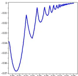
Define c(kn, km) the coefficient of|1ih1|for the combination (159). Figures 1 and 2 show that there is always a negative c(kn, km) for q∈[12,1).
Figure 1: Quantitiesc(kn, km) vsq. In particular, in the range [1/2,1/
√
2] it is plottedc(k4,−k2).
In the range [1/√2,1/2 +√3/6) it is plotted c(k2,−k1), according to Proposition 21. Finally, in
the range [1/2 +√3/6,0.8] it is plottedc(−k4, k2). In the pointq = 1/2 +
√
3/6, it isc(k2,−k1) = 0
while c(−k4, k2) =−0.0303.
A.2 Case q >1
The U(q) corresponding to (34) turns out to be
U(q) =eiarccosh √
q(ˆa†ˆb†+ˆaˆb). (160) Using the disentangling formula for theSU(1,1) group, it is possible to rewrite it as
U(q)=eraˆ†ˆb†e−s(aˆ†aˆ+ˆbˆb†)erˆaˆb, (161) where r =i r q−1 q , s= ln √ q. (162)
Let us now compute the action of U(q) on the Fock state |m1i. It results
U(q)|m1i = eˆa†ˆb†re−(aˆ†ˆa+ˆbˆb†)s ∞ X n=0 rnaˆˆbn n! |m1i (163) = eˆa†ˆb†re−(aˆ†ˆa+ˆbˆb†)s |m1i+√mr|(m−1)0i (164) = eˆa†ˆb†r ∞ X n=0 (−1)nsn ˆ a†aˆ+ ˆbˆb† n n! |m1i+ √ mr|(m−1)0i (165) = eˆa†ˆb†r ∞ X n=0 (−1)nsn(m+ 2)n n! |m1i+ √ mr ∞ X n=0 (−1)nsn(m−1 + 1)n n! |(m−1)0i ! (166) = eˆa†ˆb†r e−(m+2)s|m1i+√mre−ms|(m−1)0i (167) = e−(m+2)s ∞ X n=0 √ n+ 1 s n+m m rn|(n+m)(n+ 1)i +√mre−ms ∞ X n=0 s n+m−1 m−1 rn|(n+m−1)ni (168) = √mre−ms|(m−1)0i + ∞ X n=0 e−(m+2)s√n+ 1 s n+m m +√mr2e−ms s n+m m−1 ! rn|(n+m)(n+ 1)i. (169) Then, we can get
N(|mihm|) =m|r|2e−2ms|m−1ihm−1| + ∞ X n=0 e−(m+2)s√n+ 1 s n+m m −√mq−1 q e −ms s n+m m−1 !2 |r|2n|n+mihn+m|, (170)
and e N(|mihm|) =m|r|2e−2ms|0ih0| + ∞ X n=0 e−(m+2)s√n+ 1 s n+m m −√mq−1 q e −ms s n+m m−1 !2 |r|2n|n+ 1ihn+ 1|. (171)
It is known that for any completely positive map Γ and two density matrices ρ and σ, the following inequality for quantum relative entropy holds true (contractive property)
D(Γ(ρ)kΓ(σ))≤D(ρkσ). (172) By assuming the degradability condition forN, we should have
DNe(|m1ihm1|) Ne(|m2ihm2|) ≤D N(|m1ihm1|) N(|m2ihm2|) , (173)
for all m1 > m2 ∈N. From Eqs. (170) and (171), we have
D N(|m1ihm1|) N(|m2ihm2|) =m1|r|2e−2m1sln m1|r|2e−2m1s cqm 2(m1−m2−1) + ∞ X n=0 cqm1nln c q m1n cqm 2(m1−m2+n) , (174) and D e N(|m1ihm1|) Ne(|m2ihm2|) =m1|r|2e−2m1sln m1|r|2e−2m1s m2|r|2e−2m2s + ∞ X n=0 cqm1nlnc q m1n cqm2n , (175)
where, according to (170) and (171), we have defined
cqmn:= e−(m+2)s√n+ 1 s n+m m −√mq−1 q e −ms s n+m m−1 !2 |r|2n. (176)
By simple calculations, we get
cqmn:= (n+ 1−m(q−1)) 2 (n+ 1)qm+2 n+m m q−1 q n . (177)
Then, Eq. (173) reads
m1|r|2e−2m1sln m1|r|2e−2m1s m2|r|2e−2m2s + ∞ X n=0 cqm1nlnc q m1n cqm2n ≤m1|r|2e−2m1sln m1|r|2e−2m1s cqm 2(m1−m2−1) + ∞ X n=0 cqm1nln c q m1n cqm 2(m1−m2+n) , (178) or more simply m1|r|2e−2m1sln m2|r|2e−2m2s cqm 2(m1−m2−1) + ∞ X n=0 cqm1nln c q m2n cqm 2(m1−m2+n) ≥0. (179)
However this inequality can be violated. In fact, it happens that cqm2n= 0 when
n=m(q−1)−1. (180)
It is then clear that (179) may be violated when q is close to integer numbers. More precisely the following result holds true.
Theorem 23 For an arbitraryq >1, there exist integersm1 > m2 such that Eq.(179)is not true.
Proof Let us consider a fixed rational numberq = xy >1. By selectingm2 =y andn0=x−y−1,
we have
n0 =m2(q−1)−1, (181)
that, from (177), guaranteescqm
2n0 = 0. On the other hand, if there existsn
00such thatcq
m2(n00+m1−m2)=
0 for such q, then we should have
n00+m1−m2+ 1 m2 =q−1 ⇒ n 00+m 1−m2+ 1 y = x−y y . (182)
We choose m1 such thatm1−y 6=x−y−n00−1 for any integer n00 = 0,1, . . . , in order to have
cqm 2(n00+m1−m2)= 0. We also havec q m1n0 6= 0 to ensure that cqm 1n0ln cqm 2n0 cqm 2(m1−m2+n0) =−∞, (183)
By considering the above descriptions, we show that relation (179) violates for given small radius
ε > 0 and q < q0 < q+ε. In other words, it is clear that cmq02n 6= 0, ∀ n
1 and so we have the
condition supp(N(|m1ihm1|))⊆supp(N(|m2ihm2|)). Now, for each n≥m2(q−1) +m1, we have
cqm02n cqm0 2(m1−m2+n) = (n+1−m2(q0−1))2 (n+1)q0m2+2 n+m2 m2 q0−1 q0 n (n+m1−m2+1−m2(q0−1))2 (n+m1−m2+1)q0m2+2 n+m1−m2+m2 m2 q0−1 q0 n+m1−m2 (186) ≤ (n+1−m2(q0−1))2 (n+1) n+m2 m2 (n+m1−m2+1−m2(q0−1))2 (n+m1−m2+1) n+m1 m2 q0−1 q0 m1−m2 (187) ≤ c q m2n cqm 2(m1−m2+n) q−1 q q0−1 q0 !m1−m2 (188) ≤ c q m2n cqm 2(m1−m2+n) . (189) 1
This holds true forq0irrational number. Ifq0 is a rational number such thatcqm2n= 0, we should have
k+ 1
m2
=q0−1. (184)
On the other hand, we have|q−q0| ≤εand hence
|q−q0| ≤ε⇒ x m2 −k+ 1 +m2 m2 ≤ε, (185)
The 188 derives from n+ 1−m2(q0−1) n+m1−m2+ 1−m2(q0−1) ≤ n+ 1−m2(q−1) n+m1−m2+ 1−m2(q−1) , (190)
taking into account that n≥m2(q−1) +m1.
On the other hand, we have lim n→∞ cqm2n cqm 2(m1−m2+n) = 1 |r|2m1 = q q−1 m1−m2 . (191)
Therefore, for a given η >0 the exists a number Nη such that for anyn≥Nη ≥m2(q−1) +m1,
it is cqm2n cqm 2(m1−m2+n) ≤ q q−1 m1−m2 +η. (192)
It then follows, using (179) and the fact Tr(N(|m1ihm1|)) = 1, that
∞ X n=Nη cqm1nln c q m2n cqm 2(m1−m2+n) ≤ln ( q q−1 m1−m2 +η ) ∞ X n=0 cm1n≤ln ( q q−1 m1−m2 +η ) . (193) Using relations (189) and (193), we can get
∞ X n=Nη cqm01nln c q0 m2n cqm0 2(m1−m2+n) ≤ ∞ X n=Nη cqm01nln c q m2n cqm 2(m1−m2+n) (194) ≤ ∞ X n=Nη cqm01nln c q m2n cqm 2(m1−m2+n) (195) ≤ ln ( q q−1 m1−m2 +η ) ∞ X n=Nη cqm01n (196) ≤ ln ( q q−1 m1−m2 +η ) . (197)
Finally, we find that Eq. (179) holds for q0≤Θ1+ Θ2, where
Θ1 ≡m1|r|2e−2m1sln m2|r|2e−2m2s cqm0 2(m1−m2−1) + Nη−1 X n=0,n6=n0 cqm01nln c q0 m2n cqm0 2(m1−m2+n) + ln ( q q−1 m1−m2 +η ) , (198) Θ2 ≡cq 0 m1n0ln cqm0 2n0 cqm0 2(m1−m2+n0) . (199)
Now, whenεgoes to 0, the quantity Θ1 will remain finite (it is continuous with respect toq), while
the quantity Θ2 diverges to−∞. Therefore, for any rational number q we can find a set (q, q+),
for q0, which violates (179). Since the set of rational numbers is dense into the set of reals, the proof follows.
B
Bounds on capacities uncertainty
In this appendix we derive, on the basis of relations (107) and (108), tighter lower bounds on the sum χH⊗+χA⊗ than the one from Theorem 14 for one-mode Gaussian channels. The reasoning
is based on the classification of OMG channels given in [13], and the bounds are derived by using coherent states encoding.
• Class A1: M = 0, N N>=I. We have χH⊗≥S 1 2I −S 1 2I = 0, (200) and χA⊗≥S PE+ 1 2 I −S 1 2I ≥g PE+ 1 2 . (201) Therefore, we get χH⊗+χA⊗≥g PE+ 1 2 . (202) • Class A2: M = 1 0 0 0 ,N N>=I. We have χH⊗≥S PA+ 1 0 0 12 −S 1 0 0 12 , (203) and χA⊗ ≥S PE+ 1 0 0 PE +12 −S 1 0 0 12 . (204) Therefore, we get χH⊗+χA⊗≥g r (PA+ 1) 1 2 ! +g s (PE+ 1) PE+ 1 2 ! −2g r 1 2 ! . (205) • Class B1: M =I,N N>= 2N1 0+1 1 0 0 0 . We have χH⊗≥S PA+12 +2N10+1 0 0 PA+12 −S 1 2 + 1 4N0+2 0 0 12 , (206) and χA⊗≥S PE+12 2N0+1 + 1 2 0 0 12 !! −S 1 2 + 1 4N0+2 0 0 12 . (207)
Therefore, we get χH⊗+χA⊗≥g s PA+ 1 2 + 1 2N0+ 1 PA+ 1 2 ! +g s PE+12 4N0+ 2 +1 2 −2g r 1 4+ 1 4N0+ 2 . (208) • Class B2: M =I,N N>= N0 N0+12I. We have χH⊗≥S PA+ 1 2+ N0 2N0+ 1 I −S 1 2 + N0 2N0+ 1 I , (209) and χA⊗ ≥S (PE +12)N0 N0+ 12 +1 2 ! I ! −S 1 2+ N0 2N0+ 1 I . (210) Therefore, we get χH⊗+χA⊗ ≥g PA+ 1 2 + N0 2N0+ 1 +g (PE + 1 2)N0 N0+12 +1 2 ! −2g 1 2 + N0 2N0+ 1 . (211) • Class C Att: M =√κI,N>N = (1−κ)I, 0< κ <1 We have χH⊗≥S PA+ 1 2 κ+ 1−κ I −S 1 2I , (212) and χA⊗≥S PE+ 1 2 (1−κ) +κ I −S 1 2I . (213) Therefore, we get χH⊗+χA⊗≥g PA+ 1 2 κ+ 1−κ +g PE+ 1 2 (1−κ) +κ . (214)
• Class C Amp: M =√κI,N N>= (κ−1)I, forκ >1. We have χH⊗≥S PA+ 1 2 κ+κ−1 I −S κ−1 2 I , (215) and χA⊗≥S PE+ 1 2 (κ−1) +κ I −S κ−1 2 I . (216)
Therefore, we get χH⊗+χA⊗≥g PA+ 1 2 κ+κ−1 +g PE + 1 2 (κ−1) +κ −2g κ−1 2 . (217) • Class D:M =√−κZ,N>N = (1−κ)I,κ∈(−∞,0) We have χH⊗≥S PA+ 1 2 |κ|+|1−κ| I −S |κ|+|1−κ| 2 I . (218) and χA⊗≥S PE + 1 2 (|1−κ|) +|κ| I −S | κ|+|1−κ| 2 I . (219) Therefore, we obtain χH⊗+χA⊗≥g PA+ 1 2 |κ|+ 1−κ +g PE+ 1 2 (1−κ) +|κ| −2g | κ|+|1−κ| 2 . (220)
Remark 24 For an easy comparison with the bound in Theorem 14, let us consider the class C. The r.h.s. of (214) and (217) can be put together as
g PA+ 1 2 κ+|1−κ| +g PE + 1 2 |1−κ|+κ −2g |1−κ|+κ 2 . (221)
Due to the properties of the functiong defined in (23), it is
Eq.(221)≥g min{PA, PE}+ 1 2 κ+|1−κ| +g min{PA, PE}+ 1 2 |1−κ|+κ −2g | 1−κ|+κ 2 . (222)
Still referring to the properties of the function g, we have that the quantity (222) grows, in terms of min{PA, PE}, faster than (99). Thus, the minimum difference between the two bounds ((221)
and (99)) is achieved when min{PA, PE} goes to zero and results at least as much big as
g 1−1 2κ +g 1 +κ 2 , κ <1 (223) 2g 3 2κ−1 −2g κ− 1 2 , κ >1. (224)