WORKING PAPER NO. 10-1
INSURING COLLEGE FAILURE RISK
Satyajit Chatterjee
Federal Reserve Bank of Philadelphia
and
Felicia Ionescu
Colgate University
Insuring College Failure Risk
∗
Satyajit Chatterjee
†Federal Reserve Bank of Philadelphia
Felicia Ionescu
‡Colgate University
November 2009
Abstract
Participants in student loan programs must repay loans in full regardless of whether they complete college. But many students who take out a loan do not earn a degree (the dropout rate among college students is between 33 to 50 percent). We examine whether insurance against college-failure risk can be offered, taking into account moral hazard and adverse selection. To do so, we develop a model that accounts for college enrollment, dropout, and completion rates among new high school graduates in the US and use that model to study the feasibility and optimality of offering insurance against college failure risk. We find that optimal insurance raises the enrollment rate by 3.5 percent, the fraction acquiring a degree by 3.8 percent and welfare by 2.7 percent. These effects are more pronounced for students with low scholastic ability (the ones with high failure probability).
Keywords: College Risk; Government Student Loans; Optimal Insurance JEL Codes: D82; D86; I22;
1
Introduction
Recent research in the education literature provides support for the fact that financial constraints during college-going years are not crucial for college enrollment (Carneiro and Heckman (2002), Cameron and Taber (2001)). Rather, it is student characteristics, such as learning ability, that determine the decision to enroll.
∗The authors thank Orazio Attanasio, Lutz Hendricks, Narayana Kocherlakota, Luigi Pistaferri, Victor Rios-Rull, and
Viktor Tsyrennikov for helpful comments and Matt Luzzetti for excellent research assistance. Comments from participants at the NBER-EFACR group, the Society of Economics Dynamics, Econometrics Society and Midwest Macroeconomic Meetings and seminar participants at Cornell University and the University of Connecticut are also gratefully acknowledged. The views expressed here are those of the authors and do not necessarily represent the views of the Federal Reserve Bank of Philadelphia or the Federal Reserve System. This paper is available free of charge at www.philadelphiafed.org/research-and-data/publications/working-papers/.
†Federal Reserve Bank of Philadelphia, Ten Independence Mall, Philadelphia PA, 19106; (215)574-3861,
Given the generosity of the student loan program, funds are readily available and eligible high school gradu-ates invest in college if they perceive the returns to a college education to be high enough (Ionescu (2009a)).1
However, there is considerable financial risk in taking out a student loan because many students do not complete college. Using the 1990 Panel Study of Income Dynamics (PSID), Restuccia and Urrutia (2004) document that 50 percent of people who enroll do not complete college. Using the NCES data and surveys, we find that 37 percent and 35 percent of students enrolled in 1989-90 and 1995-96, respectively, do not possess a degree and are not enrolled in college five years after their initial enrollment.
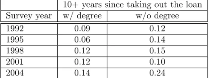
The financial risk implied by these facts is evident in the Survey of Consumer Finances (SCF). For the five surveys conducted between 1992 and 2004, the percentage of non-students with a student loan who report not having either a 2- or 4-year college degree is 47 percent, on average. Furthermore, non-students with loans but without a degree have a significantly higher (education) debt burden. Table 1 reports the ratio of median education debt to median income among non-students with student loans, 10 or more years after first taking out the loan. As is evident, students without degrees have a significantly higher debt burden than degree holders.
Table 1: College debt burden by completion status
10+ years since taking out the loan Survey year w/ degree w/o degree
1992 0.09 0.12
1995 0.06 0.14
1998 0.12 0.15
2001 0.12 0.10
2004 0.14 0.24
The financial risk of taking out a student loan but being unable to complete college may discourage some people from taking out a loan and enrolling in college. Thus, even though prospective students may not be credit constrained, a mechanism to share the risk of failing to complete college –college failure risk – might improve the welfare of enrolled students and encourage more people to enroll and complete college.2
The aim of this paper is to study whether the student loan program can offer insurance against college failure risk. The current operation of the program suggests that it is administratively feasible to offer some
1For detailed evidence on how financial aid affects students’ college-going behavior, see Dynarski (2003) and Hoxby (2004).
The former study presents evidence that financial factors represent an important determinant of both enrollment and persistence. The latter provides a comprehensive perspective on the issue of college choice, examining it from both an individual and institutional point of view. Also, for an extensive analysis of the college financial system’s weaknesses and strengths, see Kane (1999).
2Heckman (1999) has pointed out that the erosion of average real wages between 1980 and 1990 could have been mitigated
(in an accounting sense) if more people had acquired college degrees. Specifically, for the 1990 workforce of 120 million, 5.4 million more would have to become college equivalents to reverse the 1980-1990 erosion of real wages, and about 1 million additional skilled persons would need to be added to the workforce each year on top of the once and for all change of 5.4 million.
insurance. Under the current system, a borrower can choose from a menu of fairly sophisticated repayment options (standard, graduated, income-contingent and extended repayment). Nevertheless, under each of these payment options, the borrower is required to repay the entire loan and associated interest expenses regardless of whether he or she completed college. We will examine whether it is feasible to forgive a portion of the loan for students who fail out of college.3
We conduct our investigation under two important constraints on the provision of failure insurance. First, we require that the insurance scheme not distribute resources from people with a high probability of completion to people with a low probability of completion (and vice versa). Formally, this requires that the insurance program be self-financing with respect to each person who chooses to participate. The current programs enforce this self-financing constraint regardless of whether the program participant actually graduates from college. We will permit failures to pay less than graduates, but each participant will pay the full cost of college in expectation. Second, we require that the insurance program guard against adverse selection (the possibility that poor risks will attempt to pool with good risks). As we verify later, moral hazard is not an issue in this context because insurance against college failure risk increases the value of exerting effort in college.
In the theoretical section of the paper, we develop a simple model of a student’s enrollment and college effort decisions. The model postulates the necessary heterogeneity in student characteristics in order to be consistent with the diversity of enrollment and effort decisions we see in reality and the importance generally assigned to ability heterogeneity and self-selection into college attendance and completion by researchers (see, for instance, Venti and Wise (1983)). The heterogeneity is in a student’s utility cost of putting effort into college and his or her outside option, neither of which is directly observable to loan administrators. The unobserved heterogeneity complicates the task of providing insurance. These complications are analyzed in the theoretical section and the constrained optimization problem that delivers the optimal insurance program is developed.
In the quantitative section, we calibrate the model to US data on college enrollment, leaving, and completion rates as well as the average college costs of program participants, distinguishing between students of different scholastic ability levels as measured by SAT scores. We quantify the effects of insurance on enrollment and completion rates as well as welfare. The optimal insurance offered in case of non-completion ranges between 10 to 45 percent of total college cost. The insurance scheme induces an increase in the enrollment rate of 3.5 percentage points and an increase in college graduates of 3.8 percentage points. Although insurance draws in students with a high risk of failure, completion rates rise because fewer students voluntarily leave college. Insurance increases welfare by 2.7 percent on average.
There is a rich literature on higher education, with important contributions focusing on college enrollment and completion. Studies that take a quantitative-theoretical approach have given a prominent role to the risk of college failure. These include studies by Akyol and Athreya (2005); Caucutt and Kumar (2003); Garriga and Keightley (2007); Ionescu (2009b); Restuccia and Urrutia (2004). But these studies do not generally consider the possibility of providing insurance against this risk. One exception is Ionescu (2009b) who studied the effects of alternative bankruptcy regimes for student loans. She shows that individuals with relatively low ability and low initial human capital levels are affected to a greater degree by the risk of failure and the option to discharge one’s debt under a liquidation regime helps alleviate some of this risk.4 Also,
with the exception of Garriga and Keightley (2007) none of these studies recognize that students may choose to drop out.5
Empirical research on college behavior, however, calls for a careful modeling of college dropout behavior. Manski and Wise (1983) argue that college students learn over time about what college means and given this learning some choose to drop out. In addition, they suggest that college preparedness is more important than college aspiration for college completion. Furthermore, Stinebrickner and Stinebrickner (2008) show that most of the attrition among students from low-income families cannot be attributed to short-term credit constraints.6 In a companion paper, Stinebrickner and Stinebrickner (2009) provide evidence on the relative
importance of the most prominent alternative explanations for dropout behavior and find that learning about ability plays a particularly important role in this decision. Among other possible factors of importance, they find that students who find school to be unenjoyable are unconditionally much more likely to leave. But this effect seems to arise to a large extent because these same students also tend to receive poor grades. In our model, dropout behavior will arise for similar reasons.
Our paper is related to studies that focus on merit-based policies. Our insurance arrangement can be interpreted as being merit based: as we show later in the paper, the insurance premium is lower for higher ability types and the amount of insurance offered is higher as well. However, unlike merit-based aid, our insurance arrangement has no aid or grant component – it is self-financed with respect to each individual who participates, in expectation. Caucutt and Kumar (2003) analyze various types of college subsidies and conclude that merit-based aid that uses any available signal on ability increases educational efficiency with little decrease in welfare. Gallipoli, Meghir, and Violante (2008) examine the partial and general equilibrium effects of wealth-based and merit-based tuition subsidies on the distribution of education and earnings. In
4Although insurance against college failure risk is not the focus of their paper, Akyol and Athreya (2005) observe that the
heavy subsidization of higher education directly mitigates the risk of college failure by reducing the college premium.
5Garriga and Keightley (2007) model college as a multi-period risky investment with endogenous enrollment, time-to-degree,
and dropout behavior. The focus of their paper is on the effects of broad-based tuition subsidies and merit-based education policies on college enrollment and completion behavior rather than insurance against college failure risk.
6The authors use unique longitudinal data that have been collected specifically for this type of purpose at Berea College.
Despite the fact that the direct costs to students at Berea are approximately zero, the authors document that 50 percent of students do not graduate.
related work, Redmon and Tamura (2007) use a Mincer model of human capital with ability differences to characterize the optimal length of schooling by ability class and the importance of school district composition for growth and distribution.
The key contribution of this paper is to construct a theory consistent with the reality of college enrollment, leaving and completion behavior as well as returns to education and use it to design an insurance scheme against the risk of failing at college, recognizing adverse selection and moral hazard. In addition, we map the model to the data and quantify the effects of alternative insurance arrangements on enrollment, completion and welfare. The rest of the paper is organized as follows. Section 2 presents the choices available to a student. Section 3 lays out the key predictions of this model when no insurance is offered and compares these predictions to patterns in the data. Section 4 develops the constrained optimization problem that delivers the optimal insurance scheme. Parameter selection and calibration of the model are presented in Section 5. Section 6 presents the results of offering insurance in the calibrated model and Section 7 concludes.
2
Environment
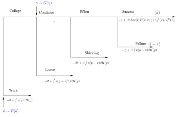
Time is discrete and indexed byt={0,1,2, . . .}.In period 0,a prospective student makes a one-time decision to enroll in college or not. If she does not enroll, she can work in a low-paid job with disutility of effortθ≥0 and, starting in period 1, earn y ≥0. The earnings y are drawn from a distribution H(y). At the time of the enrollment decision, the student knowsθbut not the realization ofy.
If the individual chooses to enroll in college, she learns the cost of making effort in college. Effort, e, is a binary variable that can take values 0 (no effort) or 1 (effort).7 The cost of making an effort is denotedγ
and the student draws γ ≥0 from a distributionG(γ). After she learns γ the student decides whether to continue on in college. If she chooses to leave, she incurs the cost of effortθ in the low-paid job and draws her (life-time) earningsy in period 1. She also incurs some partial college expenses φx, where 0< φ <1.8
At the time of choosing whether to continue in college, the student knowsγ and θbut not her earnings in period 1 and beyond.
If the student continues in college she incurs the annual college cost ofx. A continuing student must choose between putting in effort or not. If she chooses to shirk (e= 0), she will fail with probability 1 but she will not incur effort costs of any kind in period 0 and will start life in period 1 with an earnings drawyfrom the distributionH(y) and a debt ofx.If she chooses to put in effort (e= 1), she will complete her first year with
7The assumption that effort is binary is essentially without loss of generality. Given the large college premium in earnings
it is safe to assume that if a student finds it optimal to exert any effort in college, he or she would want to exert the maximum effort possible.
8We assume that if a student voluntarily withdraws from college, he or she pays a cost that is some (relatively small)
Figure 1: Timing of decisions
probability π∈(0,1). If she completes successfully, she begins period 1 as a college student with one more year to go and debt ofx(no interest accumulates on the debt as long as the student continues in college). If she fails to complete, she starts period 1 with an earnings drawy from H(y) and a debt ofx.
Figure 1 illustrates this timing of period 0 decisions. In the case in which a student succeeds in completing the first year of college, she faces a similar decision tree in period 1 (which we will describe below).
In period 1,a student with one more year to go has to choose again whether to continue in college. If she does not continue, she gets an earnings drawyfrom the distributionH(y) and starts her life with debt 5x/4. If she continues, she incurs another year of college expensex. And, as in period 0,she must choose between putting in effort or shirking. If she shirks, she fails with probability 1 but does not incur any effort cost in period 1 and starts life in period 2 with an earnings draw y from the distribution H(y) and a debt of 2x.
If she puts in effort, she completes college with probabilityπ. If she succeeds in completing, she draws her life-time earningsyfrom the distributionM(y) and has debt of 2x. If she fails to complete college, she starts period 2 with an earnings drawyfrom H(y) and a debt of 2x.
In order to describe individuals’ decision problems in period 0 and 1 (these are the only periods in which there are decisions to be made), we will start with describing the utility (payoffs) to students at the start of
period 1 (students that have one more year of college to go).
1. A student who drops out gets
V1D(x) = ˆ
U(y−5x/4)dH(y).
2. A student who continues but shirks gets
V1S(x) =β
ˆ
U(y−2x)dH(y).
3. A student who continues and puts in effort gets
V1E(π, x, γ) =−γ+β π ˆ U(y−2x)dM(y) + (1−π) ˆ U(y−2x)dH(y) .
Turning to period 0,the payoffs are as follows
1. An individuals who does not enroll gets
W(θ) =−θ+β
ˆ
U(y)dH(y).
2. An individual who enrolls, but drops out gets
V0D(x, θ) =−θ+
ˆ
U(y−x/4)dH(y).
3. An individual who enrolls, continues and shirks gets
V0S(x, θ) =−βθ+β
ˆ
U(y−x)dH(y).
4. An individual who enrolls, continues and puts in the effort gets
V0E(π, x, γ) =−γ+β πmax[V1E(π, x, γ), V1S(x), V1D(x)] + (1−π) ˆ U(yN−x)dH(yN) .
The structure of payoffs is generally self-explanatory. One aspect worth remarking on is that leaving or shirking in period 0 forces the individual to work in the low-paid job for 1 period. In contrast, if the student fails in period 0 despite putting in effort, she does not have to work in the low-paid job. This assumption
is a convenient way to capture the fact that exerting effort in college has benefits even if it does not lead to college credits. Also, since anyone who is in college in period 1 must have successfully completed one year of college (and therefore exerted effort in period 0), she can drop out or shirk and not have to work in the low-paid job. Thus,θ does not appear in eitherVD
1 (x) orV1S(x).
We make the following set of assumptions on the primitives.
Assumption 1: U(c) :R→R++ withU0(·)>0 andU00(·)<0.
Assumption 2: β2´U(y−2x)dM(y)>´U(y)dH(y) (college degree is profitable financial investment).
Assumption 3: ´z(y)dM(y) > ´z(y)dH(y) for any z(y) strictly increasing in y (the distribution M
first-order stochastic dominates the distributionH).
3
College Enrollment, Dropout and Failure Under the Current System
We begin by studying the choice problem in period 1. There are three options open to the student. She could drop out, or continue on in college but not put in any effort, or she could continue on in college and exert effort.
Proposition 3.1. In period 1, there is a cut-off γ1(x, π)≥0 such that forγ > γ1(x, π), students drop out
and forγ≤γ1(x, π)they continue on with effort. Furthermore,γ1(x, π)is increasing in π.
Proof. Since 5x/4 <2xand β < 1,V1D(x) > V1S(x). Hence, dropping out is strictly better than shirking
in period 1. Therefore, the student chooses between continuing on with effort or dropping out. Denote the difference in payoffs between these two choices byV1(x, π, γ) =V1E(x, π, γ)−V1D(x). Observe thatV1(x, π, γ)
is continuous and strictly decreasing inγ∈[0,∞). IfV1(x, π,0)≤0, thenγ1(x, π) = 0. IfV1(x, π,0)>0, by
continuity and strict monotonicity with respect toγ, there exists a unique ˆγ >0 such thatV1(x, π,γˆ) = 0.
Henceγ1(x, π)>0.
To proveγ(x, π) is increasing inπnote that
V1(x, π, γ) = −γ+βπ ˆ U(y−2x)dM(y)− ˆ U(y−2x)dH(y) +β ˆ U(y−2x)dH(y)− ˆ U(y−x)dH(y).
By Assumption 2,V1(x, π, γ) is strictly increasing inπ. Now consider ˆπ <π˜. IfV1(x,π,ˆ 0)< V1(x,π,˜ 0)≤0,
then γ1(x,πˆ) = γ1(x,π˜) = 0. If V1(x,ˆπ,0) ≤ 0 < V1(x,π,˜ 0), then 0 = γ(x,πˆ) < γ(x,π˜). Finally, if
0< V1(x,π,ˆ 0)< V1(x,π,˜ 0),then 0< γ(x,πˆ)< γ(x,˜π). This establishes thatγ(x, π) is increasing inπ.
It is perhaps worth noting that the threshold γ will be zero for sufficiently low probability of success π. Observe thatV1(x,0,0)<0 and, by Assumption 2,V1(x,1,0)>0. Thus, when no effort in school is required
(γ= 0) there existsπ1>0 such thatV1(x, π1,0) = 0.For allπ < π1,V1E(x, π, γ)−V
D
1 (x)<0 for allγ≥0.
Therefore, the thresholdγ1(x, π) is 0 for allπ≤π1.
We now study the choices in period 0. The choice problem can be broken down into two parts. First, conditional on not putting in effort in college, is it better to drop out or shirk? And, second, given the answer to the first question, is it better to put in effort in college?
Proposition 3.2. In period 0, there exists a cut-off θ0(x)>0 such that conditional on not putting in effort
in college students drop out forθ < θ0(x)and shirk for θ≥θ0(x).
Proof. Consider the functionVD
0 (x, θ)−V0S(x, θ) =−θ(1−β) +
´
U(y−x/4)dH(y)−β´ U(y−x)dH(y), which is continuous and strictly decreasing inθ∈[0,∞). We haveVD
0 (x,0)−V0S(x,0) =
´
U(y−x/4)dH(y)− β´U(y−x)dH(y) > 0. By continuity and strict monotonicity with respect to θ, there exists θ0(x) > 0
such thatVD
0 (x, θ0(x))−V0S(x, θ0(x)) = 0.For anyθbelow this cut-off, dropping out is strictly preferred to
shirking and at or above this cut-off, shirking is weakly or strictly preferred to dropping out.
Proposition 3.2 shows that conditional on not putting in effort in college, some students would rather spend time in college shirking than dropping out so as to delay paying the costθ. Students who choose to do this are using the student loan program to borrow and consume leisure.
The next proposition deals with the decision to put in effort in college in period 0.
Proposition 3.3. In period 0, there exists a cut-offγ0(x, π, θ)≥0such that forγ < γ0(x, π, θ)(if applicable),
students put in effort in period 0 and forγ≥γ0(x, π, θ)they either drop out or shirk. Furthermore,γ0(x, π, θ)
is increasing in πandθ.
Proof. Consider the functionV0(x, π, γ, θ) =V0E(x, π, γ)−max[V0D(x, θ), V0S(x, θ)] which is continuous for
all (π, γ, θ)∈[0,1]×[0,∞)×[0,∞) and strictly increasing in π (by Assumption 2), strictly decreasing in
γ and strictly increasing in θ. IfV0(x, π,0, θ)≤0, then γ0(x, π, θ) = 0. If V0(x, π,0, θ)>0, by continuity
and strict monotonicity with respect to γ there exists a unique ˆγ > 0 such that V0(x, π,γ, θˆ ) = 0. Thus,
The fact that γ0(x, π, θ) is increasing inπ can be established exactly along the lines of the proof given in
Proposition 3.1.
To proveγ0(x, π, θ) is increasing inθ, consider ˜θ <θˆ. IfV0(x, π, γ,θ˜)< V0(x, π, γ,θˆ)≤0, thenγ0(x, π,θ˜) =
γ0(x, π,θˆ) = 0. If V0(x, π, γ,θ˜) ≤ 0 < V0(x, π, γ,θˆ), then 0 = γ0(x, π,θ˜) < γ0(x, π,θˆ). Finally, if 0 <
V0(x, π, γ,θ˜)< V0(x, π, γ,θˆ) then 0< γ0(x, π,θ˜)< γ0(x, π,θˆ). This establishes thatγ0(x, π, θ) is increasing
inθ.
These propositions can be conveniently seen in Figure 2. The left (right) figure presents the choices that the student makes in period 0 (period 1) in terms of the effort levels required on the job,θ, and the effort level required in college,γ.
Figure 2: Choices in periods 0 and 1
Propositions 3.1 and 3.3 give us two thresholds forγ. It is important to understand the relationship between them because it will play an important role in the discussion of optimal insurance. We have the following proposition.
Proposition 3.4. Assume that π > π¯1. For sufficiently low value of θ, γ0(x, π, θ) < γ1(x, π) and for
sufficiently high value ofθ,γ0(x, π, θ)> γ1(x, π).
Proof. We will evaluate V0(x, π, γ, θ) at the value of γ for which the student is indifferent between putting
in effort or dropping out in period 1.
Forπ >π¯1andθ < θ0(x),V0(x, π, γ1(x, π), θ) =−γ1(π, x) +θ−β[
´
U(y−x/4)dH(y)−´U(y−x)dH(y)]− βπ[´ U(y−x)dH(y)−´ U(y−5x/4)dH(y)].This implies that forθsufficiently close to 0,V0(x, π, γ1(x, π), θ)<
0. Hence, forθsufficiently small,γ0(x, π, θ)< γ1(x, π).
Forπ >π¯1andθ > θ0(x),V0(x, π, γ1(x, π), θ) =−γ1(π, x)+βθ−βπ[
´
U(y−x)dH(y)−´U(y−5x/4)dH(y)]. This implies that forθ sufficiently large V0(x, π, γ1(x, π), θ)>0. Hence forθ sufficiently large,γ0(x, π, θ)>
The significance of these results is that for a student with γ < γ0(x, π, θ)< γ1(x, π) it is optimal to put in
effort in period 0, and if she successfully completes college in period 0, to also put in effort in period 1. In contrast, for a student withγ1(x, π)< γ < γ0(x, π, θ), it is optimal to put in effort in the first year of college
but then drop out even if he or she is successful. This is a student for whom the cost of effort is high enough that exerting effort throughout both years of college is not optimal but it is low enough (and disutility from the low-paid job high enough) that it is optimal to exert effort in the first year of college and thereby avoid
θ.
Next we will determine who enrolls in college. Observe that since enrolling in college and then leaving gives people about the same utility as working, there is a small cost to a student to enroll in college and learn her
γ. However, if the student’s probability of success is sufficiently low, she may choose not to enroll because regardless of the value ofγshe will find it optimal to leave rather than continue with college. Similarly, for a student of a given probability of success, if the effort in the low-paid job is sufficiently high, she may choose to enroll.
The following proposition gives the cut-off value of effort required on the job that makes the student indifferent between working and enrolling in college. For every effort less than that, the student strictly prefers not to enroll.
Proposition 3.5. In period 0, there exists a cut-off θC(x, π)≥0 such that for θ > θC(x, π) enrolling gives
at least as much utility as working and θ ≤ θC(x, π) working gives at least as much utility as enrolling.
Furthermore, θC(x, π)is decreasing inπ.
Proof. Consider the function VC(x, π, θ) =´ max{VE
0 (x, π, γ), V0D(x, θ), V0S(x, θ)}dG(γ)−W(θ). We will
show that this function is increasing inθ. Observe that
VC(x, π, θ) = ˆ γ0(x,π,θ) 0 V0E(x, π, γ)dG(γ) + ˆ γ0(x,π,θ) max[V0D(x, θ), V0S(x, θ)]dG(γ)−W(θ).
Letθincrease by ∆>0. Consider the effect of this change onVC(x, π, θ) in 2 parts:
VC(x, π, θ+ ∆)−VC(x, π, θ) = [VC(x, π, θ+ ∆)−VC¯ (x, π, θ+ ∆)] + [ ¯VC(x, π, θ+ ∆)−VC(x, π, θ)]. where ¯ VC(x, π, θ+∆) = ˆ γ0(x,π,θ) 0 V0E(x, π, γ)dG(γ)+ ˆ γ0(x,π,θ) max[V0D(x, θ+∆), V0S(x, θ+∆)]dG(γ)−W(θ+∆).
Then [ ¯VC(x, π, θ+ ∆)−[VC(x, π, θ)] is given by ˆ γ0(x,π,θ) max{−(θ+ ∆) + ˆ u(y−x/4)H(dy),−(θ+ ∆)β+β ˆ u(y−x)H(dy)}dG(γ)} − ˆ γ0(x,π,θ) max{−θ+ ˆ u(y−x/4)H(dy),−θβ+β ˆ u(y−x)H(dy)}dG(γ)} +∆
Observe that the above change is non-negative because the positive ∆term contributes ∆ while the negative ∆ term contributes either -∆G(γ0(x, π, θ)) (in the case whereθ+ ∆< θ0) or−β∆G(γ0(x, π, θ)) (in the case
whereθ+ ∆≥θ0). Furthermore, the term [VC(x, π, θ+ ∆)−VC¯ (x, π, θ+ ∆)] is non-negative by optimality.
Hence,VC(x, π, θ+ ∆)−VC(x, π, θ)≥0. ThusVC(x, π, θ) is increasing inθ.
SinceVC(x, π, θ) is increasing inθ,if enrolling is optimal for someθ,enrolling must also be optimal for any
ˆ
θ greater than θ. Therefore, there must be a cut-off valueθC(x, π)≥0 such that for all θ > θC(x, π) the
student will find it optimal to enroll and forθ≤θC(x, π) the student will find it optimal to not enroll.
To establish that the threshold is decreasing in π observe thatVE
0 (x, π, γ) is strictly increasing in π and,
therefore,VC(x, π, θ) is strictly increasing inπ. It follows that the cut-offθC(x, π) cannot be strictly increasing inπ.
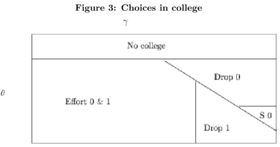
Our model of college enrollment and college completion is consistent with a diversity of student behavior. First, it predicts that not every student will enroll in college. Second, among those who enroll some will leave college voluntarily or shirk in period 0. These are the students who discover that their disutility from putting in effort in college is higher thanγ0(x, π, θ). Third, there will be students who continue on in college
(and put in effort) in period 0, but fail to complete their courses satisfactorily with probability 1−π. Fourth, among students who successfully complete their courses in period 0, some will leave college voluntarily in period 1. These are the students whose disutility from putting in effort in college happens to be between
γ0(x, θ, π) andγ1(x, π). Fifth, there will be students who continue on in college (and put in effort) in period
1, but fail to graduate, with probability 1−π. Finally there are students who enroll in college and complete their degrees. Figure 3 sums up this diversity of behavior as determined by the two types of effort costs, θ
andγ.
Next, we turn briefly to the observable implications of the theory. Among other things, the theory implies specific patterns regarding enrollment, non-completion and earnings with respect to the probability of success
π. If prospective students can be classified by some observable index of their probability of success in college conditional on putting in effort – by their scholastic ability – the theory makes predictions about the variation in student performance across scholastic ability groups. In what follows, we will assume that there is an
Figure 3: Choices in college
observable indexathat varies positively with probability of successπ. That is,
Assumption 4: π(a) is increasing ina.
We study how the cut-offs illustrated above change witha, holding all other primitives constant. The purpose is to show that the model is consistent with the basic qualitative patterns in the data regarding enrollment, non-completion and earnings across observed ability groups. As we will document in section 5, ifais proxied by SAT scores we find that enrollment rates are increasing in a, non-completion rates are decreasing in a
and earnings are increasing ina.
Proposition 3.5 delivers thatθC(x, π) is decreasing in the probability of successπ. Sinceπ(a) is increasing in
athis implies that the enrollment cut-off is declining ina. Hence, enrollment rates – defined as the fraction of students of a particular ability group who enroll in college – are increasing ina.
For each ability leveladefine thenon-completion rate,n(a),as the sum of the fraction of students who enroll in college but drop out, shirk or fail in period 0, or drop out or fail in period 1. That is,
n(a) = [1−G(γ0(x, π(a), θ)] + [1−π(a)]G(γ0(x, π(a), θ)) +π(a)G(γ0(x, π(a), θ))
×{[1−G˜(γ1(x, π(a), θ))] + [1−π(a)] ˜G(γ1(x, π(a)))},
where ˜G(γ) = min{1,G(γ0(Gx,θ,π(γ)(a)))} is the distribution ofγconditional onγ < γ0(x, π(a), θ).
Proposition 3.6. The non-completion rate n(a) is decreasing ina.
Proof. The expression for n(a) simplifies to 1−π(a)2G(γ
expression of ˜G(γ) we get n(a) = 1−π(a)2G(γ0(x, θ, π(a))) min 1, G(γ1(x, π(a))) G(γ0(x, θ, π(a))) = 1−π(a)2min{G(γ0(x, θ, π(a))), G(γ1(x, π(a)))}
The result follows from Propositions 3.3 and 3.1, which established thatγ0(x, π, θ) andγ1(x, π) are increasing
inπand the assumption thatπ(a) is increasing ina.
Next we show that average earnings are increasing in scholastic ability. By average earnings of a scholastic groupawe mean e(a) =F(θC(x, π(a))) ˆ ydH(y) + [1−F(θC(x, π(a)))][n(a) ˆ ydH(y) + (1−n(a)) ˆ ydM(y)]
Proposition 3.7. Average earningse(a)are increasing ina.
Proof. Follows from Proposition 3.5, which established thatθC(x, π) is decreasing inπand thereforeθC(x, π(a))
is decreasing inaand Proposition 3.6, which delivered thatn(a) is decreasing ina, and Assumption 3, which implies´ydM(y)>´ ydH(y).
These propositions relied on the assumption that aaffected π only. It is possible that aalso affects other primitives, for instance, the distribution from which the effort costγ is drawn, the distribution from which earningsy are drawn and the college cost 2x. Indeed, in the quantitative section, we will permitato affect these distributions and the college cost as well.
4
Insuring College Failure Risk
Can the student loan program gainfully offer insurance against college failure risk? As noted in the intro-duction, we wish to answer this question, recognizing that the student loan program cannot redistribute resources from students with a high probability of success (high ability) to students with a low probability of success (low ability) and recognizing that insurance against college failure may encourage shirking (and therefore failure).
It is best to break up the answer into two parts. Consider first the nature of optimal insurance in period 1 when loan administrators can observe effort so that moral hazard is not an issue. Conditional on the student having put in effort, the student loan program gives a transferf1to a student if she fails college and collects a
premiums1if she completes college. Since the insurance is required to be self-financing (no cross-subsidies),
we must have−π·s1+ (1−π)·f1= 0. Ignoring the−γ term, expected utility given these transfers is then
π·
ˆ
U(y−2x−[(1−π)/π]f1)dM(y) + (1−π)·
ˆ
U(y−2x+f1)dH(y).
Maximizing the above expression with respect tof1 yields the following first-order condition:
ˆ
U0(y−2x−[(1−π)/π]f1)dM(y) =
ˆ
U0(y−2x+f1)dH(y).
Hence the value of f1 that attains the maximum is one that equalizes the expected marginal utility of
consumption following failure and success. Denote this value off1byf1∗. Because there is a college premium
in earnings (meaning that the distributionM(y) first-order stochastic dominates the distribution H(y)) the value off∗
1 will typically far exceed the cost of college 2x. Henceforth, we will proceed under the assumption
that this is so.
Assumption 5: f1∗>2x(first best insurance exceeds college costs)
Since our goal is to study the possibility of offering insurance against the risk of paying for college but failing to graduate, we limit the maximum insurance that can be offered against failure to 2x. The following is then true.
Lemma 4.1. Given Assumption 5,VE
1 (x, π, γ, f1)) =−γ+β[πU(y−2x−f1π/(1−π))+(1−π)U(y−2x+f1)]
is strictly increasing in f1∈[0,2x]
Proof. The result follows from noting that∂V1E(x, π, γ, f1))/∂f1>0 for allf1∈[0,2x].
When effort is not observable, however, actuarially fair insurance up to the full cost of college cannot generally be offered. Under full-cost insurance, a student who shirks receivesβ´ U(y)dH(y). In contrast, the student gets´U(y−5x/4)dH(y) from dropping out. Forβ close to 1, shirking will dominate dropping out. In fact, we will proceed under the assumption that it does.
Assumption 6: β´ U(y)dH(y)>´U(y−5x/4)dH(y) (full-cost insurance makes dropping out better than shirking)
Thus, with full-cost insurance, students who chose to drop out prior to the introduction of insurance (and by Proposition 3.4 such students do exist) nowmay be motivated to shirk instead. If at least some students shirk, the failure rate will exceedπand the premia collected will fail to cover loss claims.9
We first consider optimal insurance schemes that do not induce shirking. This is a restrictive but simpler problem to analyze. It is simpler because with a “no-shirking” insurance arrangement, the probability of failure is simply π. In contrast, less restrictive insurance schemes may induce shirking and raise the probability of failure aboveπsince shirkers fail with probability 1. The endogeneity of the failure probability makes the general insurance problem difficult. The solution to the restrictive “no-shirking” insurance problem provides some guidance on how to set up the general optimal insurance problem.
We will denote the indemnity in periodt (i.e., the payment received in the event of failure in period t) as
ft and the payment in case of success as st. We will assume that students who succeed pay their premia when they leave college. Assuming that program administrators cannot tell the difference between genuine failures and those who fake failure by shirking, the payoffs in period 1 are as follows:
1. A student who drops out gets
V1D(x, s0) =
ˆ
U(y−5x/4−s0)dH(y).
2. A student who continues but shirks gets
V1S(x, f1, s0) =β
ˆ
U(yN −2x−s0+f1)dH(y).
3. A student who continues and puts in effort gets
V1E(x, π, γ, f1, s0, s1) =−γ+β[π ˆ U(y−2x−s0−s1)dM(y) + (1−π) ˆ U(y−2x−s0+f1)dH(y)].
And, the payoffs in period 0 are as follows: 1. Individuals who do not enroll get
W(θ) =−θ+β
ˆ
U(y)dH(y). putting in effort in college.
2. Students who enroll but leave get
V0D(x, θ) =−θ+ ˆ
U(y−x/4)dH(y).
3. Students who enroll, do not leave and shirk get
V0S(x, θ, f0) =−βθ+β
ˆ
U(y−x+f0)dH(y).
4. Students who enroll, do not leave and put in the effort get
V0E(π, x, γ, f0, f1, s0, s1) =−γ+β[πmax[V1E(π, x, γ, s0, s1, f1), V1S(x, s0, f1), V1D(x, s0)]
+(1−π) ˆ
U(y−x+f0)dH(y)].
Define the welfare of a student with utility costs (θ, γ) as
W(π, x, θ, γ, f0, f1, s0, s1) = max{V0E(π, x, γ, f0, s0, f1, s1), V0S(x, θ, f0), VD(x, θ)}
The optimal insurance problem with the no-shirking constraint is:
sup {f0,f1,s0,s1} ˆ θ ˆ γ max{W(x, π, γ, θ, s0, f0, s1, f1), W(θ)}dG(γ) dF(θ) subject to: V0D(x, θ)−V0S(x, f0)>0 for allθ V1D(x, s0)−V1S(x, s0, f1)>0 s0π−f0(1−π) = 0 s1π−f1(1−π) = 0
The no-shirking constraints put upper bounds on the level of insurance that can be offered in periods 0 and 1.
less than some levelf¯1>0.
Proof. Consider the incentive constraint in period 0. This constraint requires that
−θ(1−β)/β+ ˆ U(y−x/4)dH(y)−β ˆ U(y−x+f0)dH(y) >0
Since´U(y−x/4)dH(y)−β´ U(y−x)dH(y)>0, foranyf0>0, there exists aθ(f0) such that the constraint
holds exactly. Since the distributionF(θ) has unbounded support the constraint is violated for allθ≥θ(f0).
Thus the optimal “no-shirking”f0must be 0. By the feasibility constraint, the optimal “no-shirking”s0must
also be 0.
Since ´U(y−5x/4)dH(y)−β´(y−2x)dH(y)> 0, there exists ¯f1 >0 such that
´
U(y−5x/4)dH(y)− β´(y−2x+ ¯f1)dH(y) = 0. Forf1≥f¯1, the period 1 no-shirking constraint is violated. Thus, the optimal
“no-shirking”f1 must be less than ¯f1.
Proposition 4.3. The supremum of the no-shirking insurance program exists and feasiblef1exist that come
arbitrarily close to attaining the supremum.
Proof. Since payoffs are bounded above by the quantity´ U(y)dM(y) (the expected utility of a person with a college degree and no debt), ex-ante utility, namely,
ˆ θ ˆ γ max{W(x, π, γ, θ,0,0, π/(1−π)f1, f1), W(θ)}dG(γ) dF(θ)
is bounded above by the same quantity for every feasible choice of f1. Thus the set of attainable ex-ante
utility must have a least upper bound.
From Assumption 6 we have that ¯f1<2x. By Lemma 4.1 we haveV1E(x, π, γ,0,0, π/(1−π)f1, f1) is strictly
increasing in f1 ∈ [0,f¯1). Thus, ex-ante utility is strictly increasing in f1 ∈ [0,f¯1). It follows that the
supremum is not attained by any feasiblef1 butf1exist that come arbitrarily close to attaining it.
We now turn to the general insurance problem wherein we allow for insurance levels that induce shirking. The failure rate will now exceed 1−πbecause shirkers fail with probability 1. Students who succeed must pay a higher premium to cover the losses imposed by shirkers. This raises two issues. First, the increase in the cost of insurance might induce more students to shirk and a positive feedback between higher insurance costs and the measure of shirkers might make it impossible to offer such insurance. Second, even if such insurance levels are feasible, they may be too costly in terms of the “tax” on the successful students and worse than “no-shirking” insurance.
We will now permitf = (f0, f1) to be any element of the the set [0, x]×[0,2x]. It is helpful to think of the
premia s= (s0, s1) as being made up of two parts. One part is the “base” premia that cover losses when
there is no shirking and is given by b(f) = (b0(f0), b1(f1)) = (π/(1−π)f0, π/(1−π)f1). The other part
is the additional premia that need to be collected to cover the losses imposed by shirkers. Denote these as
τ(f) = (τ0(f), τ1(f)).
Defineγ0(x, π, θ, f, b(f) +τ(f))≥0 as the cut-off value ofγabove which an enrolled student will not put in
effort in college in period 0 (i.e., she will either drop out or shirk). This cut-off solves
V0E(x, π, γ, f, b(f) +τ(f)) = max{V0D(x, θ), V0S(x, θ, f0)}
The existence of this cut-off follows from the same logic as in Proposition 3.3.
Defineθ(x, f0) as the cut-off value ofθabove which, conditional on not putting in effort in college, a student
would prefer to shirk and below which she would prefer to drop out. This cut-off solves
V0S(x, θ, f0) =V0D(x, θ)
Existence follows from the same logic as in Proposition 3.2.
Finally, defineγ1(x, π, f1, b(f) +τ(f)) as the cut-off value ofγ above which the student does not put effort
in college in period 1. This cut-off solves
V1E(x, π, γ, f1, b(f)+τ(f)) =V1S(x, f1, b0(f0)+τ0(f0))χ{f1≥f¯1(f0)}+V
D
1 (x, b0(f0)+τ0(f0))[1−χ{f1≥f¯1(f0)}]
whereχ{f1≥f¯1(f0)}is an indicator function that takes on the value 1 if the expression in{·}is true and ¯f1(f0)
is such that´U(y−5x/4−b0(f0)−τ0(f0))dH(y)−β
´
(y−2x−b0(f0)−τ0(f0) + ¯f1)dH(y) = 0. We have
incorporated the fact that iff1 is at least as large as ¯f1(f0), the student finds it optimal to shirk. Given an
outside option (dropping out or shirking), existence follows from the same logic as in Proposition 3.1. We can state the requirement for the feasibility off.
Definition 4.4. Insurance levels f ∈[0, x]×[0,2x]are feasible if there exist τ∗= (τ0∗(f), τ1∗(f))such that π·G(γ0(x, π, θ, f, b(f) +τ∗(f))·τ0∗(f) = [1−G(γ0(x, π, θ, f, b(f) +τ∗(f)))]·[1−F(θ(x, f0))]·f0 (1) and π2·G(γ0(x, π, θ, f, b(f) +τ∗(f)))·G˜(γ1(x, π, f1, b(f) +τ(f)))·τ1∗(f) = [1−G˜(γ1(x, π, f1, b(f) +τ(f)))]·χ{f1≥f¯1}·f1 (2) whereG˜(γ) = min{1, G(γ)/G(γ0(x, π, θ, f, b(f) +τ∗(f)))}.
The term multiplyingτ0∗(f) on the lhs of (1) is the measure of enrolled students who put in effort in period 0
and succeed. Each of them pays the additional premiumτ0∗(f). The term on the rhs of (1) is the measure of
enrolled students who do not put in effort in collegeand shirk. Each of them collectsf0 from the insurance
scheme. For feasibility, the two sides must balance. Similarly, the term multiplyingτ1∗(f) on the lhs of (2) is the measure of students who put in effort in period 1 and succeed (as before ˜G is the distribution ofγ
conditional on the set ofγ for which students put in effort in period 0). Each of them pays the additional premiumτ1∗(f). The term on the rhs of (2) is the measure of students who do not put in effort in period 1. If the insurance scheme offersf1≥f¯1 then all these students shirk; otherwise they drop out. For feasibility
the two sides must balance.
Let Φ ⊂[0, x]×[0,2x] be the set of f which are feasible. Φ is non-empty because any insurance scheme in whichf0 = 0 andf1 <f¯1,τ = (0,0) satisfies both equations (these are the set of no-shirking insurance
levels). The general optimal insurance problem can be stated compactly as follows:
sup f∈Φ ˆ θ ˆ γ max{W(x, π, γ, θ, f, b(f) +τ(f)), W(θ)}dG(γ) dF(θ).
The fact that Φ is non-empty and that all payoffs are bounded above by ´ U(y)dM(y) implies that the supremum must exist. If no f attains the supremum, insurance levels exist that come arbitrarily close to attaining it.
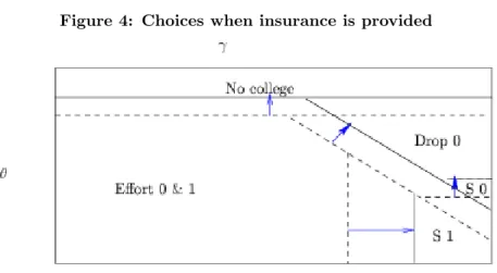
Figure 4: Choices when insurance is provided
Figure 4 indicates the effects of optimal insurance. Insurance increases the value of going to college and, thus, shifts up the the γ0 and γ1 loci. Thus, insurance increases the fraction of students putting in effort
in both periods. If optimal insurance requires f0 > 0, then it shifts down the θ0 locus – of the students
who choose not to put in effort in college in period 0, a bigger fraction choose to continue on in college and shirk. Both effects work to lower dropout rates in period 0. Dropout rates also decline in period 1 because
γ1shifts up and all those who do not put in effort either continue to drop out or shirk – the latter happens
if optimal f1 ≥ f¯1. The effect of optimal insurance on the non-completion rate is ambiguous because it
encourages some students who were dropping out to put in effort (this is the positive effect) and others who were dropping out to shirk (the negative effect). Of course, optimal insurance raises the enrollment rate. It is an open question whether optimal insurance should tolerate some amount of shirking. Providing insurance beyond the “no-shirking” level will encourage more enrollment and more effort in college but it will also cause some students to shirk and thereby increase the cost of providing the insurance.
Note that the insurance friction here is entirely about adverse selection. Optimal insurance never encourages anyone who was putting in effort in college to stop putting in effort. Indeed, it encourages people who were not putting in effort to put in effort. The friction is simply that some students who were choosing to drop out may choose to continue on in college without putting in effort (there is no change in their college effort decision). Thus, insurance attracts students whose failure probability is 1. This is an extreme form of adverse selection.
Some additional comments are worth making. First, we are implicitly assuming that once a student fails college, he or she never attempts college again. If we were to relax this assumption, the insurance arrangement would need to specify that once a student avails herself of insurance, she cannot re-enroll in college without re-paying the indemnity with interest.
Second, we are abstracting from the adverse effects on the private returns to college education that may stem from policy-induced increases in college completion rates.10 On the other hand, we are also abstracting
from the myriad social benefits of a more educated populace.
Finally, the following caveat should be kept in mind regarding the optimality of the insurance arrangement. Because higher education is subsidized by federal and state governments, changes in enrollment and com-pletion rates induced by insurance will change the level of subsidy being received by the higher education sector. The welfare costs of this additional subsidy are being ignored here.
5
Mapping the Model to Data
The first issue that must be dealt with is that students vary in their probability of successπ. Furthermore, the insurance arrangements discussed in the previous section assume that each student’sπ is observable to student loan administrators. So the first task is to pool students with respect to some observable index of the probability of success in college. We use SAT scores for this purpose. In particular, we classify students in 5 groups. Table 2 gives the distribution in 1999 of students who took the SAT.
Table 2: Distribution of SAT scores
SAT scores
0
−
699
700
−
900
901
−
1100
1101
−
1250
1251
−
1600
Fraction 0.079 0.224 0.342 0.205 0.15
In what follows, we will consider only the four top groups. We will denote these groups by the index
i∈ {1,2,3,4,}.
There are 4 parameters and 4 distributions in the model. Among the parameters are 2 preference parameters
σand β and 2 college parametersxandπ. Among the distributions are distributions for the (unobserved) heterogeneityF(θ) andG(γ) and the distributions of earnings of non-college and college workers H(y) and
M(y). We assume that all students have the same preference parameters and draw from the same distribution of the “outside option”F(θ) but we allow the parametersx and π and the distributions G(γ), H(y) and
M(y) to depend oni. Naturally, we expect π(i) to increase withi. We also expect the distributionG(γ) to depend on i because the utility cost of exerting effort in college is, plausibly, more likely to be lower for a student with a higher SAT score. We also expectxto depend onibecause students with higher SAT scores tend to go to more selective colleges and these colleges tend to have higher tuition.11 This tendency forx
10Card and Lemieux (2001) as well as Bound, Lovenheim, and Turner (2009) find evidence of congestion effects in higher
education: an increase in the number of people seeking higher education tends to be associated with a decline in educational attainment.
11We do not explicitly analyze the matching of students of varying ability to colleges of varying selectivity, but our
to increase with i is partly offset by the tendency of more selective colleges to provide more financial aid. Finally, if scholastic ability is correlated with ability more broadly (as seems plausible), we also expectH(y) andM(y) to depend oni. In particular, we would expect students with higher SAT scores to be more likely to draw a highery.
5.1 Preference Parameters, Earnings Distributions and College Costs
We assume that the utility function is given by
U(c) = (c+)1−σ/(1−σ) ifc >0 1−σ/(1−σ) ifc≤0
where is a small positive number. Thus the utility function is defined over the real line but is effectively CRRA with coefficient of relative risk aversion ofσforc >>0. We setσ= 2 andβ= 0.97, both conventional values in quantitative macroeconomics.
In the theory, y is the person’s lifetime earnings. We calibrate the lifetime earnings distributions using earnings data from the CPS for 1969-2002 for synthetic cohorts. There are 5000 observations in each year’s sample, on average. We distinguish between two education groups: those with at least 12 years but less than 16 years of completed schooling and those with at least 16 years of completed schooling. The former corresponds to the non-college group and the latter to the college group. For each education group, we calculate the mean real earnings of heads of households who are 25 years old in 1969, 26 years old in 1970, . . . , 58 years old in 2002.12 The mean present value of life-cycle earnings for each group is simply the sum of
the mean earnings at each age.13 For the non-college group mean life-time earnings is $1.07 million and for
the college group it is $1.69 million. These estimates imply a college premium of 58 percent. Micro-studies find that the increase in lifetime earnings from each additional year in college is between between 8% and 13% (see Willis (1986) and Card (2001)). Since the average college graduate has more than 4 years of college education (some students do post-graduate schooling), our calibration of the college premium is roughly consistent with the high end of this range of estimates.14
To estimate the variation of lifetime earnings around these mean values, we assume that the life-time earnings
on the importance of individual characteristics coupled with college characteristics for college attendance and completion, see Bound, Lovenheim, and Turner (2009), Hastings, Kane, and Staiger (2006), Hoxby (2004) and Light and Strayer (2000).
12To increase the number of observations in each age group, we consider five-year bins. That is, by age 25 in 1969 we mean
heads of household who are between 23 and 27 years old (both inclusive) in that year. Real values are calculated using the CPI for 1999
13Ignoring discounting overestimates life-time earnings and ignoring earnings beyond age 58 underestimates it. 14Restuccia and Urrutia (2004) use a 10% rate of return, which corresponds to a lifetime college premium of about 1.5.
of an individual in education groupkare given byz(µk25+µk26+· · ·+µk58), wherezis a random variable with
mean 1 and varianceσ2
z(k) andµknis the mean earnings in education groupkat agen. Then,σz(k) is simply
the (common) coefficient of variation of earnings at any agenin education group k. We setσz(k) equal to
the mean coefficient of variation in earnings across all ages in education groupk. This construction implies that the standard deviation ofy is $ 0.8 million for the college group and $ 0.5 million for the non-college group.
The above calibration of the mean and standard deviation of lifetime earnings for the two education groups is for each group as a whole. Within each group, we permit the distribution of lifetime earnings of individuals to vary systematically with scholastic ability (see Cunha and Heckman (2009), Hendricks and Schoellman (2009)). We use the data set High School and Beyond (HS&B) to group students by the four ability groups
i ∈ {1,2,3,4} and compute the mean earnings for each group of those students who are five years out from the year they acquired their highest degree and are employed full-time. We use these mean earnings to compute the mean earnings of each ability group relative to the overall mean earnings of the education group in question and then apply these relative mean earnings factors to the mean earnings in the CPS data for the corresponding education group. This yields (µC
i (y),i = 1,2,3,4) = (1.66,1.74,1.84,1.91) and
(µN C
i ,i = 1,2,3,4) = (1.05,1.11,1.17,1.21).15 We assume that the standard deviation of earnings for each
ability group is the same as for the group as a whole. Finally, in order to compute the relevant expected utility values, we assume that all earnings distributions are Normal.
The cost for college was $20,706 per year for private universities and $8,275 per year for public universities in 1999. Among the students who borrowed for their education, 67% went to public and 33% to private universities. The enrollment-weighted total college costs are $49,508 in 1999 dollars (College Board (2001)). We consider heterogeneous costs of college. Using the same enrollment-weighted procedure, we estimate college costs across ability groups using data from the Princeton Review on college rankings in terms of average SAT scores of accepted students and data from USA Today on college costs (tuition and room and board). We estimate college costs for the 4 groups of ability levels to be: $35,200, $37,000, $56,400, and $73,400 (in 1999 dollars). Thus, we find that high ability students enroll in more expensive colleges (more selective colleges tend to be more expensive). We set college costs (in millions) (2xi,i=1,2,3,4) =
(0.0352,0.0370,0.0564,0.0734).
15We use the HS&B because the B&B data set (which reports earnings for more years) covers only college graduates while
the BPS data set covers both high school and college graduates but reports earnings only upon graduation. Since earnings differentials due to ability are likely to manifest themselves gradually over time, using earnings information from some years out is preferable. We normalize the units in which earnings are measured in the model so that 1 unit means $1 million.
5.2 Completion Probabilities and Distributions of Disutility from Effort
To calibrate πi, we use the Beginning Postsecondary Student Longitudinal Survey (BPS 1995/96), which collects data on intensity of college attendance and completion status of post-secondary education programs for students who enrolled in 1995.
We consider only students who enroll without delay in either 2- or 4-year colleges following high school graduation. Because we do not have part-time enrollment in the model, we consider students who enroll exclusively full-time in their first academic year and enroll full-time in their first and last months of enrollment in future academic years.16 The survey records the fraction of students (for each ability group) who, in 2001, report having earned a bachelor’s degree. This is thedegree completion rateand for our universe of students comes out to be (ci,i=1,2,3,4) = (0.601,0.72,0.825,0.871).17 These rates do not identify πi because the
universe includes students who do not put effort in college; for instance, it includes students who drop out shortly after enrolling and therefore never earn a degree. To identify πi, we first locate students who, in
2001, report not having earned a bachelor’s degree and who report having last enrolled in academic years 1995-96 or 1996-97. This group is our empirical analog of students who drop out or fail in period 0 or drop out at the start of period 1. We refer to this group asleaversand their fraction (in our universe of students) comes out to be (li i=1,2,3,4) = (0.088,0.056,0.025,0.013).18 The complement set is our empirical analog
of students who are in good standing at the start of period 1 and who put in effort in college. Therefore, we obtain (πi i=1,2,3,4) = ((0.601/(1−0.088),0.72/(1−0.056),0.825/(1−0.025),0.871/(1−0.013)) = (0.659,0.7627,0.8462,0.8825). Observe thatπis increasing in SAT scores, which justifies our initial thought that SAT scores are an observable proxy forπ.
The calibration of the distributionsF(θ) andGi(γ) is achieved via moment matching. The moments we target are enrollment and leaving rates for the four ability groups. We use the National Education Longitudinal Study (NELS:88) to collect information on the college enrollment choices of students who were high school seniors in 1992. We consider a student to be enrolled in college if he or she enrolled without any delay after high school and was enrolled in either a 2-year or 4-year colleges in October 1992. The enrollment rates by our four ability groups comes out to be (ei i=1,2,3,4) = (0.795,0.894,0.943,0.957).
We assume thatF is distributed normal with meanµθand standard deviationσθand theGi(γ) is distributed
16Since students can enroll full-time but drop out shortly thereafter, “exclusively full-time enrollment in the first academic
year” simply means that the student is enrolled full-time for the months he or she is actually enrolled. For later academic years, we weaken the full-time requirement to apply to only the first and last months of enrollment. This allows students to go part-time for short stretches of time.
17We did not want the college performance of students with very low and very high SAT scores to overly affect the performance
of their respective groups (the 700−900 group and the 1250−1600 group). We employed a 5% Winsorization with respect to SAT scores to reduce the sensitivity of group performance to outliers.
exponential with mean µγi. These distributional assumptions imply that there are 6 parameters to be
constrained by 8 moments. The problem reduces to finding the vector of parametersα= (µθ, σθ, µγi=1,2,3,4)
that solves min α 4 X i=1 wi((ei−ei(α))2+vi(li−li(α))2 ! ,
where ei(α) andli(α) are the corresponding model rates and wi and vi are the weights assigned to these
rates.
Table 3: Enrollment and leaving rates: model and data
SAT scores
700
−
900
901
−
1100
1101
−
1250
≥
1251
Enrollment rates : Data0
.
795
0
.
894
0
.
943
0
.
957
Enrollment rates : Model0
.
77
0
.
908
0
.
949
0
.
961
Leaving rates: Data0
.
088
0
.
056
0
.
025
0
.
013
Leaving rates: Model0
.
088
0
.
043
0
.
025
0
.
013
Table 3 gives the outcome of this moment matching exercise. As is evident, the match between data and model moments is quite good. We find the distributionsF(θ)∼(0.39,0.21) andG1(γ)∼(0.066),G2(γ)∼(0.065),
G3(γ)∼(0.057), andG4(γ)∼(0.046). Note that means of the γ distributions decline with ability. This is
consistent with our interpretation ofγ as the utility cost associated with school work. High-ability students seem to bear fewer costs (i.e., find the work more enjoyable) than low-ability students.
6
Insurance Against Failure Risk
In this section we report the results regarding insurance for each of the 4 ability groups. We follow the structure of the analysis in Section 4. For each ability group (i.e., for eachπ) we consider the best possible insurance when (i) effort is observable, (ii) effort is not observable and the insurance must respect the no-shirking constraint, and (iii) effort is not observable and shirking is tolerated.
6.1 Full Insurance
First, we consider the case where effort is observable. The model delivers that the level of insurance that equates marginal utilities across states,fi∗, is 0.076,0.104,0.143,0.172 fori= 1, ...4. These levels are higher than the cost of college, 2xi, for all ability levelsi (they represent 216.5%, 280.8%, 253.6%, and 234.5% of college costs by ability groups). Thus our calibrated economy satisfies Assumption 5. So, when effort is observable, it is optimal to insure students of all ability groups up to the full cost of college.
6.2 No-shirking Insurance
Recall from Proposition 4.2 that an optimal no-shirking insurance must offerf0= 0 in period 0 and up to ¯fi1
in period 1, where ¯fi1 satisfies
´
U(y−5xi/4)dHi(y) =β
´
(y−2xi+ ¯fi1)dHi(y) (hereHi is the non-college
distribution of earnings of ability group i). An important observation is that when this level of insurance is provided, there is a positive mass of students who are indifferent between shirking and dropping out in each ability group. Our assumption is that if a student is indifferent between shirking and dropping out, she shirks. Given that, we consider giving an indemnity of 1% less than the level that makes shirking just as good as dropping out. Thus, we offer ¯fi¯1 = 0.99 ¯fi1 in case of failure and the premium that is paid in case
of success is ¯¯si1= (1−πi) ¯fi¯1/πi.
Table 4 presents the indemnity offered, ¯f¯i1, by ability groups, as well as the premium paid in case of success,
¯ ¯
si1, as percentages of the cost of college. The indemnity offered increases in ability, with the top ability
group receiving more than two times more indemnity than the bottom ability group. However, given that the college cost increases in the ability level, each ability group is forgiven a roughly constant fraction of their college cost in the case where failure occurs. The bottom/highest ability group is forgiven 23.3%/24.6% of their college cost. The insurance, however, is more expensive for the low-ability groups relative to the high-ability groups: the premium is 12.1% of the college cost for the bottom ability group and only 3.3% of the college cost for the top ability group.
Table 5 displays how enrollment, leaving and completion rates change with the insurance. Since insurance increases the value of putting in effort in college, givenθthere is less chance a student will want to drop out of college. Thus, there is a tendency for leaving rates to go down and completion rates to go up. On the other hand, there is a selection effect working in the opposite direction. Because insurance increases the value of putting in effort in college, it also increases enrollment. The new enrollees are students with low values ofθ. Since theγ0(x, θ, π) locus is increasing inθ, the new enrollees are more likely to drop out in period 0. For the
first three ability groups, the first effect dominates and insurance causes leaving rates to fall and completion rates to rise. For the top ability group, the second effect is decisive. For this group, insurance encourages everyone to enroll and there is a sufficiently large increase in the share of “low θ” students so that leaving rates rise and completion rates fall.
Table 5 also displays the welfare gain from insurance, namely, the percentage increase in welfare with insur-ance relative to the no-insurinsur-ance (baseline) model. As we might expect, the insurinsur-ance is most valuable to students with a high probability of failure and, indeed, the welfare gains decline with rising ability.19
19These gains are in the nature of social welfare gains where the social welfare function treats students with differentθvalues
Table 4: No-shirking insurance SAT scores
700
−
900
901
−
1100
1101
−
1250
≥
1251
Indemnityf1 0.0082 0.0084 0.0134 0.018 Percentage of 2x 23.34 22.74 23.7 24.55 Premiums1 0.0043 0.0026 0.0024 0.0024 Percentage of 2x 12.08 7.61 4.31 3.27Table 5: Enrollment, leaving and completion rates: no-shirking insurance SAT scores
700
−
900
901
−
1100
1101
−
1250
≥
1251
Enrollment rates with insurance0
.
848
0
.
924
0
.
965
1
Enrollment rates : data0
.
795
0
.
894
0
.
943
0
.
957
Leaving rates with insurance0
.
032
0
.
030
0
.
020
0
.
015
Leaving rates: data0
.
088
0
.
056
0
.
025
0
.
013
Completion rates with insurance0
.
638
0
.
740
0
.
829
0
.
870
Completion rates: data0
.
601
0
.
720
0
.
825
0
.
871
Welfare gains in percentage2
.
83
2
.
38
2
.
06
1
.
86
6.3 Optimal Insurance
We consider the general insurance case wherefi ∈[0, x]×[0,2xi]. For comparison purposes, we first show the results if insurance is offered only in period 1.
The first task is to determine the set of feasible insurance schemes for each ability group. When insurance is offered only in period 1, an insurance arrangement f = (0, f1), f1 ∈ [0,2xi], is feasible if there exists a τi∗1(f) such that equation (2) is satisfied for ability group i. Obviously, any fi1 < f¯i1 is feasible because
there is no shirking and τ1 = 0 will trivially satisfy the feasibility condition. To determine feasibility for
f1≥fi¯, we divide [ ¯fi1,2xi] into a fine grid and for each grid point attempt to find aτthat satisfies (2). Our
procedure is to iterate onτ1. For iterationk, we setτ1k to the value that satisfies (2) given the decision rules
corresponding toτ1 from iteration k−1 (i.e.,τ1k−1). We start the iterations with τ10 = 0. If this iterative
process converges we classify that particular grid point as feasible. If the process diverges, we classify it as infeasible.
We find that the feasible indemnity levelsf1 ∈[ ¯f1,2x] differ across ability groups. These sets turn out to
be ∅, [23.8,29.8], [24,34.8], [25.9,50.5] (numbers are given in % of the college cost, 2xi) fori= 1,2,3,4. No
insurance including and beyond ¯f1 1is feasible for the lowest ability group. For the other three ability groups,
insurance levels beyond ¯fi1are feasible. More f are feasible for higher ability levels.
These sets highlight the adverse selection problem. In the bottom ability group the probability of successπ