An analysis of foreclosure rate differentials in soft markets

w o r k i n g

p

a

p

e

r

F E D E R A L R E S E R V E B A N K O F C L E V E L A N D

08

11

An Analysis of Foreclosure Rate

Differentials in Soft Markets

Working papers

of the Federal Reserve Bank of Cleveland are preliminary materials circulated to

stimulate discussion and critical comment on research in progress. They may not have been subject to the

formal editorial review accorded offi cial Federal Reserve Bank of Cleveland publications. The views stated

herein are those of the authors and are not necessarily those of the Federal Reserve Bank of Cleveland or of

the Board of Governors of the Federal Reserve System.

Working Paper 08-11

November 2008

An Analysis of Foreclosure Rate Differentials in Soft Markets

by Francisca Richter

A quantile regression model is used to identify the main neighborhood

charac-teristics associated with high foreclosure rates in weak market neighborhoods,

specifi cally for two counties in Ohio and one in Pennsylvania. A decomposition

technique by Machado and Mata (2005) allows separating foreclosure fi ling rate

differentials across counties into two components: the fi rst due to differences in

the levels of neighborhood characteristics and the second due to differences in

the model parameters. At higher than median rates, foreclosure rate differentials

between counties in Ohio are mainly explained by the levels of these

character-istics. However, foreclosure rate differences between counties across states are

mainly explained by the parameter component, suggesting that state level effects

might have contributed to shape foreclosure rate outcomes.

Key words: foreclosure, quantile regression, decomposition analysis.

JEL code: G21, R23

I. Introduction

Recent studies have contributed to identifying traits and commonalities of high foreclosure rate neighborhoods (Grover, Smith and Todd, 2008). Currently, there seems to be a

consensus in that the mortgage crisis unfolded differently in regions with strong as opposed to weak or soft real estate markets. Differences in weak and strong markets lie in the

economic and housing market conditions under which the crisis took place. The consistent home price appreciation from 2000 to 2005 at the national (aggregate) level was driven by steeper appreciation in these strong markets, while in soft ones real home prices remained virtually unchanged. As credit was expanded, weak markets with little or negative population growth experienced a higher share of subprime originations in areas of previously high denial rates (Mian and Sufi, 2008). Mayer and Pence (2008) also find that lending activity in depressed housing markets is more likely to be subprime. At the same time, these markets’ high rates of foreclosure were coupled with previous high rates of vacancy and abandonment contributing to the worsening of spillover effects in

neighborhoods (Community Research Partners, 2008). This is the case in Ohio, and particularly Cleveland, reported among the top cities in regards to foreclosure rates and vacancy.

However, even among the weaker housing markets, foreclosure rates varied considerably in 2007. For instance, despite similar conditions in the housing market and demographic variables for individuals and neighborhoods in Cuyahoga (Ohio) and Allegheny (Pennsylvania), the distributions of census tract foreclosure rates in these counties were quite different, with Cuyahoga displaying the largest variation. Thus, it would seem that differences in foreclosure rates across these counties can only partly be explained by demographic and neighborhood differences.

Differences in the regulatory environment across states may also contribute to differences in the quality of loans originated, and ultimately, the rates of foreclosure. An effective

regulatory environment that reduces information asymmetries and promotes a better functioning of the markets ultimately enhances net social surplus. In the home mortgage market, in particular, lower foreclosure rates may be expected with better regulations. At the same time, characteristics such as low income level, high rates of vacancy in the neighborhood, and low credit scores are all expected to positively correlate with higher neighborhood foreclosure rates. However, all else being equal, an effective regulatory environment should be conducive to weakening the negative impact of low income

individual and neighborhood demographics on foreclosure rates. It is under this framework that the impact of regulations is explored here, in its interaction with demographic and neighborhood characteristics associated with high foreclosure rates. Unlike this approach, previous studies of the effect of regulations on subprime loan originations or foreclosures use indices of state regulatory strength or enforcement and measure their impact after accounting for demographic characteristics (Ho and Pennington-Cross, 2005).

This paper has two main objectives: (a) identify the main neighborhood characteristics associated with high foreclosure rates in weak markets neighborhoods, and (b) identify any possible differences in the impact of these variables (as measured by model parameters) that might explain across versus within state foreclosure rate differences. Since regulatory effects are likely to be among the most important state-level effects, findings from this exercise would suggest the degree to which differences in regulations contributed to the differences in foreclosure rates between Allegheny and two Ohio counties, Cuyahoga and Franklin. The methodology to accomplish these objectives can be broken down into three components listed here and detailed in the remaining of this section: (1) Estimate quantile regression

models of foreclosure rates, since high foreclosure rates (a tail phenomenon) are of interest. (2) Use the quantile regression models to estimate counterfactual distributions of foreclosure rates in county A when demographic characteristics are as in county B. (3) Use the

counterfactuals to decompose foreclosure rate differentials across counties into two

components: one due to differences in the levels of neighborhood characteristics (covariates) and the second due to differences in the model coefficients.

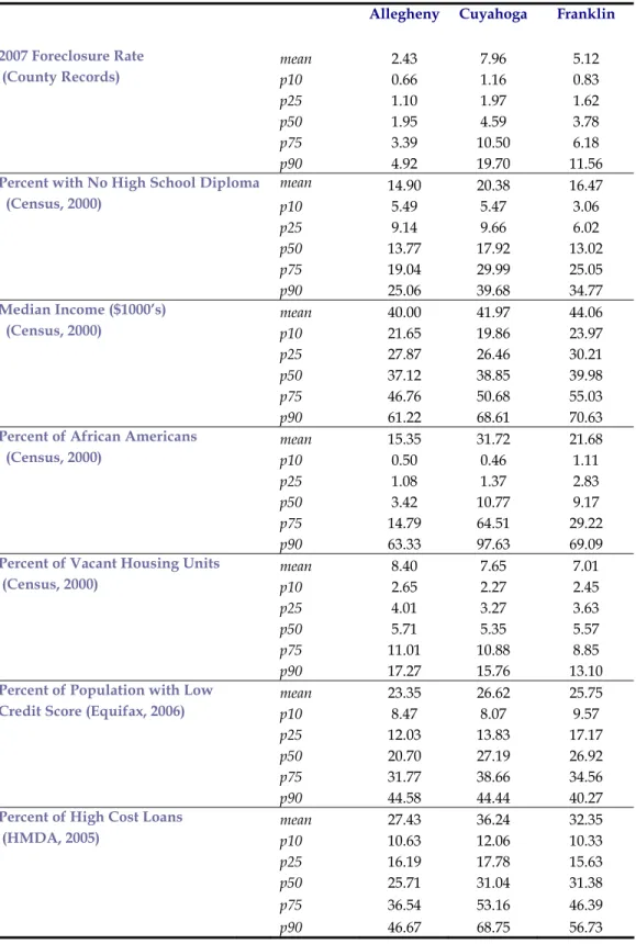
The analysis is performed using foreclosure filing rates at the census tract level for three counties: Cuyahoga and Franklin in Ohio, and Allegheny in Pennsylvania. The geographic proximity and demographic similarity of these counties (table 1) provides a good ground for comparing their less similar foreclosure rate distributions. Models for within and across state foreclosure rate differences allow capturing state level effects on foreclosure rate distributions. And while regulatory variables are not explicitly included in the model, they are likely to be among the most important state-level effects.

(1) Quantile regression models of foreclosure rates

Most research on determinants of high foreclosure rates at the regional level use regression analysis to estimate the relationship of neighborhood and loan characteristics and/or regulation with the mean foreclosure rate or a function of it. This approach is appropriate when the focus is on neighborhoods with average foreclosure rates, or when it is safe to assume that covariates equally determine foreclosure rates in high as in low foreclosure-density neighborhoods. However, foreclosure rates exhibit wide variability across

neighborhoods and part of the focus of this study is to understand what is different in high versus low foreclosure density areas. The fact that the impact of the covariates may vary with the concentration of foreclosures supports the use of quantile regression in this study.

Quantile regression allows estimating the relationship between covariates and foreclosure rates at any specified quantile of the distribution.

(2) Counterfactual distributions

The analysis goes further to explore how much of the foreclosure rate differential in these counties can be explained by borrower and neighborhood characteristics as opposed to other factors that may have contributed to the outcomes. In other words, how would Allegheny borrowers and neighborhoods have performed under Cuyahoga (Franklin) environment and vice versa? The environment here includes but is not restricted to laws and regulation regarding the mortgage market. Here again, the analysis is performed over the whole distribution of foreclosure rates rather than the mean only.

(3) Decomposition of foreclosure rate differentials

The methodology used is based on the Machado-Mata (2005) method (MM) to explain wage differentials across time or geography. The MM method allows decomposing the differences in the log wage distributions (across time or geography) in two parts: the first, explained by differences in the levels of relevant characteristics (such as education), and the second, explained by differences in the returns to those characteristics. Returns, in this case, measure the relevance or value attached to characteristics such as education by each geography or time period, as measured by wages.

Similarly, one is able to decompose the differences in foreclosure filing rates across two counties into two parts. One component of the rate differential is due to differences in the level of neighborhood characteristics or covariates. An example of a level measure is the percent of borrowers with low credit score in the neighborhood. The second component, however, has to do with the way the county values (penalizes) these characteristics, as

measured by lower (higher) foreclosure rates. Factors that influence this second component include laws, regulations and state and city procedures regarding consumer protection. This approach contributes to current efforts to assess the impact of laws and regulation by means of indices of regulatory strength and enforcement as explanatory variables for subprime originations and foreclosure rates. For instance, a study by Bostic et al. (2008) construct state and local indices of anti-predatory lending laws to be used as explanatory variables of subprime originations. These indices include mini-HOEPA laws and older laws. Index values for Ohio are equal or larger than for Pennsylvania. In order to eliminate the effect of missing variables that might affect subprime originations across states, a border pair geographic sampling method is used. Mortgage broker laws and regulation have also been studied (Kleiner and Todd, 2007) based on state indicators. Indicators measure restrictiveness based on licensing and registration policies (Pahl, C. 2007) of mortgage brokers. The analysis is performed with state level regulatory-related indices. Here again, Ohio’s values are larger than Pennsylvania’s.Indices cannot avoid introducing subjectivity to the analysis to a greater or lesser extent. They represent a weighted or simple average of numerical values attached to certain characteristics of laws according to their level of relevance as determined by an expert. Indices are more likely to measure quantity over quality of regulations. While this study’s approach does not rely on the use of such indices, it does not isolate the effect of the legal and regulatory environment either. At best, it measures the impact of a broader set of norms and behaviors (or lack thereof) –in part governed by the legal and regulatory environment- on the distinct patterns in which foreclosures have taken place throughout the counties. Rather than making assumptions about the ways in which individual regulations combine to affect outcomes, this approach assumes that, all else being equal, a more effective regulatory environment will translate

into a decreased correlation between low income neighborhood characteristics and negative outcomes. Therefore, differences in regulations across states that impact foreclosure rates may be captured through differences in the strength of correlation of these variables with foreclosure rates (coefficient effect), while at the same time acknowledging the effect of differences in the level of neighborhood variables (covariate effect).

II. Data and Methodology

The least squares regression model has been referred to as a pure location shift model because it assumes that covariates x only affect the location, but neither scale nor shape of the conditional distribution of y (Koenker and Hallock, 2001). In that sense, a set of quantile regression models is less restrictive and better suited to characterize the conditional

distribution of y throughout its entire range. A particular feature of quantile regression that appeals to the analysis of foreclosure rate data is that it is robust to extremes in the

dependent variable (Koenker and Hallock, 2001). Thus, it provides a more accurate

description of the tails, which here represent high foreclosure rate regions, a main focus of this work.

For each county, the following conditional quantile regression model is estimated:

5 1

0 1 0 1

y / p ,p k k ,p k

F−_x( p x) =Q ( y x) =

β

+

∑

₌

β

x , p∈( , ) (2.1)

where

Q ( y

_p

x

)

is the pth _{conditional quantile of the (log odds) unduplicated foreclosure} filing rate distribution in census tracts across the county,

y

=

ln ( z (

1

−

z ) )

. F_{y /x}( y x) is the cumulative distribution function of y conditional on x. The explanatory variables or covariates x are as follows: percent population with no high school diploma, median income, percent of African American population, percent of vacant housing, percent of

population with low credit score, and percent of high cost loans. The first four variables are from the 2000 census. The credit variable is based on a sample of 2006 Equifax scores, where low credit is defined as being less than 639 points. The percent of high cost loans is from the Home Mortgage Disclosure Act data (HMDA 2005) and includes all loans with annual percentage rate at least 3 percentage points greater than the yield of a treasury security of comparable maturity. All variables except the low credit percent are in logs to allow for a linear specification of (2.1). The explanatory variables describe borrower and neighborhood, as well as loan characteristics. It is reasonable to hypothesize that loans made to individuals with lower levels of education, income and credit score are at a higher risk of foreclosure. At the neighborhood level, this translates into higher foreclosure rates. But even when accounting for income, race of the borrower (or race composition in neighborhoods) has been shown to be a significant regressor in explaining foreclosure risk and rates (Coulton et al., 2008; Mayer and Pence, 2008). Higher vacancy and abandonment rates signal higher housing market distress and is hypothesized to correlate with higher foreclosure rates. Similarly, higher levels of high cost loans in a neighborhood are may lead to higher chances of predatory lending, and therefore, higher foreclosure levels. Other variables tested but not included to avoid multicolinearity were percent of unemployment, population below poverty, and percent of loans issued by subprime lenders (HMDA definition).

A set of parameters

β

_0,p

,

_K

β

_5,pfor any p value between 0 and 1 estimates the effect of the independent variables at the pth _{quantile of the (log odds) foreclosure rate distribution. For a} sample of size n, the parameter vector β_p =

(

β

_0,p,_K

β

_5,p

)

′is calculated to minimize the following weighted sum of errors:

1

1

where

n _{i i p} i ,p i i p i ,p i i i p

p

if y

w ( y

),

w

p

if y

=

⎧

_≥

′

⎪

′

−

_{= ⎨}

′

−

<

⎪⎩

∑

x

β

x

β

x

β

(2.2)

Here, yi is the sample (log odds ratio) foreclosure rate for census tract i and xi is the vector of explanatory variables for census tract i. When p is 0.5, (2.1) is a median regression and parameters estimated by minimizing (2.2) are known as MAD (mean absolute deviation) estimators. Quantile regression, thus, allows characterizing the effects of the covariates at different points of the conditional distribution of foreclosure rates for census tracts in a given county. Parameter estimates for each covariate can be plotted against their corresponding quantiles with empirical confidence bands displaying their statistical significance and the strength of their correlation with the dependent variable throughout its entire distribution. The unconditional or marginal distribution of (log odds ratio) foreclosure rates in county A, consistent with model (2.1) can be estimated according to the MM method. The probability integral transformation theorem states that if y is a continuous random variable with cumulative distribution function F(y), then

p

=

F( y )

Uniform( , )

0 1

. A corollary of this

theorem implies that 1

p

Q

=

F ( p)

−

F( y )

, provided the inverse CDF of y exists. Thus, if p is randomly chosen from a

Uniform( , )

0 1

, and assuming model (2.1) holds, it follows that

p i p

Q

=

x

′

β

is a random value from the conditional distribution of y given xi. Then, an

estimated sample from the marginal distribution of log odds foreclosure rates is obtained by bootstrapping from the sample x’s and computing

{

}

1

( i ) p( i ) i=....m ′

x β

.

This is equivalent to integrating x out of the conditional sample. The process is as follows:

(1) generate a random sample of m values in (0, 1) and use sample

1

,

n

′

⎡

⎤

= ⎣

⎦

X

x

_K

x

and

y

in A to estimate the corresponding sets of quantile parameters

p( 1 ) p( 2 ) p( m )

(

,

,

)

=

β

β

β

_K

β

(2) generate a bootstrap sample of covariates from

{ }

1 i _{i=, ,n} x K (in A) of size m, 1 ( )

,

,

( m )

′

⎡

⎤

= ⎣

⎦

m

X

x

_K

x

(3) compute

{

}

1 ( i ) p( i ) i=, ,m

′

x

β

K .

This gives a sample of size m from the unconditional log odds ratio of foreclosure rates distribution in A as predicted by the modelˆy( z ;_A X_A), from which the distribution of foreclosure rates

ˆf( z ;

_A

X

_A

)

can be characterized.

A similar procedure is used to obtain samples from counterfactual distributions, such as the foreclosure rate distribution that would have prevailed given covariates as in county B and parameters as in county A:

(1) generate a random sample of m values in (0, 1) and use

X

= ⎣

⎡

x

₁

,

_K

x

_n

⎤

_⎦

′

and

y

in A to estimate the corresponding sets of quantile parameters

p( 1 ) p( 2 ) p( m )

(

,

,

)

=

β

β

β

_K

β

(2) generate a bootstrap sample of covariates from

{ }

1 i _{i=, ,n} x K (in B) of size m, 1 ( )

,

,

( m )

′

⎡

⎤

= ⎣

⎦

m

X

x

_K

x

(3) compute

{

}

1 ( i ) p( i ) i=, ,m

′

x

β

K .

This constitutes a sample of size m from the (counterfactual) unconditional log odds ratio of foreclosure rates distribution that would have prevailed in A if covariates would have been distributed as in B. This counterfactual distribution is estimated by the modelˆy( z ;_A X_B), from which the distribution of foreclosure rates

ˆf( z ;

_A

X

_B

)

can be characterized. In both cases, the sample size m is 4000.

This analysis is of interest because the quantile parameter variation across counties responds to variations in the way each county values or penalizes borrower and loan characteristics. Take for instance Cuyahoga covariates, i.e. the percent of high cost loans, percent of high school graduated, etc. How would have foreclosure rates been distributed in Allegheny and Franklin if covariates in these counties had been as in Cuyahoga? And how much of the foreclosure rate difference is explained by differences in the covariates as opposed to differences in the parameters?

To answer the latter question, assume random samples corresponding to the following marginal distributions in Cuyahoga (C) and Allegheny (A) have been computed using the MM method: ˆy( z ;_C X_C), y( z ;ˆ _A X_A), y( z ;ˆ _C X_A), y( z ;ˆ _A X_C).

If the function

α

is a summary statistic_ say the median of the sample_ then the actual (log odds ratio) foreclosure rate difference is the estimated difference plus a residual:

C A ˆ C C ˆ A A

( y( z )) ( y( z )) ( y( z ; )) ( y( z ; ))

α

−

α

=

α

X −

α

X +

ε

(2.3)

Adding and subtracting ˆy( z ;_C X_A)to the right hand side of (2.3) and grouping terms results in: C A C A A A C C C A ( y( z )) ( y( z )) ˆ ˆ ˆ ˆ ( y( z ; )) ( y( z ; )) ( y( z ; )) ( y( z ; )) α α α α α α ε − = − + − +

⎡

⎤ ⎡

⎤

= ⎣

X X

⎦ ⎣

X X

⎦

(2.4)

The first term in brackets measures the difference in the median value due to county

parameter differences estimated by the model and given covariates as in A. The second term is the difference in the mean of rates due to county covariate level differences estimated by the model and given parameters as in C. A similar decomposition can be obtained by adding and subtracting the termˆy( z ;_A X_C), only in this case, median differences due to county parameter differences are estimated given covariates as in C. Likewise, median differences due to county covariate level differences are estimated given parameters as in C. Although the decomposition technique has been described for the median,

α

represents any summary statistic, in particular quantiles. Since the log odds ratio of foreclosure rates

1

y =ln( f / ( −f )) is the dependent variable in the estimated model (2.1), the decomposition is done on this variable. The decomposition is applied to paired differentials for the three counties (Cuyahoga – Allegheny, Cuyahoga – Franklin, Allegheny – Franklin). Summary statistics computed are the 10th_{, 25}th_{, 50}th_{, 75}th_{, and 90}th _quantiles.

III. Results

Figure 1 shows the distribution of 2007 foreclosure rates for the Allegheny, Cuyahoga, and Franklin counties. Foreclosure rates are calculated as 2007 unduplicated foreclosure filings1 divided by the number of estimated mortgaged units in 2007. This latter estimate is an extrapolation of the 2006 American Community Survey estimate to 2007, assuming the 2006-2007 mortgage growth rate equals the rate in 2000-2006. Foreclosure rates are for census tracts in the county with 50 or more estimated mortgaged units in 2007. The distribution of

1

Filing data come from Allegheny County Prothonotary, Franklin County Common Pleas Court (provided by Community Research Partners), and the Cuyahoga County Common Pleas Court (provided by Cleveland State University).

census tract - foreclosure filling rates exhibits a larger variation in Franklin and Cuyahoga as compared to Allegheny. Differences in the distributions are even more apparent in census tracts with rates above the median filling rate. While Cuyahoga and Franklin distributions, both have longer right tails than Allegheny, this tail is heavier for Cuyahoga. Cuyahoga not only exhibits the highest mean foreclosure rate, but the largest variation as well. Table 1 shows that mean foreclosure rate differences across counties is heavily affected by differences at quantiles larger than the median. Variables that are similarly distributed across counties are median income, percent vacant housing, and percent of population with low credit scores. Larger variations across counties hold for the percent of high school graduates, African Americans, and high cost loans, particularly above their respective median values. Variations for these variables, however, are not nearly as large as the foreclosure rate variations displayed.

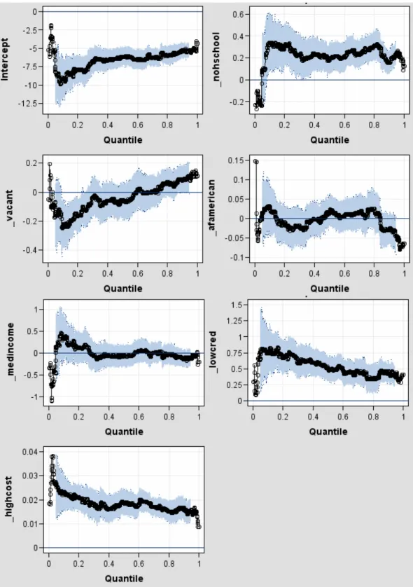
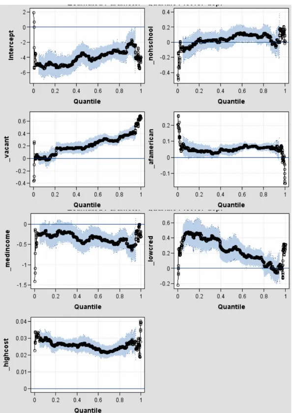
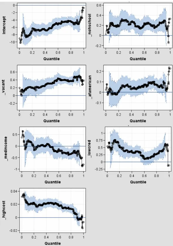
Figures 2, 3 and 4 show the estimated model parameters from equation (2.1) plotted against the foreclosure rate quantile range for Allegheny, Cuyahoga and Franklin counties

respectively. 90% confidence bands are displayed in blue. Covariates whose parameters are consistently significant through most of the quantile range and for all counties are the low credit score percent and high cost loans percent. The variable measuring percent of vacant properties in the tract is positive and significant through most of the range for Cuyahoga and Franklin. In Cuyahoga (and to a lesser extent in Franklin) the impact of vacancy

increases as foreclosure rates increase. It is interesting to note that while Allegheny reported slightly higher levels of vacancy in 2000 as compared to the other counties, this variable does not explain foreclosure rates in 2007. The fact that 2000 vacancy patterns in Cuyahoga and Franklin are consistent indicators of foreclosure rates in 2007 is suggestive of the persistence and relevance of vacancy and abandonment in these counties. On the other

hand, the impact of % high cost loans and % population with low credit score tends to decrease in general for the three counties as foreclosure rates increase, indicating a concave relationship between foreclosure rates and these neighborhood characteristics.

In Allegheny county parameters for median income and percent of African American population are insignificant, while the percent in the tract with no high school diploma is significant in explaining foreclosure rates. Franklin County exhibits a similar pattern, only that parameters for median income and African American percent are larger in magnitude and even significant around the 70th _{quantile of foreclosure rates. On the contrary, in} Cuyahoga, parameters for median income and percent African American are significant through most of the range, but the percent of high school graduates variable looses relevance. While median income is similar across counties, census tracts in Cuyahoga display a larger degree of geographic concentration of African American population (table 1), particularly in neighborhoods hardest hit by foreclosures.

Table 2 presents quantiles for the actual and estimated county distributions of foreclosure rates, as well as for the counterfactual distributions derived with the MM method applied to model (2.1). The estimated distribution of rates closely matches the actual distribution for the three counties. It is not surprising to see that if covariate levels in Franklin and

Allegheny had been as in Cuyahoga, foreclosure rates in the two counties would have been higher (see Cuyahoga characteristics in Franklin and Allegheny). Note however that higher rates are less noticeable for census tracts with foreclosure rates below the median. The increase in foreclosure rates is apparent in above median tracts for both counties, with the counterfactual Franklin rates moving closer to the actual Cuyahoga rates. It is worth noticing that while Franklin and Allegheny counties responded quite differently to

would have valued (penalized) Franklin and Allegheny covariates more homogeneously. This can be seen by comparing quantiles in table 2 for the counterfactual distributions corresponding to Franklin covariates in Cuyahoga and Allegheny covariates in Cuyahoga. Table 3 presents the decomposition analysis of the (log odds ratio) foreclosure rate

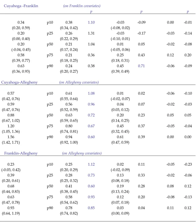
differences. The previous section outlined the decomposition method and referred to two equally valid ways to decompose rate differences into coefficient and covariate effects. Equation (2.4) is one of them and measures the covariate effect on Cuyahoga parameters. Results of this decomposition are presented in table 3. All terms in equation (2.4) are computed for the usual quantile levels. The first column corresponds to quantiles for the actual (log odds ratio) foreclosure rate difference between any two counties. The second column specifies the quantile. The third and fifth columns correspond to the estimated coefficient and covariate effect terms of the equation, and the seventh column calculates the residual at each of the quantiles. Columns four, six and eight express each of the three terms in (2.4) as a proportion of the actual rate difference (first column), giving a sense of the comparative relevance of both effects. Proportions are calculated independently of each other and are neither expected to add to 1 nor be restricted to the (0, 1) range. 90% bootstrap confidence intervals are provided for each quantile difference and corresponding effects. These are based on 3000 bootstrap samples.

The Cuyahoga - Franklin decomposition reveals that for census tracts with median

foreclosure rates and below, the covariate effect is much smaller than the parameter effect. For this range of tracts, the difference in levels of the explanatory variables account for little of the difference between foreclosure rates in the two counties. At the 25th _{quantile the} negative covariate effect indicates that covariate levels would have contributed to higher foreclosure rates in Franklin than in Cuyahoga, although this estimate is statistically

undistinguishable from zero. However, in connection to this result it should be noticed that foreclosure rate differences in this range are relatively small as compared to the upper half of the distribution. In fact, for the 25th _{and 50}th _{quantiles, differences between the two} counties are statistically insignificant. In short, the fact that Franklin and Cuyahoga

foreclosure rates are fairly similar in this range dilutes the relevance of the decomposition. However, at the upper end of the distribution covariates and coefficients have a statistically equal effect (75th _{quantile) or the covariate effect dominates the coefficient effect (90}th

quantile). The Cuyahoga - Allegheny and Franklin – Allegheny comparisons reveal a different decomposition pattern. Although differences in the levels of the explanatory variables play a part in explaining foreclosure rate differentials, the main component of the rate differential is given by differences in the coefficients for all quantiles considered. In other words, in contrast to Cuyahoga and Franklin, Allegheny environment values or penalizes the neighborhood characteristics studied differently as measured by foreclosure rates. This difference in environments is a main driver of the foreclosure rate differentials experienced in 2007. Results are consistent for both ways of decomposing the rate

differentials.

IV. Conclusions

The distribution of census tract - foreclosure filling rates exhibits a larger variation in

Franklin and Cuyahoga as compared to Allegheny with much of the distribution differences taking place in census tracts with rates above the median filling rate. Thus, a quantile, rather than a mean approach is taken to model and compare rates across counties. Variables

explaining foreclosure rates that are consistently significant throughout the quantile range are credit score and high cost loans. Even when accounting for income and education level,

the percent of African Americans in a census tract remains significant for the Cuyahoga County model only. This fact along with the high levels of geographic concentration of foreclosures in the county suggests that the spillover effects of the foreclosure crisis will be more pronounced for African Americans in Cuyahoga. Vacancy rates in 2000 are significant predictors of foreclosure rates in Cuyahoga and Franklin reflecting the persistence of unhealthy neighborhood conditions.

Although the three counties are demographically similar, Cuyahoga has higher levels of variables positively correlated to foreclosures rates and lower levels of variables negatively correlated to foreclosure rates. Thus, it is expected that foreclosure rate differences between Cuyahoga and the other counties will be due in part to differences in the levels of these neighborhood variables. However, only for the (within state) Cuyahoga – Franklin comparison is that the difference in levels mainly explains rate differentials. This is not so for the (between states) Allegheny-Cuyahoga and Allegheny - Franklin comparisons,

suggesting state level effects are at play. Differences in the legal and regulatory environment across states could provide a partial explanation to this finding, assuming that compared to Ohio, Pennsylvania’s regulatory environment is more conducive to better underwriting standards, higher quality of originations, and/or better consumer protection law. However, studies of the legal and regulatory environment based on indices rate Ohio as more

regulated than Pennsylvania.

At a time when regulations are being proposed and amended to address the current mortgage crisis this study stresses the need for further research in the area of laws and regulations, and the measurement of their effectiveness.

References

Bostic, R., K. Engel, P. McCoy, A. Pennington-Cross, and S. Wachter, 2008. State and Local Anti-Predatory Laws: The Effect of Legal Enforcement Mechanisms. Journal of Economics and Business 60: 47-66.

Community Research Partners, 2008. “$60 Million and Counting: The Cost of Vacant and Abandoned Properties to Eight Ohio Cities” Report issued February 2008.

Coulton, C., T. Chan, M. Schramm, and K. Mikelbank, 2008. Pathways to Foreclosure: A Longitudinal Study of Mortgage Loans, Cleveland and Cuyahoga County, 2005-2008. Center on Urban Poverty and Community Development – Working paper. Case Western Reserve University.

Grover, M., L. Smith, and R. Todd, 2008. Targeting foreclosure interventions: An analysis of neighborhood characteristics associated with high foreclosure rates in two Minnesota counties. Journal of Economics and Business 60: 91-109.

Ho, G. and A. Pennington-Cross, 2005. The Impact of Local Predatory Lending Laws. Federal Reserve Bank of St. Louis Working Paper 2005-049B.

Kleiner, Morris M. and Richard M. Todd, 2007. “Mortgage Broker Regulations That Matter: Analyzing Earnings, Employment, and Outcomes for Consumers”, NBER Working Paper No. 13684

Koenker, R and K. Hallock., 2001. Quantile Regression. The Journal of Economic Perspectives, Vol. 15, No. 4: 143-156.

Machado, J. and J. Mata, 2005. Counterfactual Decomposition of Changes in the Wage Distribution Using Quantile Regression. Journal of Applied Econometrics 20: 445-465.

Mayer, C. and K. Pence, 2008. “Subprime Mortgages: What, Where, and to Whom?” NBER Working Paper No. W14083

Mian, A. and A. Sufi, 2008. The Consequences of Mortgage Credit Expansion: Evidence from the 2007 Mortgage Default Crisis. SSRN http://ssrn.com/abstract=1072304

Pahl, Cynthia. 2007. “A Compilation of State Mortgage Broker Laws and Regulations, 1996-2006.” Federal Reserve Bank of Minneapolis, Community Affairs Report No. 2007-2

Allegheny Cuyahoga Franklin

2007 Foreclosure Rate _{mean 2.43 7.96 5.12}

(County Records) _{p10 0.66 1.16 0.83}

_{p25 1.10 1.97 1.62}

p50 1.95 4.59 3.78

p75 3.39 10.50 6.18

p90 4.92 19.70 11.56

Percent with No High School Diploma mean _{14.90 20.38 16.47}

(Census, 2000) p10 5.49 5.47 3.06

_{p25 9.14 9.66 6.02}

_{p50 13.77 17.92 13.02}

_{p75 19.04 29.99 25.05}

_{p90 25.06 39.68 34.77}

Median Income ($1000’s) _{mean 40.00 41.97 44.06}

(Census, 2000) _{p10 21.65 19.86 23.97}

_{p25 27.87 26.46 30.21}

p50 37.12 38.85 39.98

p75 46.76 50.68 55.03

p90 61.22 68.61 70.63

Percent of African Americans mean 15.35 31.72 21.68

(Census, 2000) p10 0.50 0.46 1.11

_{p25 1.08 1.37 2.83}

_{p50 3.42 10.77 9.17}

_{p75 14.79 64.51 29.22}

_{p90 63.33 97.63 69.09}

Percent of Vacant Housing Units _{mean 8.40 7.65 7.01}

(Census, 2000) _{p10 2.65 2.27 2.45}

_{p25 4.01 3.27 3.63}

_{p50 5.71 5.35 5.57}

p75 11.01 10.88 8.85

p90 17.27 15.76 13.10

Percent of Population with Low mean 23.35 26.62 25.75

Credit Score (Equifax, 2006) p10 8.47 8.07 9.57

_{p25 12.03 13.83 17.17}

_{p50 20.70 27.19 26.92}

_{p75 31.77 38.66 34.56}

_{p90 44.58 44.44 40.27}

Percent of High Cost Loans _{mean 27.43 36.24 32.35}

(HMDA, 2005) _{p10 10.63 12.06 10.33}

_{p25 16.19 17.78 15.63}

p50 25.71 31.04 31.38

_{p75 36.54 53.16 46.39}

p90 46.67 68.75 56.73

Table 1. Summary statistics of borrower, neighborhood, and loan characteristics

Foreclosure rate is defined as unduplicated foreclosure filing rates in a census tract with 50 or more estimated mortgaged units in 2007.

Counterfactuals: Cuyahoga Characteristics

Cuyahoga Actual Estimated in Franklin in Allegheny

p10 1.16 1.19 0.89 0.67 p25 1.97 2.02 1.62 1.25 p50 4.59 4.38 3.55 2.58 p75 10.50 10.63 8.28 5.09 p90 19.70 19.57 15.09 7.59

Counterfactuals: Franklin Characteristics

Franklin Actual Estimated in Cuyahoga in Allegheny

p10 0.83 0.84 1.22 0.63 p25 1.62 1.64 2.11 1.18 p50 3.78 3.50 4.28 2.41 p75 6.18 6.58 7.99 4.25 p90 11.56 10.74 13.26 5.84

Counterfactuals: Allegheny Characteristics

Allegheny Actual Estimated in Cuyahoga in Franklin

p10 0.66 0.63 1.17 0.82 p25 1.10 1.09 1.93 1.44 p50 1.95 1.95 3.60 2.91 p75 3.40 3.35 7.06 5.86 p90 4.92 5.04 11.64 10.41 Table 2: Summary statistics for estimated and counterfactual distributions of foreclosure rates

Foreclosure Rate Difference Coefficient Effect Covariate Effect Residual Cuyahoga -Franklin (on Franklin covariates)

p p p 0.34 p10 0.38 1.10 -0.03 -0.09 0.00 -0.01 (0.20, 0.59) (0.34, 0.42) (-0.08, 0.02) 0.20 p25 0.26 1.31 -0.03 -0.17 -0.03 -0.14 (0.00, 0.40) (0.22, 0.29) (-0.10, 0.01) 0.20 p50 0.21 1.04 0.01 0.05 -0.02 -0.08 (-0.04, 0.45) (0.17, 0.24) (-0.05, 0.06) 0.58 p75 0.21 0.36 0.25 0.43 0.12 0.20 (0.39, 0.77) (0.18, 0.25) (0.18, 0.31) 0.63 p90 0.24 0.38 0.45 0.71 -0.06 -0.09 (0.36, 0.93) (0.20, 0.27) (0.39, 0.49)

Cuyahoga-Allegheny (on Allegheny covariates)

0.57 p10 0.61 1.08 0.01 0.02 -0.06 -0.10 (0.42, 0.76) (0.55, 0.64) (-0.02, 0.07) 0.59 p25 0.56 0.96 0.04 0.07 -0.02 -0.03 (0.47, 0.76) (0.52, 0.59) (0.03, 0.12) 0.88 p50 0.63 0.72 0.20 0.23 0.05 0.05 (0.67, 1.02) (0.59, 0.65) (0.14, 0.25) 1.20 p75 0.80 0.67 0.45 0.37 -0.05 -0.04 (1.05, 1.36) (0.74, 0.81) (0.32, 0.45) 1.56 p90 0.94 0.60 0.61 0.39 0.00 0.00 (1.42, 1.71) (0.92, 1.00) (0.47, 0.59)

Franklin-Allegheny (on Allegheny covariates)

0.23 p10 0.25 1.12 0.02 0.11 -0.05 -0.23 (-0.03, 0.42) (0.20, 0.29) (-0.02, 0.09) 0.39 p25 0.28 0.73 0.13 0.33 -0.02 -0.06 (0.20, 0.61) (0.25, 0.32) (0.08, 0.18) 0.68 p50 0.41 0.60 0.19 0.28 0.08 0.12 (0.44, 0.83) (0.38, 0.45) (0.13, 0.24) 0.63 p75 0.58 0.93 0.12 0.20 -0.08 -0.13 (0.47, 0.78) (0.54, 0.62) (0.07, 0.18) 0.93 p90 0.78 0.85 0.03 0.04 0.11 0.12 (0.64, 1.19) (0.74, 0.82) (0.00, 0.09)

Table 3. Decomposition of changes in (log odds ratio) foreclosure rate distribution by coefficient and covariate effects

Figure 1: Histograms of 2007 Foreclosure Rates for Allegheny, Cuyahoga, and Franklin Counties. Foreclosure rate is defined as the number of unduplicated foreclosure filings per mortgaged units in a census tract with 50 or more estimated mortgaged units in 2007.