ROY VERBEEK
Erasmus University Rotterdam (EUR) Erasmus Research Institute of Management Mandeville (T) Building
Burgemeester Oudlaan 50
3062 PA Rotterdam, The Netherlands P.O. Box 1738
3000 DR Rotterdam, The Netherlands T +31 10 408 1182
E info@erim.eur.nl W www.erim.eur.nl
This dissertation consists of three essays on empirical asset pricing. In the first essay, I investigate whether common risk factors are priced across investment horizons. I show that only the market and size factors are priced, but only up to sixteen months. The results highlight the importance of horizon effects in the pricing of systematic risk. They also raise concerns about the ability of asset pricing models to price individual stocks. In the second essay, I estimate costs of equity capital for individual firms and industries using five models. I show that there is considerable disagreement about costs of equity capital across the models and that they are estimated with great errors. The models exhibit some forecasting power for future returns only when the estimation errors are small. My results raise questions about whether popular asset pricing models can be used for computing costs of equity capital. In the third essay, I show that firms differ greatly in the extent to which their stock prices are driven by cash flow news versus discount rate news. The differences in their relative importance are associated with differences in firm characteristics, risk exposures, and expected returns. I also show that the amount of return co-movement and the success of variables that predict the equity premium depend on the relative importance of the two components.
The Erasmus Research Institute of Management (ERIM) is the Research School (Onderzoekschool) in the field of management of the Erasmus University Rotterdam. The founding participants of ERIM are Rotterdam School of Management (RSM), and the Erasmus School of Economics (ESE). ERIM was founded in 1999 and is officially accredited by the Royal Netherlands Academy of Arts and Sciences (KNAW). The research undertaken by ERIM is focused on the management of the firm in its environment, its intra- and interfirm relations, and its business processes in their interdependent connections.
The objective of ERIM is to carry out first rate research in management, and to offer an advanced doctoral programme in Research in Management. Within ERIM, over three hundred senior researchers and PhD candidates are active in the different research programmes. From a variety of academic backgrounds and expertises, the ERIM community is united in striving for excellence and working at the forefront of creating new business knowledge.
ERIM PhD Series
Research in Management
441
ROY VERBEEK -
Essays on Empirical Asset Pricing
Essays on Empirical Asset Pricing
Acknowledgements
After four years of hard work, my life as a PhD student has come to an end. Looking back, I realize that I have learned a lot, not only on a professional level but also on a personal level. I would not have been able to complete my PhD and finish this thesis without the help and support of many people, and I would like to thank them all. Most of all, I would like to thank my promotor Mathijs van Dijk and daily supervisor Marta Szymanowska. Mathijs encouraged me to think outside the box and steered me time and time again into the right direction towards finishing this thesis. I have learned a lot from the insightful comments on my work from Marta and enjoyed the frequent research meetings that we had.
I would like to thank the remaining members of the doctoral committee, Mathijs Cosemans, Bruno Gérard, and Dick van Dijk for providing me with valuable com-ments on my dissertation. I am also indebted to many other people of the Finance Department of Rotterdam School of Management. I would like to explicitly express my gratitude towards Dion Bongaerts and Mathijs Cosemans for providing extensive and critical feedback on my work. In addition, I would like to thank Arjen Mulder for his enthusiasm and guidance that helped me deliver the Corporate Finance work-shops. I also would like to express my gratitude towards the people at the Finance Department of BI Business University in Oslo, Norway, for their hospitality and will-ingness to discuss my research. A particular thanks to my host Bruno Gérard for the many discussions that we had about my job market paper.
I am deeply indebted to many current and former fellow PhD students for the good times that we shared. A special thanks to José, Rogier, Stefan, and to the people I shared my office with, either in Rotterdam or in Oslo: Aleksandrina, Georgi, Martin, Namhee, and Teng. I also have good memories of the chats and drinks with Eden, Darya, Jens, Josef, Lingtian, Marina, and Vlado.
during my PhD, and I would like to thank my wife Anne for all the love that I re-ceived.
Roy Verbeek Rotterdam, August 2017
Contents
1 Introduction 1
2 The Pricing of Systematic Risk Factors Across Horizons 7
2.1 Introduction . . . 7
2.2 The Relation Between Risk and Return Across Different Horizons . . . 12
2.2.1 Wavelet Decomposition . . . 13
2.2.2 Horizon-Specific Risks . . . 15
2.3 Risk Factors Across Horizons . . . 16
2.4 The Pricing of Risk Across Horizons . . . 23
2.5 Horizon-Specific Risk Loadings . . . 28
2.6 Conclusion . . . 33
Appendix 2.A Robustness Checks . . . 34
3 Using Factor Models to Compute Costs of Equity Capital 39 3.1 Introduction . . . 39
3.2 Models, Method, and Data . . . 45
3.2.1 Asset Pricing Models . . . 45
3.2.2 Method . . . 46
3.2.3 Data . . . 47
3.3 Estimating Factor Risk Premia . . . 48
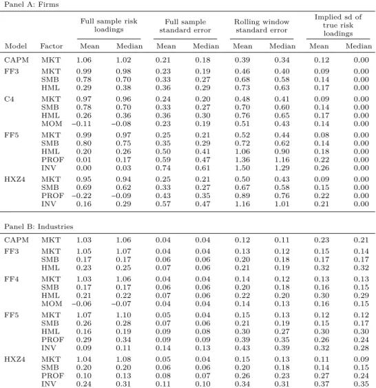
3.4 Estimating Risk Loadings . . . 51
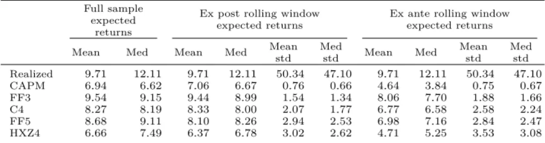
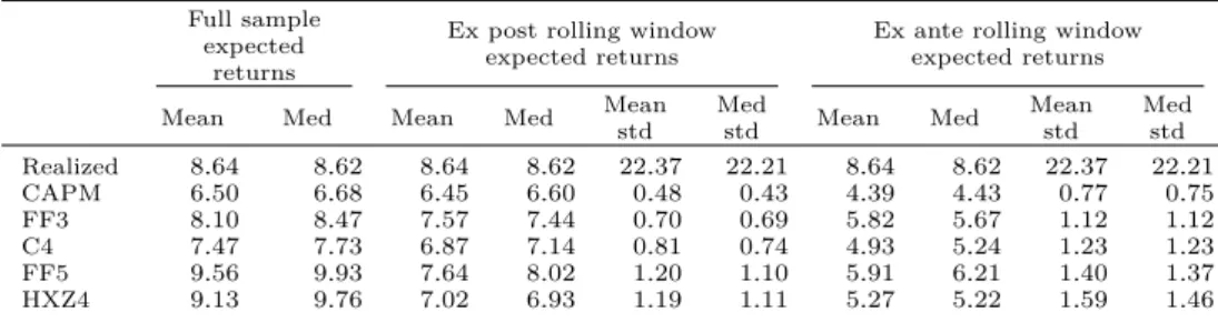
3.5 Estimating Expected Returns . . . 56
3.5.1 Expected Return Point Estimates . . . 56
3.5.2 Model Disagreement . . . 60
3.6 Estimation Error in Expected Returns . . . 62
3.6.1 Standard Errors . . . 62
3.7 Out-of-Sample Forecast Performance . . . 72
3.8 Conclusion . . . 80
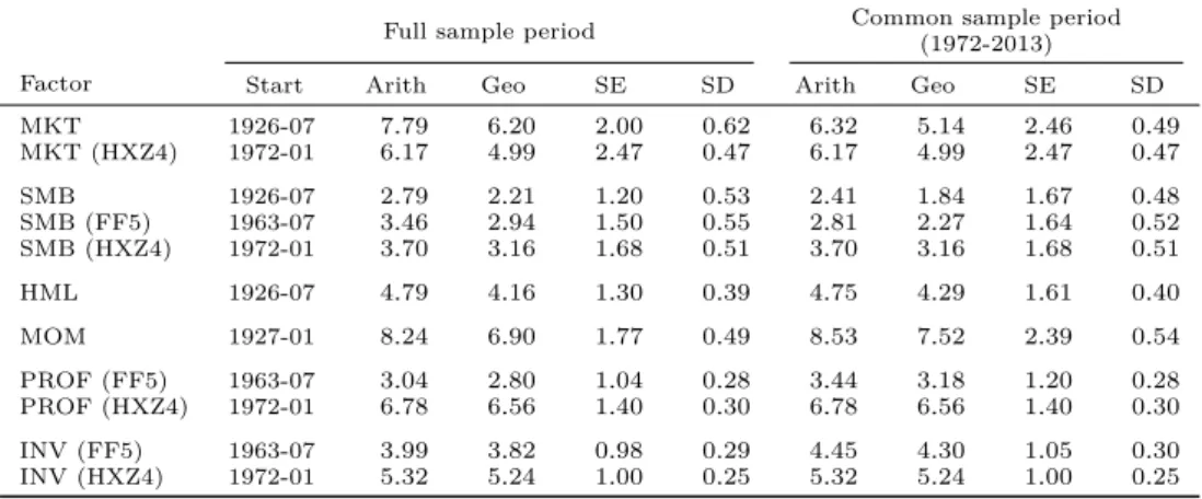
Appendix 3.A Factors . . . 82
Appendix 3.B Factor Construction . . . 83
Appendix 3.C Robustness Checks . . . 86
4 Understanding the Sources of Stock Price Variation 87 4.1 Introduction . . . 87
4.2 Stock Return Decomposition . . . 91
4.2.1 Computing the ICC . . . 92
4.2.2 Cash Flow News and Discount Rate News . . . 93
4.2.3 Industry Return Decomposition . . . 98
4.2.4 Time Series Variation in the Importance of the Sources of Stock Price Variation . . . 100
4.3 Return Decomposition Portfolios . . . 102
4.3.1 Properties of Return Decomposition Portfolios . . . 102
4.3.2 Relation to the Cross-Section of Expected Returns . . . 108
4.3.3 Portfolio Stability Across Time and Investment Horizons . . . . 116
4.4 Predictability of the Equity Premium . . . 119
4.5 Co-Movement in Stock Returns . . . 123
4.6 Conclusion . . . 125
Appendix 4.A Estimating the Implied Cost of Capital . . . 127
Appendix 4.B Discount Rate News and Cash Flow News . . . 130
Appendix 4.C Construction of Firm Characteristic Variables . . . 132
Appendix 4.D Cash Flow and Discount Rate Betas . . . 133
5 Summary and Concluding Remarks 135
Nederlandse Samenvatting (Summary in Dutch) 137
List of Tables
2.1 Frequency Interpretation . . . 14
2.2 Summary Statistics Risk Factors . . . 17
2.3 Correlations Between Risk Factors at Different Horizons . . . 22
2.4 Monthly Cross-Sectional Fama-MacBeth Regressions . . . 25
2.5 Raw and Horizon-Specific Risk Loadings . . . 29
2.6 Cross-Sectional Correlations Between Risk Loadings . . . 31
2.7 Time SeriesR2s . . . 32
2.A.1 Monthly Cross-Sectional Fama-MacBeth Regressions with Shanken Correction . . . 36
2.A.2 Monthly Cross-Sectional Fama-MacBeth Regressions with Haar Filter 37 2.A.3 Monthly Cross-Sectional Fama-MacBeth Regressions with DWT . . . 38
3.1 Risk Premia . . . 50
3.2 Risk Loadings . . . 54
3.3 Realized and Expected Excess Returns for Firms . . . 57
3.4 Realized and Expected Excess Returns for Industries . . . 58
3.5 Standard Errors Expected Returns . . . 63
3.6 Time Series Correlations Standard Errors of Expected Returns . . . . 69
3.7 Statistical Disagreement . . . 70
3.8 Expected Versus Realized Returns for Firms . . . 74
3.9 Expected Versus Realized Returns for Industries . . . 75
3.10 Expected Return Portfolios . . . 79
3.A.1 Overview of Models . . . 82
3.C.1 Expected Versus Realized Returns for Firms with Alternative Risk Loadings . . . 86
4.2 Stock Return Decomposition . . . 95
4.3 Industry Return Decomposition . . . 99
4.4 Characteristics of Return Decomposition Portfolios . . . 103
4.5 Risk Exposures of Return Decomposition Portfolios . . . 106
4.6 Cash Flow and Discount Rate Betas of Return Decomposition Portfolios107 4.7 Pricing of Return Decomposition Portfolios . . . 109
4.8 Return Reversal Portfolios . . . 115
4.9 Cross-Sectional Portfolio Transition Probabilities . . . 117
4.10 Time Series Portfolio Transition Probabilities . . . 118
4.11 Predictive Regressions at Monthly Frequency . . . 121
List of Figures
2.1 Wavelet Decomposition of Risk Factors . . . 20
3.1 Time Series of Expected Return on IBM . . . 42
3.2 Time Series Standard Error of Risk Factor Loadings on Market Factor 67
3.3 Time Series of Standard Errors Expected Returns for Firms . . . 68
3.4 Time Series Differences Expected Returns . . . 71
4.1 Aggregated Return Decomposition . . . 97
4.2 Time Series Variation of Contribution of Return Components . . . . 101
4.3 Time Series Variation in Portfolio Returns . . . 111
Chapter 1
Introduction
This thesis bundles three studies on empirical asset pricing. At its most basic level, the discipline of empirical asset pricing is concerned with the question of why some assets offer higher expected returns than others. The capital asset pricing model (CAPM) by Sharpe (1964), Lintner (1965a,b), and Mossin (1966) is the classical model that provides an answer to this question. In this model, an asset’s expected return is determined by how much it is exposed to one fundamental risk factor: the market factor. An asset that has a large exposure to this factor is risky, because it pays off poorly when the market goes down and pays off well when the market goes up, which leads to high variation in future wealth. To get risk-averse investors to hold this asset, it needs to offer high expected returns as compensation for this undesirable feature. In contrast, an asset that has a low exposure to the market factor is less risky because it is associated with less variation in future wealth. Investors, therefore, accept a lower expected return on such an asset.
Given its intuitive nature and lacking decent alternative models, the CAPM has served as the main workhorse for quite some time. However, early studies already
presented evidence questioning the empirical validity of the CAPM (e.g., Black,
Jensen, and Scholes, 1972; Blume and Friend, 1973; Fama and MacBeth, 1973), which has led to a search for models that better match the empirical patterns in stock prices. Some of these alternative models, and perhaps also those that are most popular, are the Fama and French (1993) three-factor model, the Carhart (1997) four-factor model, the Fama and French (2015) five-factor model, and the Hou, Xue, and Zhang (2015) four-factor model. In fact, scholars have proposed a plethora of factors that are related to the cross-section of expected returns (Harvey, Liu, and Zhu, 2016).
So why do some assets offer higher returns than others? There is no clear-cut answer to this fundamental asset pricing question, and we have to work with models that best fit the data. However, it is not straightforward to pick a model that best fits the empirical properties of asset returns. There are many reasons for this, such as the fact that some models might work well for certain firms or portfolios but not for others (Lewellen, Nagel, and Shanken, 2010). Moreover, estimation error in the risk loadings and risk premia can severely undermine the pricing ability of asset pricing
models (e.g., Fama and French, 1997; Levi and Welch, 2014). The answer also
depends on the investment horizon used to evaluate the models, since some factors might be priced at certain horizons but not at others (e.g., Kamara, Korajczyk, Lou, and Sadka, 2016).
The answer to the fundamental asset pricing question is important to several audiences, although for different reasons. Investors, for instance, might want to un-derstand the exposures of their investments to factors that are empirically associated with a significant price of risk. They might want to use this information to compute expected returns and to form portfolios that match their risk preferences. CFOs and other managers throughout an organization might be interested in knowing why some assets are associated with higher expected returns than others for capital bud-geting purposes. In particular, they need reliable asset pricing models that capture the expected risks many years into the future in order to obtain estimates of the cost of equity capital for net present value (NPV) calculations. Academic researchers are usually interested in identifying how many factors are priced and estimating the corresponding risk premia. This knowledge is used to construct models that explain why asset prices vary in the cross-section and over time. These models are subse-quently used to investigate other important areas within the empirical asset pricing discipline. For instance, models are used to determine whether some investors are able to generate abnormal returns relative to risk-adjusted benchmark returns, and to decompose stock return volatility into a component that captures systematic risk and one that captures idiosyncratic risk.
in the field of empirical asset pricing. Like most studies in this field, the papers are based on US data. Each paper is likely to be of interest to at least one of the previously discussed audiences for which answers to empirical asset pricing questions are important. In particular, Chapter 2 might be of special interest to investors and researchers because it investigates whether risk factors are priced, by how much, and at which investment horizon. Chapter 3 is particularly relevant for CFOs because it discusses whether and how asset pricing models should be used to compute the cost of equity capital. Researchers might be particularly interested in Chapter 4, which enriches our understanding of why stock prices vary, both in the cross-section and time series.
In the second chapter, I study the pricing of systematic risk factors across different horizons. I apply wavelet analysis to extract components of stock returns and widely used risk factors at different horizons and subsequently estimate risk loadings as well as risk premia for each of the horizons separately. I find that the market and size factors are priced at horizons up to sixteen months, while the value, momentum, liquidity, profitability, and investment factors are not priced at any horizon. My results create scope for future research because they leave two open questions. First, future research should focus on providing economic explanations for why certain risk factors are priced at certain horizons and not at others. Second, more research should be directed towards understanding which systematic risk factors are priced into individual stocks as opposed to portfolios.
In the third chapter, I examine whether and how popular asset pricing models can be used by CFOs and other mangers in a firm interested in computing the cost
of equity capital. The cost of equity capital is important because it is used for
NPV calculations and can therefore have a huge impact on valuation and investment decisions. The CAPM has been used for a long time, but given the evidence that the CAPM fails to explain the cross-section of stock returns, and given that many new asset pricing models have been proposed that seem to outperform the CAPM, it is no longer clear which model should be used. I consider (1) the CAPM, (2) the Fama and French (1993) three-factor model, (3) the Carhart (1997) four-factor
model, (4) the Fama and French (2015) five-factor model, and (5) the Hou, Xue, and Zhang (2015) four-factor model, and I study three important aspects of the practical application of these models: (1) model choice, (2) model uncertainty, and (3) model predictability. My main findings are three-fold. My first main finding is that there is considerable disagreement about costs of equity capital across the models. My second main finding is that the cost of equity estimates are often extremely noisy, but even more imprecise when factors get added. My third main finding is that the models have some power in forecasting future stock returns, but only when the cost of equity estimates are relatively precise. Although I cannot say based on the findings which model is best, my results highlight the importance of model selection, but also of estimation error in applying popular asset pricing models. Overall, the results raise questions about the usefulness of asset pricing models and indicate a trade-off between the number of factors and estimation errors. Practitioners should (1) evaluate whether the cost of equity estimates are sensitive to the choice of asset pricing model, and (2) realize that a model is useful only when the cost of equity is estimated relatively precisely.
In the fourth chapter, I examine the drivers of stock price variation. This is a key question because the central aim of asset pricing is to understand why stock prices move. I decompose firm-level stock price variation into a component that captures cash flow news and one that captures discount rate news. I show that there is large cross-sectional heterogeneity in the importance of the two drivers of stock prices at the firm and industry level. This is important, because the sources of stock price variation are associated with different characteristics, risks, and expected returns. The relation to expected returns is intuitive, because if discount rates are stationary, then the stock prices that are predominantly driven by discount rate news should also exhibit stationary behavior. This is as opposed to cash flow news-driven stocks as cash flow news does not need to be stationary. I examine two further applications of the decomposition. First, I examine stock price predictability. Although the forecast errors are large, I show that some macroeconomic variables that are frequently used in prediction models are statistically significant in predicting the returns of cash flow
news-driven stocks, discount rate news-driven stocks, or both. Next, I investigate stock return co-movement and show that stocks driven by discount rate news exhibit more co-movement than stocks driven by cash flow news. These results suggest that it is important to know why asset prices move because answers to other key questions in asset pricing, at least those relating to stock return predictability and return co-movement, are likely to depend on the relative importance of the two components of stock price variation.
In the fifth chapter, I summarize my main findings and present my conclusions. Overall, this thesis explores various areas in the field of empirical asset pricing. It takes us a step, albeit a small one, closer to the answer to the question of why some assets offer higher returns than others. This thesis also provides a sceptical perspective on the field. Chapter 2 points to the limited ability of popular asset pricing models to explain the cross-section of individual stock returns, and Chapter 3 casts serious doubts on their usefulness for capital budgeting. In future research, my aim is to provide more guidance to investors, managers, and researchers in making investment and corporate finance decisions, and increase our understanding of how financial markets function.
Declaration of Contribution
Chapter 2 is joint work with Marta Szymanowska and Mathijs van Dijk. Together we developed the research idea. I have collected the data and executed the analysis. We have jointly written this chapter. Thomas Conlon and Andrea Tamoni provided us with helpful suggestions.
Chapter 3 is single-authored work, which greatly benefited from feedback from Marta Szymanowska and Mathijs van Dijk. I also received useful comments and sug-gestions from Dion Bongaerts, Mathijs Cosemans, Pascal François, Bruno Gérard, Rogier Hanselaar, Espen Henriksen, Xavier Mouchette (discussant), Laurens Swinkels, Wolf Wagner, Darya Yuferova, and seminar participants at Erasmus University, Nor-wegian School of Management (BI), and the 33rd International Conference of the French Finance Association.
Chapter 4 is single-authored work. I received valuable feedback from Marta Szy-manowska and Mathijs van Dijk, as well as useful comments and suggestions from Dion Bongaerts, Mathijs Cosemans, and Rogier Hanselaar.
Chapter 2
The Pricing of Systematic Risk Factors Across
Hori-zons
∗2.1
Introduction
By now, the conclusion that the classical CAPM fails to explain the cross-section of stock returns is widely accepted. In response to this conclusion, the asset pricing literature has proposed a number of multi-factor asset pricing models that contain additional systematic risk factors. These models include the Fama and French (1993) three-factor model, the Carhart (1997) four-factor model (occasionally augmented with the Pastor and Stambaugh (2003) liquidity factor), and the Fama and French (2015) five-factor model. Despite the popularity of these models, there is an ongoing debate on which risk factors included in these models are priced, and which of these models works better.
An important question that has received relatively little attention to date concerns the horizon over which risks are priced. The common approach in the empirical asset pricing literature is to study monthly returns and estimate Fama and MacBeth (1973) cross-sectional regressions to determine average risk premia associated with different factors. This approach does not allow the risk premium of any factor to be horizon-dependent. Theoretically, Beber, Driessen, and Tuijp (2012) and Brennan and Zhang (2016) develop asset pricing models in which investors have stochastic or heterogeneous horizons, and show that there are important horizon effects in the pricing of risks in such settings.
The question of whether risk premia differ across horizons is important for at least
∗This chapter is based on Szymanowska, Van Dijk, and Verbeek (2017) “The Pricing of
System-atic Risk Factors Across Horizons.” We thank Thomas Conlon and Andrea Tamoni for providing us with helpful suggestions.
two reasons. First, from an academic perspective a true understanding of the nature of asset pricing requires an understanding of the horizon over which economic risks manifest and of the risk premia investors demand as compensation for risks materi-alizing at different horizons. Second, from the perspective of capital budgeting, it is important to study how to discount future cash flows arriving at different horizons. If risk premia depend on the horizon, discounting a stream of future cash flows arriving at different horizons requires a term structure of risk premia, analogous to the term structure of discount rates obtained from discount bonds.
In this paper, we use wavelet analysis to study the relation between risk and return at different horizons. Wavelet analysis is a method that decomposes a time series into components that capture patterns associated with specific time horizons. When applied to risk factors, this method allows us to separate factor risks across horizons. In particular, we decompose the returns on risk factors as well as the excess returns on a set of test assets into five components that are associated with horizons of two to four months, four to eight months, eight to sixteen months, sixteen to 32 months, and 32 to 64 months. Our empirical analysis is based on seven different factors included in the CAPM, the Fama and French (1993) three-factor model, the Carhart (1997) four-factor model augmented with the Pastor and Stambaugh (2003) liquidity factor, and the Fama and French (2015) five-factor model. These factors are the market (MKT), size (SMB), value (HML), momentum (WML), liquidity (LIQ), profitability (RMW), and investment (CMA) factors.
We first show that the decomposition of the factor returns produces components of the risk factors that differ dramatically in their persistence and smoothness. The
short-horizon components are very jumpy and highly mean-reverting. The
long-horizon components are much more smooth and persistent, indicating that the signals are de-noised, such that events like the bursting of the internet bubble become more apparent than in the non-decomposed, raw factor returns.
We subsequently estimate the risk loadings of the test assets with respect to the factor components at each individual horizon by running time series regressions of the asset return components on the corresponding factor components. The risk loading
that is estimated at a short (long) horizon captures the sensitivity of high (low) frequency fluctuations in excess returns to high (low) frequency fluctuations in factor returns. We proceed by evaluating the risk premia associated with the risk loadings at different horizons based on Fama and MacBeth (1973) regressions estimated at each horizon separately, thus deriving a term structure of systematic risk premia. Our sample period is from January 1968 to December 2015. We start in January 1968 because the Pastor and Stambaugh (2003) traded liquidity factor is available from that time.
As pointed out by, for instance, Lewellen, Nagel, and Shanken (2010), the choice of test assets is very important in asset pricing tests. We use random portfolios as our test assets and construct them by sorting individual stocks randomly into 1,000 monthly-rebalanced portfolios in which each stock has an equal weight. We use ran-dom portfolios instead of firms to circumvent the problem of missing observations in individual stock return data. This is important, because the wavelet decomposition requires an uninterrupted time series of returns. As shown by Ecker (2013), using random portfolios yields similar Fama and MacBeth (1973) cross-sectional results as using firms. He also shows that one major benefit of using random portfolios is the significant reduction in the measurement errors in the risk loadings, which is one of the main motivations for forming portfolios in the first place. Moreover, the risk premium estimates based on random portfolios are insensitive to the choice be-tween constant and time-varying risk loadings because either type yields qualitatively similar results.
Although we could restrict our sample to firms for which we have an uninterrupted time series of return data, we do not because this would result in a non-representative sample that is heavily biased towards old and stable firms. We also do not use characteristic-sorted portfolios, such as the classic Fama and French (1993) portfolios sorted on size and book-to-market ratio, because it is well-known that risk premium estimates are very sensitive to the choice of test assets (Lewellen, Nagel, and Shanken, 2010; Ahn, Conrad, and Dittmar, 2013; Ecker, 2013). Intuitively, using portfolios that are sorted on a characteristic (such as size) that forms the basis of one of the
risk factors (such as SMB) as test assets tends to “favor” that factor in asset pricing tests. Another unattractive feature of characteristic-sorted portfolios is that the risk premium estimates based on Fama and MacBeth (1973) cross-sectional regressions are very sensitive to the choice of using the full sample or a rolling window to estimate the risk loadings (Ecker, 2013).
Our results point to important horizon effects in the pricing of systematic risk. We find that the market and size factors are priced when monthly, raw (non-decomposed) returns are used. Across horizons, we find that these two factors are priced up to six-teen months. In contrast, we find that the value, momentum, liquidity, profitability, and investment factors are not priced at any horizon. This finding is consistent with the literature that generally finds weak firm-level pricing results on risk factors (e.g., Daniel and Titman, 1997; Ecker, 2013; Kamara, Korajczyk, Lou, and Sadka, 2016). Our results show that these factors are also not priced across any of the horizons that we consider.
The study that is probably closest to ours is Kamara, Korajczyk, Lou, and Sadka (2016). They assess the pricing of different factors over different horizons by measur-ing test asset as well as factor returns over different horizons rangmeasur-ing from one month up to five years, in the spirit of Handa, Kothari, and Wasley (1989) and Jagannathan and Wang (1996). However, their horizon-specific pricing results are different from ours. They find no factors to be priced at the monthly horizon and some factors to be priced at longer horizons. In particular, they find that liquidity risk is priced at a three- to six-month-horizon, that market risk is priced at a six- to twelve-month-horizon, and that the value factor is priced at a two- to three-year horizon. They do not find a significant premium for the size and momentum factor at any horizon.
Although their analysis is interesting and insightful, we believe that our appli-cation of wavelet analysis to analyze the pricing of systematic risk factors forms a significant contribution to their study. There are two reasons for this. First, Valkanov (2003) demonstrates that long-horizon regressions, in which the variables are based on a rolling summation of the original time series, can produce significant results irrespective of there being a true structural relation between the variables. Second,
an important advantage of wavelet analysis is that it allows us to really separate out short-term versus long-term fluctuations, while compounding returns over different horizons leads to the inclusion of both short-term and long-term fluctuations. Sep-arating out the short- and long-term components of various risk factors enables us to study the importance of low- and high-frequency manifestations of the different systematic risk factors, and the extent to which investors want to be compensated for each of these separate risks.
Our study contributes to a discussion in the literature on whether the term struc-ture of equity risk premia is upward-sloping, flat, or downward-sloping. Most the-oretical models imply that the term structure is either flat or upward-sloping (e.g., Campbell and Cochrane, 1999; Bansal and Yaron, 2004; Barro, 2006; Goyal, 2012). Empirically, however, there is evidence that the term structure is downward-sloping (e.g., Van Binsbergen, Brandt, and Koijen, 2012; Weber, 2017). Our study adds to this discussion because our results indicate, contrary to the theoretical predictions and recent empirical findings, that the term structure of the equity premium seems to be non-linear. In fact, we find an upward-sloping term structure of the market factor up to sixteen months, and at longer horizons we find the risk premium to be insignificant. For the size factor we find a term structure that is similarly shaped.
We add to this discussion by taking an approach that does not suffer from the criticisms raised against using dividend strips, which are usually used to study the term structure of the equity premium (Van Binsbergen, Brandt, and Koijen, 2012). In particular, one drawback of using strips is that the results might be driven by microstructure noise (Boguth, Carlson, Fisher, and Simutin, 2012). Another contri-bution that we make to this literature is that we not only examine the term structure of market risk, but also that of other risk factors. In addition, we employ the entire cross-section in CRSP and cover an extensive sample period (from 1968 until 2015), while the studies that use dividend strips are based on a much smaller cross-section and cover a shorter period of time.
Our study also contributes to the small but growing body of finance research that applies wavelet analysis to the field of asset pricing. We add to studies that
focus on the estimation of risk loadings at different horizons (Gençay, Selçuk, and Whitcher, 2003; In and Kim, 2006; Gençay, Selçuk, and Whitcher, 2007; Trimech, Kortas, Benammou, and Benammou, 2009; In and Kim, 2013) by instead focusing on the estimated risk premia at different horizons. In addition, while this literature mainly studies the CAPM market factor, and sporadically also the Fama and French (1993) size and value factors and the Carhart (1997) momentum factor, we examine other factors as well. Moreover, while this literature usually considers a small and specific set of test assets, we consider the full CRSP file. The literature has also used wavelet analysis to relate risk factors to innovations in state variables (In and Kim, 2007), and to study other macroeconomic variables, such as consumption growth, on a horizon-by-horizon basis (Ortu, Tamoni, and Tebaldi, 2013; Bandi and Tamoni, 2017). However, to the best of our knowledge, our study is the first to apply wavelet analysis to the study of the pricing of systematic risk factors from several widely used multi-factor asset pricing models at different horizons.
2.2
The Relation Between Risk and Return Across Different
Horizons
In this paper, we are interested in studying the relation between risk and return at different horizons. Traditionally, this relation is evaluated using the Fama and MacBeth (1973) cross-sectional regression approach where loadings to risk factors and prices of risk are estimated using the time series and cross-section of excess returns on test assets and factors. In this section, we describe how we perform this analysis on a horizon-by-horizon basis. This allows us to assess whether risk factors we analyze are particularly relevant at certain horizons. To compute horizon-specific risk loadings and prices of risk, we use the wavelet approach to decompose the time series of excess returns on the test assets and factors across different horizons. Subsequently, we estimate horizon-specific loadings and prices of risk using the components. We explain our method in detail below.
2.2.1 Wavelet Decomposition
We use wavelet decomposition because it allows us to truly separate out the con-tribution to risk of distinct horizons from our time series. In particular, our decom-position allows us to study long-horizon effects that are distinct from short-horizon fluctuations. This approach is fundamentally different from examining horizon effects by first aggregating the returns on test assets and factors over particular horizons and then resorting to the traditional Fama and MacBeth (1973) approach (e.g., Ka-mara, Korajczyk, Lou, and Sadka, 2016). In this subsection, we outline the basic concepts of the wavelet transform we use. We refer the reader to Gençay, Selçuk, and Whitcher (2002) and In and Kim (2013) for a more extensive discussion of ap-plications of wavelet analysis in finance and economics.
To decompose the time series of excess returns on our test assets and factors, we use the maximum overlap discrete wavelet transform (MODWT) with the Daubechies (1992) least asymmetric filter with eight lags (LA8). We choose MODWT mainly because of its ability to handle any sample size, increased resolution at longer hori-zons, and because it is a more asymptotically-efficient variance estimator than the alternative DWT. We use the LA8 filter because it is much closer to an ideal band-pass filter than the Haar filter (Gençay, Selçuk, and Whitcher, 2003). In robustness tests, we find similar results with the DWT and Haar filter.
Wavelet analysis is different from the more classical spectral analysis tools, which are also used to study market dynamics across investment horizons (e.g., Chaud-huri and Lo, 2016). Spectral analysis is used to describe a time series process as a function of frequency. While spectral analysis does not have a time dimension, the wavelet transform preserves information both in time and frequency. In contrast to wavelets, spectral analysis assumes stationarity and regular periodicity in the time series. Those assumptions are often not reasonable for financial data.
Our wavelet decomposition separates a time series xxx of length T, which could
combination ofJ components with different frequencies (or time horizons): xxx= J Õ j=1 f Wj0wweewej+VeJ0eeevvvJ (2.1)
wherewweeewj is a vector containing the wavelet coefficients,eeevvvJ is a vector containing the
scaling coefficients, andWfandVeare matrices that define the MODWT. The wavelet
coefficients capture innovations inxxx at horizons that correspond to time intervals of [2j,2j+1]for j <J. The scaling coefficients capture the long-term trend in xxx, which
is determined by the sample average over horizons of more than 2J periods. The
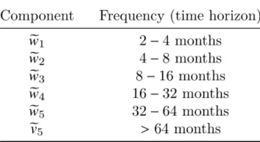
frequency interpretation for these components is summarized in Table 2.1.
Table 2.1. Frequency Interpretation
Component Frequency (time horizon)
e w1 2−4 months e w2 4−8 months e w3 8−16months e w4 16−32months e w5 32−64months ev5 >64months
In our main analysis, we use five components. This choice reflects a trade-off between understanding the risk-return relation at longer horizons and the exclusion of observations as a result of boundary conditions. Boundary conditions play an
important role when the time series xxx has finite length. Since we do not want to
make unrealistic assumptions about boundary conditions, we remove their effect by ignoring the first(L−1)(2j−1)observations for every component in
e
wewwej, whereLis the length of the wavelet filter. Excluding observations is problematic because it leads to more estimation error in the risk loadings and, consequently, in the risk premia. Extracting five components results in the exclusion of7× (25−1)=217observations in the fifth component due to boundary conditions. Extracting six components would result in the exclusion of7× (26−1)=441observations in the longest term wavelet coefficient, which amounts to almost all observations. Our choice to extract five components is consistent with the literature in which usually four to six components
are extracted (e.g., Gençay, Selçuk, and Whitcher, 2003; In and Kim, 2006; Trimech, Kortas, Benammou, and Benammou, 2009; In and Kim, 2013; Ortu, Tamoni, and Tebaldi, 2013).
2.2.2 Horizon-Specific Risks
Following, among others, Gençay, Selçuk, and Whitcher (2003), In and Kim (2013), Boons and Tamoni (2015), and Bandi and Tamoni (2017), we evaluate the risk-return relation over different horizons using the wavelet coefficients defined above. An important characteristic of our wavelet transform is its ability to decom-pose the variance of a time series as well as the covariance between two time series. Therefore, we can define the horizon-specific factor loading as:
β(j) i =
Cov(Ri(j),t,Ft(j)) Var(Ft(j))
(2.2)
where R(j)i,t is the jth component of excess returns on asset i, and Ft(j) is the vector
with the jth components of the returns on the factors. We estimate those loadings
in the following regression, using components of returns on assets and factors:
Ri(,jt)=αi(j)+FFF(tj)0βββi(j)+εi(,jt),forj =1,2, ...,J (2.3) Thus,ˆβββ(j)i measures the horizon-specific loadings of a security on the risk factors.
Next, we assess whether the horizon-specific risk loadings capture cross-sectional variation in asset returns by running the following Fama and MacBeth (1973) cross-sectional regression at each point in time:
Ri,t=Λ(j)0 +βββˆ (j)0 i ΛΛΛ (j) t +u (j) i,t,forj=1,2, ...,J (2.4) Note that we use non-decomposed returns as the dependent variable, because we are interested in how factor loadings (here estimated across different horizons) are related to expected returns. We do not use the return components as the dependent variable because our method allows us to decompose return variance, not return levels. We
estimate the risk premia at horizon j byΛΛΛ¯(j) = 1 T
ÍT−1
t=0 ΛΛΛˆ
(j)
t . Thus, horizon effects
might not only show up in the risk loadings, but also in the estimated risk premia. This empirical decomposition can be motivated by recent theoretical models. For instance, Brennan and Zhang (2016) examine a model in which investors have a stochastic investment horizon and returns are serially dependent. They show that, in this setting, expected returns are a weighted sum of horizon-specific risk loadings times the corresponding market risk premia. This is contrary to the fixed-horizon CAPM that assumes the risk loadings and risk premium to be horizon-invariant. Our wavelet decomposition leads to a similar representation of expected returns as in Brennan and Zhang (2016) because it gives us horizon-specific risk loadings and risk premia per factor. Hence we extend their set-up by examining the horizon effects that are present in multiple risk factors as opposed to only the market factor.
2.3
Risk Factors Across Horizons
We retrieve the factors included in the CAPM, the Fama and French (1993) three-factor model, the Carhart (1997) four-three-factor model, and the Fama and French (2015)
five-factor model, and the risk-free rate from Ken French‘s Data Library.1 We obtain
the Pastor and Stambaugh (2003) traded liquidity factor from WRDS.
We present summary statistics on the decomposition of the risk factors in Ta-ble 2.2. Specifically, we report the mean and variance of the monthly factor returns,
and the (relative) wavelet energies. As shown in Gençay, Selçuk, and Whitcher
(2003), our wavelet transformation preserves the variance of the original time series, and thus we can decompose the variance in the following way:
kxxxk2= J Õ j=1 wweewej 2 + eevvevJ 2 (2.5)
wherekxxxk2is the variance of the time seriesxxx,wweeewj
2
captures the energy from changes at horizon j andeeevvvJ
2
captures the energy from the residual, long-term component. This equation shows that the variance decomposition allows us to determine whether
1We thank Ken French for making the data available at:
T able 2.2. Summary Statistics Risk F actors This table presen ts summary sta tistics on the decomp osition of sev en risk factors. T h e risk factors used are the mark et (MKT), siz e (SMB), v alue (HML), momen tum (WML), liquidit y (LIQ), profitabil it y (RMW), and in v estmen t (CMA) factors. The momen tum factor is from Carhart (1997), the liquidit y factor is the tra d e d liquidit y factor from P astor and Stam baugh (2003), and the remaining factors are from the F ama and F renc h (2 015) fiv e-factor mo del. W e apply the maxim um o v erlap discrete w a v elet tra n sform (MOD WT) based on the least asymmetr ic Daub ec hies (1992) w a v elet filter with eigh t lags (LA8) to the risk factors. W e exclude 7 × ( 2 j− 1 ) observ ations at the b eginning of the resulting time series to remo v e an y effect of b oundary conditions. In total w e ex tract six comp onen ts. W e presen t the a v erage (A vg), v ariance (V ar), scaled sum of squared w a v elet co efficien t v ect ors (Energies), a n d energies as a fracti on of the summed energies of all factor comp onen ts (Relativ e En e rgies). Energies are calculated for w a v elet co efficien ts 1 to 6 ( e w1 to e w6 ). The energies are scaled b y N 2 − j for comparison purp oses. The samp le p erio d is from Jan uary 1968 to Decem b er 2015. Energies Relati v e Energies F actor A vg V ar e w1 e w2 e w3 e w4 e w5 e w6 e w1 e w2 e w3 e w4 e w5 e w6 MKT 0 . 48 20 . 87 18 . 77 21 . 70 21 . 50 20 . 33 11 . 85 2 . 14 0 . 19 0 . 22 0 . 22 0 . 21 0 . 12 0 . 02 SMB 0 . 19 9 . 44 8 . 62 9 . 88 9 . 68 6 . 26 3 . 98 2 . 06 0 . 21 0 . 24 0 . 23 0 . 15 0 . 10 0 . 05 HML 0 . 36 8 . 36 6 . 69 8 . 22 10 . 03 8 . 98 14 . 19 2 . 11 0 . 13 0 . 16 0 . 20 0 . 18 0 . 28 0 . 04 WML 0 . 68 18 . 95 17 . 32 20 . 44 18 . 25 20 . 10 9 . 91 1 . 57 0 . 20 0 . 23 0 . 21 0 . 23 0 . 11 0 . 02 LIQ 0 . 42 12 . 29 10 . 89 13 . 70 16 . 48 6 . 04 7 . 14 1 . 14 0 . 19 0 . 23 0 . 28 0 . 10 0 . 12 0 . 02 RMW 0 . 26 5 . 33 4 . 30 5 . 73 5 . 79 5 . 38 9 . 02 0 . 84 0 . 14 0 . 18 0 . 19 0 . 17 0 . 29 0 . 03 CMA 0 . 35 4 . 09 3 . 42 3 . 66 4 . 81 3 . 54 3 . 47 1 . 04 0 . 16 0 . 17 0 . 23 0 . 17 0 . 17 0 . 05
most energy is captured by either the short- or long-term components, or whether it is equally distributed across all components of the original time series.
The first two columns of Table 2.2 indicate that there are considerable differences across the factors in terms of their average returns and variances. Momentum clearly
dominates in terms of average return, with a factor realization of0.68% per month.
On the other end, the size factor delivers the smallest return of only0.19%per month. We see more variation across factors in terms of their variance. Momentum together with the market factor have the highest variance, while the variance of the more recently proposed profitability and investments factors is four times smaller.
In the remaining columns we examine the horizon-specific components of the factors by looking at their energy decomposition across horizons. The results for the absolute and relative wavelet energies show that the differences in scaled energies across horizons are relatively minor at the short and intermediate horizons, and that the energies are substantially lower at the long-term horizons. The sixth component of all factors exhibits virtually no variation over time, suggesting that estimating risk loadings at the corresponding horizon is problematic. This prompted us to decide to focus on the first five components. We also note that there are some minor differences in the energy distributions across factors. For example, the size and liquidity factors have slightly more energy contained at shorter horizons, while the value, profitability, and investment factors slightly dominate at longer horizons.
Using a different methodology, Kamara, Korajczyk, Lou, and Sadka (2016) also analyze the importance of risks at different horizons. They examine the variance ratios of the risk factors by using continuously compounded returns over varying horizons. This is different from our approach because their long-horizon factors also include short-term effects while our decomposition separates the two. They find that liquidity risk is greater in the short-term as the liquidity factor has negative serial correlation, and that value risk is greater in the long term because it has positive
serial correlation.2 They do not find evidence suggesting that market, size, and
momentum risk is greater at particular horizons. Thus, our results are largely in line
2We note that Kamara, Korajczyk, Lou, and Sadka (2016) use the non-traded liquidity factor of
with Kamara, Korajczyk, Lou, and Sadka (2016).
To illustrate how the decomposition works and to show that it reveals insights into the dynamics of factor returns, we plot the evolution of the factor returns and their components in Figure 2.1. In each figure, the raw return series is presented first, followed by the wavelet coefficients. Note that the first7× (2j−1)observations are excluded because they are affected by boundary conditions. The components are circularly shifted to align them better with the raw data in calendar time (Gençay, Selçuk, and Whitcher, 2003).
The figure clearly shows that the wavelet coefficients become smoother for the components that capture variation over increasingly longer horizons. One interpre-tation of the series becoming smoother for longer horizons is that the signals are de-noised, since short-term fluctuations are filtered out. The coefficients that cap-ture variation at longer horizons are able to identify events that might be obscured in the raw series or the short-horizon components. For example, the fifth wavelet coefficient of the market factor clearly identifies the bursting of the internet bubble in 2001 and the global financial crisis in 2007 and 2008. The coefficients also re-veal a size crash in 1998, a momentum crash in 2009 (Daniel and Moskowitz, 2016), and a spike in the liquidity and profitability factors around 2001. By comparison, these events are harder to detect in the raw data series or one of the short-term components. Hence, all components capture an important part of the variation in our original series, and the differences between the components allow us to focus on horizon-specific dynamics that may be obscured in the aggregate series.
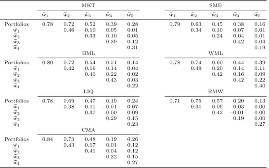
Given the relative smoothness of the longest-horizon components of each of the factors, one concern could be that the long-horizon components of several differ-ent risk factors capture the same underlying long-term trend. We therefore analyze whether our decomposition affects the correlation structure between the factors. Ta-ble 2.3 presents correlations between the factors, estimated for the raw series as well as the components.
In general, the magnitudes of the correlation coefficients vary only slightly across the components, and the statistical significance decreases with the increasing horizon
Table 2.3. Correlations Between Risk Factors at Different Horizons
This table presents Pearson correlations and wavelet correlations between seven risk factors. The risk factors used are the market (MKT), size (SMB), value (HML), momentum (WML), liquidity (LIQ), prof-itability (RMW), and investment (CMA) factors. The momentum factor is from Carhart (1997), the liquidity factor is the traded liquidity factor from Pastor and Stambaugh (2003), and the remaining fac-tors are from the Fama and French (2015) five-factor model. We apply the maximum overlap discrete wavelet transform (MODWT) based on the least asymmetric Daubechies (1992) wavelet filter with eight lags (LA8) to the risk factors. We exclude7× (2j−1)observations at the beginning of the resulting time
series to remove any effect of boundary conditions. In total we extract five components. Results are presented for the non-decomposed series (Raw), and wavelet coefficients 1 to 5 (we1towe5). The sample
period is from January 1968 to December 2015. *, **, and *** indicate significance levels of10%,5%, and1%, respectively. SMB HML WML LIQ RMW CMA Raw MKT 0.26*** −0.28*** −0.14*** −0.07 −0.24*** −0.40*** e w1 0.10 −0.31*** −0.07 −0.09 −0.22*** −0.40*** e w2 0.38*** −0.25*** −0.21** −0.02 −0.25*** −0.37*** e w3 0.62*** −0.21* −0.21* 0.05 −0.25** −0.41*** e w4 0.44*** −0.30* −0.22 −0.14 −0.40** −0.43*** e w5 0.24 −0.45* 0.13 −0.39 −0.50** −0.26 Raw SMB −0.10** −0.04 −0.02 −0.37*** −0.08** e w1 −0.08 0.00 −0.03 −0.45*** −0.03 e w2 −0.17** −0.09 −0.02 −0.48*** −0.16* e w3 −0.10 −0.11 −0.12 −0.23** −0.22* e w4 −0.24 0.05 0.17 −0.38** −0.21 e w5 0.15 −0.05 −0.26 0.00 0.13 Raw HML −0.18*** 0.01 0.10** 0.70*** e w1 −0.12** 0.12** 0.13** 0.69*** e w2 −0.19** −0.05 0.13 0.67*** e w3 −0.27** −0.18 −0.13 0.75*** e w4 −0.24 0.18 0.35** 0.73*** e w5 −0.31 0.16 0.64*** 0.72*** Raw WML −0.01 0.11** 0.01 e w1 −0.11* 0.14** 0.05 e w2 0.08 0.16* 0.03 e w3 0.05 0.01 0.07 e w4 −0.08 −0.04 0.03 e w5 −0.09 −0.06 −0.28 Raw LIQ 0.03 0.02 e w1 0.03 0.08 e w2 −0.04 0.00 e w3 0.07 −0.12 e w4 0.03 0.22 e w5 0.37 −0.09 Raw RMW −0.01 e w1 0.00 e w2 0.02 e w3 −0.11 e w4 0.21 e w5 0.28
due to the relatively larger estimation errors as a result of a smaller number of inde-pendent observations that are available for the long-term components. We conclude that, although there is variation in the correlation coefficients across horizons, the correlation structure between the factors is largely preserved by the decomposition. This is important for our subsequent analyses of the loadings and prices of risk across different horizons.
2.4
The Pricing of Risk Across Horizons
We now turn to our main analysis of the risk-return trade-off across different horizons. To this end, we study whether horizon-specific loadings can explain cross-sectional variation in our test asset returns and whether their explanatory power varies with the horizon.
Our test assets are randomly generated portfolios based on individual firms. Al-though the risk premium estimates based on random portfolios are very similar to those based on individual firms (Ecker, 2013), there are some important advantages to using random portfolios. One of them is that random portfolios provide an un-interrupted time series of return data, which our decomposition method requires. Another benefit of random portfolios is that the risk loadings are relatively precisely estimated, and that the results are insensitive to whether the risk loadings are esti-mated on the full-sample or on a rolling window basis. Rolling window risk loadings are often used instead of full sample risk loadings to capture a firm’s changing risk profile over time. However, since the expected risk profile of each portfolio is reset to the cross-sectional average risk profile every month, there is no reason to expect that using rolling window risk loadings yields different pricing results than using full sample risk loadings. In our analysis, we use 1,000 monthly-rebalanced random port-folios and compute equally-weighted returns. As shown in Ecker (2013), the Fama and MacBeth (1973) regression results are not sensitive to the number of portfolios. We use equal and not value weighting so as not to undermine the comparability with the standard firm-level Fama and MacBeth (1973) results.
We retrieve monthly stock return data from CRSP. We use ordinary common shares (share codes 10 and 11) that are listed on the NYSE, AMEX, and NASDAQ
(exchange codes 1, 2, and 3). We require prices to be at least $1, and we also require at least 24 return observations to be available for a firm to be included in the sample. We impose this restriction in order to obtain full-sample firm-level risk loading estimates that are reasonably precise. The sample period starts in January 1968 and ends in December 2015.
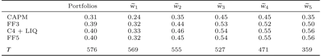
Table 2.4 reports annualized average risk premium estimates based on both
non-normalized and non-normalized risk loadings,t-statistics, and averageR2s from running
cross-sectional Fama and MacBeth (1973) regressions of our test asset returns on
horizon-specific loadings for all four models.3 We present risk premium estimates
based on normalized risk loadings for comparison purposes. This is necessary because, as we show later, there are large differences in the distribution of risk loadings across horizons and risk factors. We normalize by setting the cross-sectional variance of the risk loadings to unity.
We first examine the risk premium estimates for individual firms based on raw
data and compare them with those based on random portfolios. Examining the
risk premium estimates based on individual firms, we find that the market and size factors have significant prices of risk in all factor models. The corresponding Newey and West (1987)t-statistics are around2.0for both factors. We do not find significant prices of risk related to the value, momentum, liquidity, profitability, and investment factors in any of our specifications. These weak pricing results based on individual firms are consistent with the literature. For instance, Kamara, Korajczyk, Lou, and Sadka (2016) use rolling window risk loadings and do not find any factor to be priced at the monthly horizon. Ecker (2013) uses full-sample risk loadings and finds, like us, the market and size factors to be priced. We note that most studies that find the other factors to be priced (e.g., Fama and French, 2015) use characteristic-sorted portfolios instead of individual firms as test assets.4
3Since the risk loadings must be estimated, one might be concerned about the errors-in-variables
(EIV) problem. To alleviate this concern, we also estimate Shanken (1992)t-statistics and report the results in Appendix 2.A. Our main conclusions do not change with these alternativet-statistics.
4In fact, we have tried various characteristic-sorted portfolios from Ken French’s Data Library,
among others. In line with the findings in the literature, we find that the pricing results are very sensitive to the choice of test assets. It is not uncommon to find that some factors have positive significant risk premium estimates when using one set of test assets and negative significant estimates when using another. Often, we find factors to be priced when the variable on which the factor is
T able 2.4. Mon thly Cross-Sectional F ama-MacBeth Regressi ons This table presen ts results from cross-sectional F ama and MacBeth (1973) regr ess ions based on ra w and horizon-sp ecific risk loadings. The p ortfolio returns are from 1,000 random p ortfolios. W e use the CA PM, the F ama and F renc h (1993) three-factor mo del, the Carhart (1997) four-factor mo del augmen ted with the P astor and Stam baugh (2003) traded liquidit y factor, and the F ama and F renc h (2015) fiv e-factor mo del. The fac tors used are the mark et (MKT), size (SMB), v alue (HML), momen tum (WML), liquidit y (LIQ), profitabilit y (RMW), and in v estmen t (CMA) factors. W e apply the maxim um o v erlap discrete w a v elet transform (MOD WT) based on t h e least asymmetric Daub ec hies (1992) w a v elet filter with eigh t lags (LA8) to the p ortfolio excess returns and risk factors. W e exclude 7 × ( 2 j− 1 ) observ ations at the b eginning of the resulting time series to remo v e an y effect of b oundary conditions. In total w e e xtract fiv e comp onen ts. W e obtain full sample risk loadings on a horizon-b y-horizon basis and run cross-sect ional F ama and MacBeth (1973) regressions. W e rep ort ann ualized risk premium estimates based on non-normalized and normalized risk loadings, corresp onding F a ma and MacBeth (1973) t -statistics with New ey and W est (1987) adju stme n t, and a v erage cross-sectional R 2s. Results are presen ted for risk loadings that corr esp ond to aggregate risk loadings (Firms and P ortf.), and horizon-b y-horizon risk loadings ( e w1 to e w5 ). The sample p erio d is from Jan uary 1968 to Decem b er 2015. W e presen t a v erage results b a s e d on 100 indep enden t sim ulation runs. CAPM F F3 C4 + LIQ FF5 MKT R 2 MKT SMB HML R 2 MKT SMB HML WML LIQ R 2 MKT SMB HML RMW CMA R 2 Risk premia Firms 6 . 66 3 . 20 5 . 73 3 . 29 − 2 . 11 6 . 91 5 . 41 3 . 15 − 1 . 94 1 . 22 − 0 . 84 9 . 28 5 . 42 3 . 21 − 2 . 03 − 1 . 56 − 0 . 79 9 . 42 Non-norm. P ortf. 6 . 97 0 . 36 5 . 75 4 . 58 − 1 . 73 1 . 03 5 . 24 4 . 51 − 1 . 88 − 2 . 02 − 1 . 08 1 . 60 5 . 78 4 . 48 − 1 . 54 − 1 . 92 − 0 . 82 1 . 66 Risk premia P ortf. 0 . 58 0 . 36 0 . 50 0 . 69 − 0 . 27 1 . 03 0 . 44 0 . 67 − 0 . 29 − 0 . 23 − 0 . 11 1 . 60 0 . 52 0 . 65 − 0 . 31 − 0 . 42 − 0 . 22 1 . 66 Normalize d e w1 0 . 33 0 . 33 0 . 32 0 . 42 − 0 . 22 0 . 95 0 . 30 0 . 42 − 0 . 21 − 0 . 18 − 0 . 05 1 . 53 0 . 31 0 . 39 − 0 . 18 − 0 . 45 − 0 . 20 1 . 54 e w2 0 . 49 0 . 32 0 . 50 0 . 59 − 0 . 21 0 . 95 0 . 49 0 . 60 − 0 . 21 − 0 . 05 − 0 . 07 1 . 51 0 . 51 0 . 60 − 0 . 27 − 0 . 34 − 0 . 26 1 . 55 e w3 0 . 55 0 . 30 0 . 65 0 . 68 − 0 . 22 0 . 88 0 . 65 0 . 69 − 0 . 23 − 0 . 06 − 0 . 13 1 . 43 0 . 61 0 . 66 − 0 . 26 − 0 . 40 − 0 . 28 1 . 46 e w4 0 . 43 0 . 29 0 . 50 0 . 15 − 0 . 31 0 . 85 0 . 45 0 . 17 − 0 . 32 − 0 . 24 − 0 . 12 1 . 39 0 . 50 0 . 13 − 0 . 34 − 0 . 36 − 0 . 24 1 . 40 e w5 0 . 37 0 . 29 0 . 36 0 . 31 − 0 . 25 0 . 84 0 . 33 0 . 26 − 0 . 24 0 . 04 − 0 . 27 1 . 39 0 . 40 0 . 32 − 0 . 35 − 0 . 21 − 0 . 24 1 . 40 New ey-W est Firms 2 . 24 2 . 16 2 . 02 − 1 . 18 2 . 19 1 . 95 − 1 . 09 0 . 44 − 0 . 52 2 . 09 2 . 08 − 1 . 13 − 1 . 07 − 0 . 76 t -statistics P ortf. 1 . 99 1 . 68 2 . 24 − 0 . 81 1 . 61 2 . 19 − 0 . 90 − 0 . 57 − 0 . 48 1 . 74 2 . 28 − 0 . 78 − 1 . 14 − 0 . 69 e w1 2 . 10 1 . 96 1 . 99 − 1 . 03 1 . 86 1 . 95 − 0 . 95 − 0 . 82 − 0 . 35 1 . 83 1 . 93 − 0 . 77 − 1 . 86 − 0 . 80 e w2 3 . 13 3 . 24 2 . 75 − 1 . 15 3 . 51 2 . 66 − 1 . 27 − 0 . 26 − 0 . 51 3 . 77 3 . 09 − 1 . 30 − 1 . 45 − 1 . 29 e w3 1 . 90 1 . 88 2 . 22 − 0 . 82 1 . 89 2 . 18 − 0 . 89 − 0 . 19 − 0 . 66 1 . 91 2 . 26 − 0 . 69 − 1 . 14 − 0 . 87 e w4 0 . 82 0 . 82 0 . 31 − 0 . 53 0 . 77 0 . 35 − 0 . 53 − 0 . 35 − 0 . 31 0 . 82 0 . 28 − 0 . 48 − 0 . 58 − 0 . 37 e w5 0 . 68 0 . 63 0 . 53 − 0 . 36 0 . 59 0 . 48 − 0 . 33 0 . 08 − 0 . 52 0 . 69 0 . 55 − 0 . 43 − 0 . 29 − 0 . 32
Comparing the firm results to the random portfolio results, we find that the risk premium estimates and levels of statistical significance are of similar magnitudes. The observation that the two sets of test assets yield similar pricing results is in line with our motivation to use them. In terms of economic significance, the annualized
risk premium is around5−7%for the market factor and around3−5%for the size
factor, when either individual firms or random portfolios are used as test assets. We
note that the adjustedR2s for random portfolios are substantially lower than those
for firms. This is because the cross-sectional variation in the risk loadings relative to the variation in excess returns is substantially reduced when the random portfolios are formed.
Next, we study the pricing of risk factors across horizons using the 1,000 random portfolios as our test assets. Looking across different horizons we find that the market and size factors are also priced at horizons of two to sixteen months. All the other risk factors are not associated with a positive price of risk at any of the horizons that we consider. This is unlike consumption growth, for instance, which is not priced when sampled on a quarterly frequency, but is priced when the risk loadings are estimated with respect to the components corresponding to horizons of two to eight years (Bandi and Tamoni, 2017). Our findings are also in contrast to Kamara, Korajczyk, Lou, and Sadka (2016), who find none of the factors to be priced at the monthly horizon, but find the market, value, and liquidity factors to be priced at
specific horizons. Although we find that the cross-sectional R2s tend to decrease
slightly with horizon, the differences in theR2s across the horizons and models are
rather small.
In terms of economic significance, we see that the compensation per year for a one cross-sectional standard deviation change in the raw risk loadings is around
0.44%−0.58% for the market factor and 0.65%−0.69% for the size factor. The
compensations for risk change, although not substantially, across the horizons that we consider. The compensation per year for a one cross-sectional standard deviation
based is also used for sorting (such as testing whether HML is priced into portfolios sorted on size and book-to-market ratio). Across horizons, we find that the pricing results are similarly sensitive to the choice of sorting variables. These results are available from the authors on request.
change in the market risk loading increases from0.30%−0.33%at the
two-to-four-month horizon to 0.55%−0.65% at the eight-to-sixteen-month horizon. The
com-pensation corresponding to the size factor is0.39%−0.42%at the two-to-four-month
horizon and0.66%−0.69%at the eight-to-sixteen-month horizon. Thus, our results
suggest that up to sixteen months the term structure of the market and SMB risk premium is upward-sloping. At longer horizons, however, the risk premium estimates are statistically insignificant.
Using a new methodology, we add to the debate about the shape of the term structure of the market risk premium. Our results are different from Van Binsbergen, Brandt, and Koijen (2012) and Weber (2017) as we do not find a downward-sloping term structure. Instead, we conclude from our results that the term structure, when evaluated over the entire spectrum of horizons, has a non-linear shape. In particular, the term structure of the equity premium seems to be upward sloping up to sixteen months, after which it is not statistically different from zero.
As can be seen in Table 2.4, our conclusions regarding the horizon of each of the risk premia are consistent across the different asset pricing models. As a robustness
check, we use the Hou, Xue, and Zhang (2015) four-factor model,5 and obtain results
similar to those obtained for the Fama and French (2015) five-factor model. We also use the Carhart (1997) four-factor model without augmenting the Pastor and Stambaugh (2003) liquidity factor, and obtain similar results. Moreover, our results are also robust with respect to the choice of the decomposition method and the wavelet filter applied. In particular, we re-estimate our main results using the DWT to address concerns about possible correlation between the MODWT components. We also assess whether our results change if we use another wavelet filter, namely the Haar filter. For all of these specifications, we obtain qualitatively similar results.6
5The Hou, Xue, and Zhang (2015) model has a market, size, profitability, and investment factor.
We have obtained these factors from the authors. The factors of Hou, Xue, and Zhang (2015) are available from January 1972 to December 2013.
2.5
Horizon-Specific Risk Loadings
In this section, we analyze the horizon-specific risk loadings that are estimated in the first step of our Fama and MacBeth (1973) regressions to examine whether horizons effects are also present there. Table 2.5 presents the estimates of the full sample time series regressions of our test asset returns on the returns on each factor, estimated separately for each horizon as well as for the non-decomposed, raw returns. We do not consider rolling window regressions because removing boundary conditions would result in a small number of (independent) observations for estimating risk loadings, especially at longer horizons, which would result in less precisely estimated risk loadings. Moreover, it is not obvious how the horizon-specific risk loadings should be matched with raw returns in calendar time. If we could estimate rolling window risk loadings, we expect to find similar results since Ecker (2013) shows that the pricing results (based on non-decomposed returns) are robust to different ways of estimating risk loadings. This insensitivity to how the risk loadings are estimated is also a reason why we have selected random portfolios as our test assets.
Table 2.5 presents statistics on the risk loadings. In Panel A, we report the mean and cross-sectional standard deviation of the estimated risk loadings, and in Panel
B we report the mean Newey and West (1987) t-statistics and the fraction of the
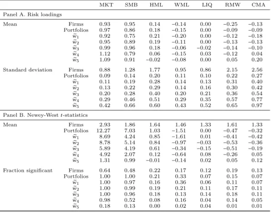
risk loadings that are statistically different from zero. To conserve space, we only present the results of risk loadings on all risk factors of the Fama and French (2015) five-factor model, and the momentum and liquidity factors of the Carhart (1997) four-factor model augmented with the liquidity four-factor of Pastor and Stambaugh (2003).
We find that it is often hard to obtain risk loadings that are statistically signif-icant. Table 2.5 shows that a substantial fraction of the risk loading estimates are
insignificant when individual firms are used as test assets. Only64%and48%of the
risk loading estimates are significant for the market and size factor, respectively, and most of the risk loadings corresponding to the other factors are insignificant. We attempt to alleviate the problem of using insignificant risk loadings by using random portfolios, which allow us to estimate risk loadings that are more precise as idiosyn-cratic risk is reduced through diversification. In line with this reasoning, our results
Table 2.5. Raw and Horizon-Specific Risk Loadings
This table presents risk loadings of raw and decomposed excess returns on 1,000 random portfolios. Results are presented for all the risk factors of the Fama and French (2015) five-factor model, and the momentum and liquidity factors of the Carhart (1997) four-factor model augmented with the liquidity factor of Pastor and Stambaugh (2003). The factors used are the market (MKT), size (SMB), value (HML), momentum (WML), liquidity (LIQ), profitability (RMW), and investment (CMA) factors. The results are for the maximum overlap discrete wavelet transform (MODWT) based on the least asymmetric Daubechies (1992) wavelet filter with eight lags (LA8). We exclude7× (2j−1)observations at the beginning of the resulting
time series to remove any effect of boundary conditions. In total we extract five components. We then estimate full sample risk loadings on a horizon-by-horizon basis. The presented risk loadings correspond to non-decomposed (Firms and Portfolios) and decomposed (we1towe5) excess returns and risk factors. In
Panel A, we present the mean and cross-sectional standard deviation of the estimated risk loadings, and in Panel B we present the mean Newey and West (1987)t-statistics and the fraction of the risk loading estimates that are statistically significant at the5%level. The sample period is from January 1968 to December 2015. We present average results based on 100 independent simulation runs.
MKT SMB HML WML LIQ RMW CMA Panel A. Risk loadings
Mean Firms 0.93 0.95 0.14 −0.14 0.00 −0.25 −0.13 Portfolios 0.97 0.86 0.18 −0.15 0.00 −0.09 −0.09 e w1 0.92 0.75 0.21 −0.20 0.00 −0.12 −0.18 e w2 0.95 0.89 0.19 −0.11 0.00 −0.13 −0.13 e w3 0.99 0.96 0.18 −0.06 −0.02 −0.14 −0.10 e w4 1.12 0.79 0.06 −0.15 0.03 −0.12 0.04 e w5 1.09 0.91 −0.02 −0.08 0.00 0.05 0.20 Standard deviation Firms 0.88 1.28 1.77 0.95 0.86 2.15 2.56
Portfolios 0.09 0.14 0.20 0.11 0.10 0.22 0.27 e w1 0.11 0.19 0.28 0.14 0.13 0.31 0.40 e w2 0.13 0.22 0.29 0.14 0.16 0.30 0.42 e w3 0.20 0.28 0.40 0.20 0.21 0.36 0.54 e w4 0.29 0.46 0.51 0.29 0.35 0.57 0.77 e w5 0.42 0.66 0.60 0.43 0.52 0.65 0.97 Panel B. Newey-Westt-statistics
Mean Firms 2.93 1.86 1.64 1.46 1.33 1.61 1.33 Portfolios 12.27 7.03 1.03 −1.51 0.00 −0.47 −0.32 e w1 8.69 4.24 0.85 −1.61 0.01 −0.41 −0.42 e w2 8.78 5.14 0.84 −0.97 −0.03 −0.53 −0.36 e w3 5.89 4.19 0.61 −0.34 −0.15 −0.51 −0.19 e w4 4.92 2.07 0.12 −0.64 0.08 −0.26 0.05 e w5 1.31 0.99 −0.01 −0.14 0.02 0.05 0.12 Fraction significant Firms 0.64 0.48 0.22 0.17 0.12 0.19 0.13
Portfolios 1.00 1.00 0.21 0.33 0.07 0.15 0.07 e w1 1.00 0.97 0.16 0.36 0.06 0.11 0.07 e w2 1.00 0.99 0.19 0.21 0.11 0.17 0.11 e w3 1.00 0.96 0.18 0.13 0.14 0.18 0.11 e w4 0.98 0.52 0.08 0.16 0.04 0.14 0.05 e w5 0.18 0.13 0.00 0.02 0.04 0.01 0.01