Monetary and macroprudential policies

Temi di Discussione

(Working Papers)

Monetary and macroprudential policies

by Paolo Angelini, Stefano Neri and Fabio Panetta

801

ch 20

Temi di discussione

(Working papers)

Monetary and macroprudential policies

by Paolo Angelini, Stefano Neri and Fabio Panetta

The purpose of the Temi di discussione series is to promote the circulation of working

papers prepared within the Bank of Italy or presented in Bank seminars by outside economists with the aim of stimulating comments and suggestions.

The views expressed in the articles are those of the authors and do not involve the responsibility of the Bank.

Editorial Board: Marcello Pericoli, Silvia Magri, Luisa Carpinelli, Emanuela Ciapanna, Daniela Marconi, Andrea Neri, Marzia Romanelli, Concetta Rondinelli, Tiziano Ropele, Andrea Silvestrini.

MONETARY AND MACROPRUDENTIAL POLICIES

by Paolo Angelini*, Stefano Neri* and Fabio Panetta* Abstract

We use a dynamic general equilibrium model featuring a banking sector to assess the interaction between macroprudential policy and monetary policy. We find that in “normal” times (when the economic cycle is driven by supply shocks) macroprudential policy generates only modest benefits for macroeconomic stability over a “monetary-policy-only” world. And lack of cooperation between the macroprudential authority and the central bank may even result in conflicting policies, hence suboptimal results. The benefits of introducing macroprudential policy tend to be sizeable when financial or housing market shocks, which affect the supply of loans, are important drivers of economic dynamics. In these cases a cooperative central bank will “lend a hand” to the macroprudential authority, working for broader objectives than just price stability in order to improve overall economic stability.

JEL Classification: E44, E58, E61

Keywords: macroprudential policy, monetary policy, capital requirements.

Contents

1. Introduction... 5

2. Modelling macroprudential policies ... 9

2.1 Current modelling approaches to macroprudential policy ... 9

2.2 The key mechanisms in our model ... 11

3. Modelling monetary and macroprudential policies ... 14

3.1 Monetary policy... 14

3.2 Macroprudential policy: instruments... 15

3.3 Macroprudential policy: objectives ... 17

4. The interaction between macroprudential and monetary policies... 18

4.1 The setup of the exercise ... 18

4.2 Results with a technology shock ... 20

4.3 Results with a financial shock ... 22

4.4 An alternative macroprudential policy instrument: the loan-to-value ratio... 24

5. Robustness checks ... 25

6. Conclusions... 28

Tables and figures... 31

References ... 37

_______________________________________

1 Introduction1

The debate on macroprudential policies ignited by the financial crisis is in full swing. Essentially, it turns on the thesis that so far policymakers in different spheres – mainly financial supervisors, but also monetary policymakers and accounting standard-setters – have overlooked systemic risk, or at least not taken it properly into account. In the run-up to the crisis it was not clear who should be concerned with systemic risk. Micro-prudential supervisors typically focus on single institutions and are accordingly liable to neglect risks outside their purview – risks that may be negligible for the

individual institution but may nevertheless add up in the aggregate.2 Central banks

concentrate on price stability and may not be sufficiently concerned with financial stability. Meanwhile, the various financial sectors are often under the jurisdiction of different authorities, greatly complicating thorough analysis, let alone action, on systemic risk. These considerations, which loom large in the regulatory agenda, have led the major countries to establish new institutions, or strengthen existing ones, with a mandate for financial stability.3

Certainly, a primary purpose of macroprudential policies must be to limit the accumulation of financial risks, in order to reduce the probability and mitigate the impact

of a financial crash.4 Its pursuit will likely require the macroprudential authority to adjust

1

An earlier version of this paper was presented at the CEPR – European Banking Center conference “Procyclicality and financial regulation”, University of Tilburg, Tilburg, 11-12 March 2010, as “Macroeconomic Stabilization Policies: Grafting Macroprudential Tools in a Macroeconomic Framework”. We benefited from comments by Javier Bianchi, Martina Cecioni, Martin Eichenbaum, Luca Guerrieri, Matteo Iacoviello, Jinill Kim, Robert Kollman, Caterina Mendicino, Alessandro Notarpietro, Simon Potter, Pau Rabanal, Sergio Santoro, Luca Sessa and Skander Van den Heuvel. We thank participants at seminars at the European Central Bank, the Norges Bank, the International Monetary Fund and the Board of Governors of the Federal Reserve as well as participants at the above mentioned CEPR/EBC conference, the Hong Kong Institute for Monetary Research/BIS conference “Financial Stability: Towards a Macroprudential Approach”, 5-7 July 2010, and the EIEF-Banca d’Italia-Banque de France conference “The future of monetary policy”, 30 September - 1 October 2010. The views expressed in the paper do not necessarily reflect those of the Bank of Italy. Corresponding author: Stefano Neri, e-mail: [email protected]

2

See Brunnermeier et al., (2009).

3

Newly established macroprudential institutions are the European Systemic Risk Board (ESRB) in the European Union and the Financial Stability Oversight Council (FSOC) in the United States. In the United Kingdom the 2009 Banking Act gives the Bank of England broad powers in this field.

4

A second key purpose is to strengthen the resilience of the financial sector. This can be achieved by a variety of tools: higher capital requirements, new liquidity buffers (Committee of European Banking Supervisors, 2009), policies to address the “too-big-to-fail” problem, regulation of derivatives markets (Financial Stability Board, 2009). The adjustment of these tools would likely be infrequent or even one-off. Economists quite commonly

its policy tools dynamically, to counter the build-up of risks during upswings and attenuate credit contraction and excessive risk-aversion in downturns.

In this paper we study the effectiveness and consequences of these macroprudential policies and their interaction with monetary policy. Our motivation is fourfold. First, countercyclical macroprudential policy is linked to other policies that moderate cyclical fluctuations – above all monetary policy, which bears on such macroprudential variables as asset prices and credit. And as macroprudential policy has direct or indirect effects on these variables it is likely to influence the transmission mechanism of monetary policy. Yet the interaction between the two has received surprisingly little attention.

Second, there is a relatively well-defined set of proposals for the instruments of macroprudential policy. Countercyclical capital requirements and loan-to-value (LTV) ratios are at the centre of the policy debate. Some countries have already started using them, and the new macroprudential authorities established in the main world regions may

well follow suit soon.5 In addition, the newly approved Basel III reform package

envisions a countercyclical capital buffer. So it is important to assess the performance of these instruments in a macro context.

Third, the institutional framework for the relationship between the macroprudential authority and the central bank differs from country to country. At one extreme, the Bank of England has been assigned full responsibility for macroprudential policy. In the European Union, central banks have a prominent role in the ESRB, although other institutions (e.g. financial supervisors) are also represented. The United States is close to the opposite extreme: the Federal Reserve participates in the FSOC with nine other members, but has no privileged role save that warranted by its superior skills in macroeconomic and financial analysis. Each of these institutional setups has pros and cons. Having two independent authorities may enhance accountability and reinforce the commitment needed to achieve objectives, but with a risk of coordination failures that may well yield suboptimal results.

Finally, analysis of the proposals on macroprudential policies has generally lacked the sort of consistent framework that would allow a structured approach. As a result, the distinguish between these two goals, which are not mutually exclusive. See Borio (2003), (2010), Bank of England (2009), Committee on the Global Financial System (2010).

5

Korea introduced caps on LTV ratios in 2002, adjusting them periodically to offset the build-up of pressures in the housing market. The Hong Kong SAR tightened mortgage LTV ratios in August 2010. China and Singapore also recently announced higher down-payment requirements for house purchases.

process of institutional reform is well ahead of its theoretical and practical underpinning, and faces important challenges. At best, the new macroprudential authorities will have to “invent” ways to perform their functions. At worst, they may fail to achieve their objectives.

This paper presents a framework within which to analyse the impact of macroprudential policy and its interaction with monetary policy on macroeconomic performance and stability. We introduce a formal definition of macroprudential policy objectives and instruments in a macroeconomic model. This presents several challenges. First, modelling macroprudential policy – objectives and instruments – is largely uncharted territory. While a new strand of literature (surveyed below) is developing rapidly, the financial sector has been relatively neglected in macroeconomics until recently and is still largely ignored in discussions of policies’ implications for financial stability. Second, like most macroeconomic models ours does not explicitly include the distortion that macroprudential policy should address, namely systemic risk. This partly

reflects the elusive nature of systemic risk, which impedes fully rigorous modelling.6

Since these difficulties put a rigorous normative approach beyond reach for now, we adopt a positive approach. That is, we take the presence of macroprudential regulation for granted. We do not analyse its rationale or microeconomic determinants but only study its effect on the economy and its interaction with monetary policy. To model the operational objective and tools of the macroprudential authority, we draw on policymakers’ stated goals and the actions they have taken. As to the objective, there is broad consensus on avoiding “excessive” lending to the private sector and containing the cyclical fluctuations of the economy. So we assume that the macroprudential authority minimizes a loss function whose arguments are the variances of the loans-to-output ratio and of output. We discuss these choices and assess the robustness of our results to alternative objectives. As

to instruments, we take countercyclical capital requirements and LTV ratios.7 Our

modelling of monetary policy is standard: the central bank sets the parameters of a simple Taylor rule to minimize the variance of inflation and output. Overall, we believe that our

6

Systemic risk can arise in different ways with respect to market participants (a bank run or the default of an investment firm), markets (stock market crashes or currency crises) and geographical areas (domestic vs. international crises).

7

Clearly, other instruments could be examined, depending on the nature of the risk considered. A systemic shock to funding and market liquidity would require measures targeted specifically to illiquidity problems (see for instance Perotti and Suarez, 2010).

approach is a useful starting point for addressing the formidable conceptual and practical problems of modelling countercyclical macroprudential policy.

We posit two cases of interaction between macroprudential and monetary policy. In the “cooperative” case, the two authorities jointly and simultaneously implement their policy rules in order to minimize a common objective (loss) function. In the “non-cooperative” case each authority minimizes its own objective function, taking the other’s policy rule as given.

We use the dynamic stochastic general equilibrium (DSGE) model developed by

Gerali et al. (2010), which has some useful features for our purpose. For one, it is

estimated, which makes it particularly appropriate for a positive analysis such as ours. More importantly, it incorporates a banking sector and its meaningful interaction with the

real economy, which the DSGE models of the previous generation did not.8 While simple

enough to allow us to trace the source of the main effects, our banking sector is also realistic enough to allow the proper modelling of our two candidate macroprudential policy instruments, which affect real and financial variables through channels independent from monetary policy. In particular, the supply of credit to the real economy is constrained by the availability of bank capital (as in the Basel regulation), which can only be accumulated gradually through retained earnings. This friction makes the economy vulnerable to a shock to bank capital and gives a potentially powerful role to macroprudential policy. In the event of a negative shock to bank capital, lowering the requirement could avert deleveraging and its repercussions on economic growth. Notice that this intervention would be genuinely macroprudential in nature, in that in these circumstances a microprudential regulator would want to increase capital requirements.

Our results suggest that macroprudential policy can improve macroeconomic stability, but important qualifications are needed. In “normal” times – when the cycle is mainly driven by supply shocks – macroprudential policy yields negligible additional benefits over a “monetary-policy-only” world, even if the two authorities cooperate; and non-cooperation may even produce excessive volatility of the policy tools (interest rates for the central bank, capital requirements for the macroprudential authority). This is because macroprudential policy and monetary policy act on closely related variables

8

The financial accelerator mechanism of Bernanke et al. (1999) has only recently been re-considered in standard medium-scale DSGE models (see for example Gilchrist et al., 2009).

(interest rates, credit supply, etc.) but have different objectives, so that at times they may push in different directions.

The benefits of introducing macroprudential policy become sizeable when economic fluctuations are driven by financial or housing market shocks, which affect the supply of loans, and are greater still when the central bank and the macroprudential authority cooperate closely. In this case the former “lends a hand” to the latter, working for objectives beyond mere price stability in order to enhance the overall stability of the economy.

All in all, our results suggest that the benefits of macroprudential policy depend crucially on the source and magnitude of the shocks and on the degree of coordination with monetary policy. If mismanaged, macroprudential policy could generate undesired variability in economic variables such as interest rates and capital requirements without much improvement in other dimensions.

The paper is organized as follows. Section 2 reviews the recent literature on macroprudential policy modelling and describes our model. In particular, section 2.2 specifies the channels through which monetary and macroprudential policies independently affect the economy. Section 3 lays out the interaction between the two authorities, with a detailed discussion of the macroprudential objective function. Section 4 gives the main results, Section 5 offers a robustness analysis, and Section 6 concludes.

2 Modelling macroprudential policies

2.1 Current modelling approaches to macroprudential policy

The ideal framework within which to study macroprudential policy should be simple enough to allow a proper understanding of the underlying mechanisms but also realistic enough to offer guidance to policymakers in this new environment. That is, it should allow macroprudential policy and monetary policy to coexist usefully (hard to do

in a simple framework).9 Another important requisite for such a framework should be

allowance for the particular distortion that macroprudential policy is supposed to address – systemic risk.

9

For instance, in a standard AS-AD New Keynesian model, the two policies would be linearly dependent, insofar as both ultimately influence the only control available to the policymaker, the interest rate – either via open market operations or via changes in the capital requirement.

These features are rarely combined in a single model. To our knowledge, none of the existing analytical frameworks features full-fledged modelling of systemic risk, although several recent contributions come close. Bianchi (2009), Bianchi and Mendoza (2010), Mendoza (2010), and Jeanne and Korinek (2010), modifying the framework pioneered by Kiyotaki and Moore (1997), show that when access to credit is subject to an occasionally binding collateral constraint, a credit externality arises, driving a wedge between the competitive and the planner equilibria. The externality induces households to overborrow, as they fail to internalize the effect of their own actions on the price of the collateral. But it is not clear how robust this externality is. Depending on certain features and parameterizations, the model can display not only overborrowing but also

underborrowing (Benigno et al., 2010), which may even predominate (Benigno et al.,

2011).10 Brunnermeier and Sannikov (2011) study a continuous-time, global

(non-linearised) model in which certain agents (“experts”) have superior skills in selecting profitable projects but limited net worth. In normal times the economy is in a steady state with low volatility, but it occasionally lapses into a regime with high volatility induced by strong negative feedback from large losses by the “experts”. At the heart of the loop there lies an externality, in that individually market participants take prices as given, but collectively they affect them. A common problem with these models is that in order to overcome technical and computational complexities they are extremely simplified. Often they have an insufficient level of detail in treating the financial sector or monetary policy, or both, and are accordingly unsuitable for our purposes.

Several recent papers have analysed issues of financial stability in more standard macroeconomic models. Woodford (2010) and Cúrdia and Woodford (2010), proxying financial instability by an exogenous process for the spread between loan and deposit rates, show that a Taylor-type monetary policy rule that also includes a forward-looking indicator of financial distress based on this spread is welfare-improving. But systemic risk is not modelled. Another strand in the literature uses models with a banking sector and bank capital. The paper most closely related to ours is Bean et al. (2010), presenting a modified version of Gertler and Karadi (2009) to study the interaction between monetary and macroprudential policy. However, they model macroprudential policy as a levy on (or subsidy to) banks that directly affects capital, whereas we model countercyclical capital buffers and loan-to-value ratios explicitly, which brings the analysis closer to the current

10

Bianchi and Mendoza (2010) themselves find that overborrowing arises in the competitive equilibrium for reasonable values of the key parameters, but not for all values.

policy debate. In Angeloni and Faia (2009) the banking system is subject to the risk of runs, and monetary policy reacts not only to inflation and output but also to asset prices or

leverage. Kannan et al. (2009) use a DSGE model with housing and find that a

macroprudential tool to attenuate the credit cycle can help monetary policy in stabilizing the economy. Covas and Fujita (2010) examine the effects of capital requirements on the business cycle in a model with agency problems à la Holmstrom and Tirole (1998). N’Dyaie (2009) finds that countercyclical capital rules enable the monetary authorities to

achieve their output and inflation targets with smaller changes in interest rates. Catte et al.

(2010), positing that the macroprudential authority can directly affect mortgage spreads, show that a tightening through this instrument would have curbed the US house price boom between 2003 and 2006 with modest repercussions on the other variables. A common finding of these papers is that a macroprudential instrument to moderate the credit cycle could potentially reduce output fluctuations. Ordinarily, however, they do not consider strategic interactions between macroprudential and monetary policy.

2.2 The key mechanisms in our model

In this paper we take the DSGE model developed in Gerali et al. (2010) as a suitable

middle ground in the trade-off between simplicity and realism. To a model with credit frictions and borrowing constraints, as in Iacoviello (2005), and a set of real and nominal

frictions, as in Christiano et al. (2005) or Smets and Wouters (2003), Gerali et al. (2010)

add a stylized banking sector. The economy is populated by entrepreneurs, heterogeneous households and monopolistically competitive banks. Patient households (the savers) deposit their savings in the banks. Impatient households and firms borrow, subject to a

binding collateral constraint.11 Firms produce consumer and investment goods using

labour supplied by households and capital. Banks’ assets are loans to firms and households, their liabilities are deposits and capital.

Banks aim at keeping the capital-asset ratio close to an exogenous target level ν, which we interpret as a capital requirement imposed by the regulator, as in the Basel

Accords. We do not provide microfoundation requirements.12 This target incorporates

11

Technically, the two types of household differ in the discount factor they apply to the stream of future utility. This heterogeneity gives rise to borrowing and lending in equilibrium (see Gerali et al., 2010).

12

See e.g. Acharya et al. (2010) for a microfoundation of bank capital and a justification of regulatory minimum requirements. In their framework, the optimal capital structure balances the benefits of high leverage (ensuring adequate monitoring by creditors and shareholders, to limit rent-seeking by managers) against its drawbacks

(risk-into the model the basic accelerator mechanism described by Adrian and Shin (2008), which arguably played a major role in the financial crisis.13 The exogeneity of ν is an important feature of our model, discussed below.

In what follows we present the equations that are crucial for the interaction between monetary policy and our two macroprudential instruments; for a full description of the

analytical framework see Gerali et al. (2010).

We start with the equations for the analysis of countercyclical capital requirements.

Bank capital Kb,tis accumulated out of retained profits Πb:

(1) K_b,t =

(

)

where δb is a depreciation rate. By equation (1), banks can increase their capital only through retained earnings. This is another important feature of our model, to which we

return below. The interest rate on loans to credit-constrained households (H) and

entrepreneurs (E) is given by the following first-order condition:

(2) _{t t}Bi t t b t i B t i B t Adj L K R R , , ' , + ,            − + =µ φ ν , i=H, E

where µ_tB,iis a non-zero-mean exogenous shock, which can be interpreted as a

time-varying mark-up arising from banks’ monopolistic power; Rt is the monetary policy rate;

'

φ is the first-order derivative of a decreasing and convex function measuring the costs

incurred by the bank when the ratio of its capital to loans (L) deviates from the

requirement νt set by the macroprudential authority; and the term Adj captures the costs

for adjusting bank rates, accounting for their stickiness.14 Equation (2) can be interpreted

as a loan supply schedule. When loans increase, the capital-asset ratio falls below νt,

inducing the bank to raise the lending rate. This, in turn, reduces the demand for credit.

shifting to the detriment of debt-holders). Van Den Heuvel (2008) presents a microfoundation of capital in a general equilibrium model.

13

We distinguish between the capital-asset ratio and leverage, as we modify the adjustment cost function used in Gerali et al. (2010) to account for the risk-sensitive regulation of capital. We replace total loans Lt with the sum of

risk-weighted loans to firms LFt and to households L H

t. To account for cyclicality in risk weights, the empirical

specification assumes that they depend on the yearly output growth rate:

(

) (

)

w is the risk weight of agent type i and y is output. See Angelini et al. (2009) for a description of the estimation method.

14

This term comprises bank rates both lagged and expected one-period-ahead. It implies that the costs related to the bank’s capital position are transferred gradually to the lending rate.

The interest rate on deposits RD, the relevant rate for savers’ choices between consumption and savings, is given by:

(3) R_tD =µ_tDR_t +Adj_tB,D

where µ_tDis a non-zero-mean exogenous shock, which can be interpreted as a

time-varying mark-down on the policy rate, and the term Adj,similarly to Eq. (2),captures the

cost of adjusting the deposit rate.

Equations (2) and (3) help us see why in this model macroprudential and monetary

policies have independent roles. The monetary policy rate R_t has an immediate impact on

both the lending and deposit rates, but the macroprudential instrument νt has an immediate

impact only on the lending rate. Manoeuvring their instruments separately, the two policymakers can drive a wedge between the two rates and, ultimately, exert an

independent effect on the consumption choices of savers and borrowers.15

Next, we look at the main equations through which our second candidate macro-prudential instrument, the LTV ratio, affects the economy. The optimal consumption/saving choices of patient households and of credit-constrained households

are described by the following Euler equations (s and b superscripts stand for savers and

borrowers): (4) _      ₊ = + +1 1 t 1 1 E 1 t D t s t s s t R c c β π (5)

(

)

where βj are the discount factors, βs >βb; c is consumption; and π is inflation. The equations define the optimal consumption choices. For savers (equation 4) they depend on the current and expected real returns on deposits. For borrowers (equation 5) they depend

15

The Adj terms disappear if the assumption of sticky loan and deposit rates is dropped. Therefore, this assumption is not strictly necessary to study the role of capital requirements as a macroprudential policy tool. But the assumption of monopolistic competition is necessary, since without it steady-state bank capital will be zero. A spread between deposit and lending rates is also the channel through which financial factors enter the models in Cúrdia and Woodford (2010) and Woodford (2010). In their setup the spread depends on exogenous factors (such as bank intermediation costs) and debt. By contrast, in Bean et al. (2010) the spread is driven by monetary policy; macroprudential policy is directly modelled by a tax/injection of bank capital, which has a one-to-one effect on real investment by non-financial firms and is therefore very powerful.

on the current and expected real cost of bank loans R_tB,H, but also on λt, the Lagrange multiplier of the borrowing constraint:

(6) (1+R_tB,H)b_tH ≤mHE_t[q_th₊₁h_tπ_t+1]

where qthis the price of housing, ht the stock of existing homes,

H t

b _{the amount borrowed}

from banks, and m_tH the LTV ratio for mortgages.

Equations (4) through (6) show how macroprudential policy can influence the

economy independently of monetary policy. The monetary policy rate Rt affects both RD

and RB,H via equations (2)-(3), and hence the consumption and investment choices of

savers (via equation 4), and borrowers (via equation 5). In setting

m

policy affects the stringency of the borrowing constraint λt. This has no effect on equation

(4) but does affect equation (5). As the collateral constraint tightens and λt increases, borrowers’ ability to finance consumption and housing investment is reduced, so both

these types of spending fall.16 Note that in this case the independent role of

macroprudential policy stems from the presence of credit-constrained agents; in this

setup, if λt falls to zero monetary policy and macroprudential policy become linearly

dependent.

3 Modelling monetary and macroprudential policies

In this section we discuss the objectives and the instruments of the central bank and the macroprudential authority.

3.1 Monetary policy

We follow the standard practice and assume that the central bank instrument can be modelled via a Taylor rule with the following specification:

(7) R_t =

(

) (

)

[

(

)

(

)

]

16

A similar mechanism is at work in Cúrdia and Woodford (2010). The optimal choices of consumption and investment in physical capital by entrepreneurs are characterized by similar first-order conditions. Firms borrow from banks against the value of their physical capital.

where the parameter χ_π measures the response to deviations of inflation (π) from the

target, χ_y its response to the growth of output (y) and ρ_R the inertia in the adjustment of

the policy rate.

The central bank stabilizes inflation and output, selecting the parameters of the monetary policy rule (7) to minimize the following loss function:

(8) Lcb =σ_π2+k_y,cbσ_y2+k_rσ_∆2_r k_y ≥0,k_r ≥0,

where σ2 are the asymptotic (unconditional) variances of inflation and output growth and

of the changes in the policy instrument, i.e. the monetary policy rate. The weights ks

characterize the policymaker’s preferences over these variables. A positive kr is warranted

by the need to keep movements in the policy rate “reasonable”, since it is well known that if there is no cost for adjusting policy instruments, optimal policies will tend to generate excessive volatility in the policy rate. The loss function (8) could be obtained by taking a second-order approximation of the utility function of households and entrepreneurs, as in Woodford (2003) in the case of optimal monetary policy.

3.2 Macroprudential policy: instruments

We consider, one at a time, two macroprudential instruments: a capital requirement, and an LTV ratio. For capital requirements the rule is:

(9) ν_t =

(

) (

)

where the parameter ν measures the steady-state level of ν_t. Capital requirements are

adjusted according to the dynamics of a key macroeconomic variable Xt with a sensitivity

parameter χν. In the baseline simulations we set Xt equal to the growth of output. In this

case, a positive value for χν amounts to a countercyclical policy: capital requirements

increase in good times (banks must hold more capital for a given amount of loans) and decrease in recessions.17

We take capital requirements as our macroprudential instrument for two main reasons. First, based on past experience systemic crises inevitably affect bank capital and the supply of credit, either directly or indirectly. And – not surprisingly – bank capital has

17

Note that equation (9) affects the cyclical pattern of the variables but not their steady-state levels. This is because the model’s steady state is affected only by ν and not by the dynamics of the variables.

taken centre stage in the ongoing debate on regulatory reform. The capital rule (9) can be

viewed as an example of the countercyclical capital buffer introduced by Basel III.18

Restricting banks’ capital increases to retained earnings (equation (1)) carries two significant implications. First, it rules out all the other options for recapitalization discussed in the recent policy debate (contingent capital, public funds, etc.): interesting and important though they are, analysis of these options would require a far more complex model of banks’ sources of finance. Second, the lack of other sources of funds means that remedying a shortage of capital will take time; and, other things being equal, this makes macroprudential policy relatively powerful, which should be kept in mind in interpreting our results.

Our alternative macroprudential instrument is the LTV ratio, owing to its importance in the policy debate and the experience of the countries that already use it (South Korea, China, Singapore, Hong Kong). Moreover, the LTV ratio permits a robustness check on the results obtained with equation (9). We assume that the

macroprudential authority sets the LTV ratio mt for loans to households using a rule

similar to equation (9):

(10) m_t =

(

)

(

)

Our instruments do capture one essential aspect of macroprudential policy. As Hanson, Kashyap and Stein (2010) point out, when a microprudential regulator requires an undercapitalized bank to take prompt corrective action, it is indifferent whether the adjustment is made by increasing capital or decreasing assets, as long as the probability of default is lowered to an acceptable level. However, asset reduction by many banks at once would be likely to damage the economy, contracting aggregate credit supply: “...one can characterize the macroprudential approach to capital regulation as an effort to control the social costs associated with excessive balance-sheet shrinkage on the part of multiple financial institutions hit with a common shock” (Hanson, Kashyap and Stein, 2010). Our approach captures this essential feature of macroprudential policy: the danger of

18

One may wonder why banks do not follow a rule like (9) voluntarily. As we argued above, no rigorous answer is possible within our framework, since the externality that warrants macroprudential intervention is not present in our model. In practice, banks’ incentives to hold and manage capital may be reduced by the possibility of bailouts, or by managerial short-termism favoured by compensation schemes. Repullo and Suarez (2008) show that banks do have incentives to manage capital buffers countercyclically, but that these incentives, per se, are insufficient to eliminate the inherent pro-cyclicality of regulatory capital requirements.

excessive balance-sheet shrinkage may be averted if the macroprudential authority lowers the capital requirement.19

3.3 Macroprudential policy: objectives

Modelling the objectives of macroprudential policies is not easy, because systemic risk can come in various forms and environments and most macroeconomic models (including ours) have no specific proxy for it. Therefore, our specification of the authority’s loss function needs discussion. Our procedure could be described as a “revealed-preferences” approach: since the objectives of macroprudential policy are not clear yet, either in theory or in practice, we try to determine which goals macroprudential authorities are actually aiming for.

Several clues can be garnered from an influential policy paper by the Bank of England (2009), which defines one key source of systemic risk as the “strong collective tendency for financial firms, as well as companies and households, to overexpose themselves to risk in the upswing of a credit cycle, and to become overly risk-averse in a downswing” (p. 16). The paper says that macroprudential policy should ensure “the stable provision of financial intermediation services to the wider economy, [avoiding] the boom and bust cycle in the supply of credit …” (p. 9) and suggests framing the authority’s objectives in terms of “abnormal” credit expansion. This approach has both empirical and theoretical underpinnings. There is substantial evidence that abnormal credit expansions tend to lead to financial crises (Reinhart and Rogoff, 2008; Borio and Drehmann, 2009). As for theory, some of the works surveyed in section 2.1 suggest that the amplitude of fluctuations in credit cycles can be excessive.

On this basis we posit that macroprudential authorities take credit as an important indicator of financial stability and react to its “abnormal” behaviour. In our model the economy is more vulnerable to shocks when leverage (proxied by the loans-to-output

ratio) is greater.20 We therefore assume that one key argument of the loss function that the

authority seeks to minimize is the variance of the loans-to-output ratio, σ_l2_/y.

19

This may be difficult during a downturn, as the markets themselves may put pressure on banks to recapitalize (Diamond and Rajan, 2009). This concern could be addressed by raising the requirement in normal times so as to lend credibility to the reduction dictated by equation (9) in bad times.

20

The greater the leverage, the more consumption and investment respond to changes in the price of collateral (housing and capital) and lending rates (see Iacoviello, 2005).

A second policy reference, Committee on the Global Financial System (2010), calls for macroprudential policy to mitigate the “...risk of a disruption of financial services that .... has the potential to have serious negative consequences for the real economy”. Based on this indication, we assume that the authority is also interested in minimizing fluctuations in output.

Finally in our model the macroprudential authority, like the central bank, is concerned with the variability of the chosen policy instrument and needs to hold its movements within reasonable bounds. We accordingly assume that the authority minimizes the following loss function:

(11) Lmp =σ_l2_/y+k_y,mpσ_y2+k_νσ_∆2_ν

where mp stands for macroprudential and σ_∆2_ν is the volatility of the changes in the macroprudential instrument (banks’ capital requirements or LTV ratios).

Equation (11), in our view, captures some important features of the objectives that macroprudential authorities will likely set in practice. However, a case can also be made for different objective functions, so in section 5 we assess the sensitivity of our results to

alternative specifications of (11).21

4 The interaction between macroprudential and monetary policies

4.1 The setup of the exercise

In this section we study the interaction between monetary policy and macroprudential policy in two different cases. In the case of cooperation the policies are chosen jointly and optimally by a single policymaker with two instruments (the interest rate and the capital requirement), with the objective of stabilizing the variances of inflation, output, the loans-to-output ratio, and the changes in the instruments themselves. The resulting equilibrium can be taken as a situation in which the central bank is responsible for macroprudential policy or cooperates completely with the macroprudential

21

Forinstance, Bean et al. (2010) assume that the authority is interested in the volatility of output and of real capital. Also, one might argue that (11) should be cast solely in terms of output stabilization: why should the macroprudential authority care about the loans-to-output ratio, which is at best an indicator of financial instability that can lead to output disruption? We respond that in practice the new macroprudential authority is not going to be held accountable for any disturbance whatever to real economic activity, but only for disturbances that have a financial origin. Thus, its objective function will presumably include proxies for systemic risk in the financial system, such as the loans-to-output ratio.

authority. In formal terms, the values of the five policy parameters in (7) and (9) are optimal when they minimize the sum of the two loss functions (8) and (11):

(12) L=Lcb+Lmp =σ_π2 +σ_l2_/y+

(

)

where the superscripts cb and mp denote the central bank and the macroprudential

authority. The solution of this problem yields a tuple of parameters

) , ; , , (ρ_Rc* χ_πc* χc_y* ρ_νc* χ_νc* such that: ) , ; , , ( min arg ) , ; , , ( * * * * * ν ν π ν ν π χ ρ χ ρ χ χ ρ χ χ ρ R y c c c y c c R = L

subject to the constraint given by the model. The superscript c denotes the case of

cooperation.22

In the second case we assume that the monetary and the macroprudential policymakers do not cooperate: the former minimizes (8), taking the macroprudential policy rule (9) as given, while the latter minimizes (11), taking (7) as given. The solution of this interaction yields a tuple (ρ_Rn*,χ_πn*,χ_yn*;ρ_νn*,χ_νn*) such that:

) , ; , , ( min arg ) , , (ρ_Rn* χ_πn* χ_yn* = Lcb ρ_R χ_π χ_y ρ_νn* χ_νn* ) , ; , , ( min arg ) , (ρ_νn* χ_νn* = Lmp ρ_Rn* χ_πn* χ_yn* ρ_ν χ_ν

subject, again, to the constraint given by the model. The superscript n denotes the case of

non-cooperation: in practice, the policy chosen by each authority is optimal taking the other’s as given. In both cases households and firms are passive, taking policies as given. Our analysis resembles that of Petit (1989) and of Dixit and Lambertini (2003), in their studies of the interaction between monetary and fiscal policies.

We compare the outcomes of the two equilibria along different dimensions. In this

section the preference parameters are fixed as follows: ky,cb=0.5, kr=0.1 in (9), and

ky,mp=0.5, kν=0.1 in (11). The figures for the central bank preferences are broadly in line

with the values estimated in the literature (see, for example, Ozlale, 2003, and Ilbas,

22

A preliminary question is whether our instruments actually have the power to affect outcomes. For if their effect were negligible we would not be giving macroprudential policy a fair chance. To check this, we assume that the central bank has objective function (8) but can use two instruments, the policy rate and the capital requirement, according to (7) and (9); we then compare this case with the policy-rate-only case. Unreported results obtained for a technology shock show that adding the extra instrument can improve macroeconomic performance significantly.

2011) or used in the calibration of models (Ehrmann and Smets, 2003). In section 5, we check robustness with alternative parameterizations.

Preliminary attempts to minimize the joint loss (12) revealed that the results depended on initial conditions, which suggests that the function has several local minima. To make sure a global minimum was found, we randomly selected different tuples of

initial conditions for the parameters of the two policy rules (7) and (9).23 For

non-cooperation, we take as initial conditions the parameters of the two policy rules found in the case of cooperation.

4.2 Results with a technology shock

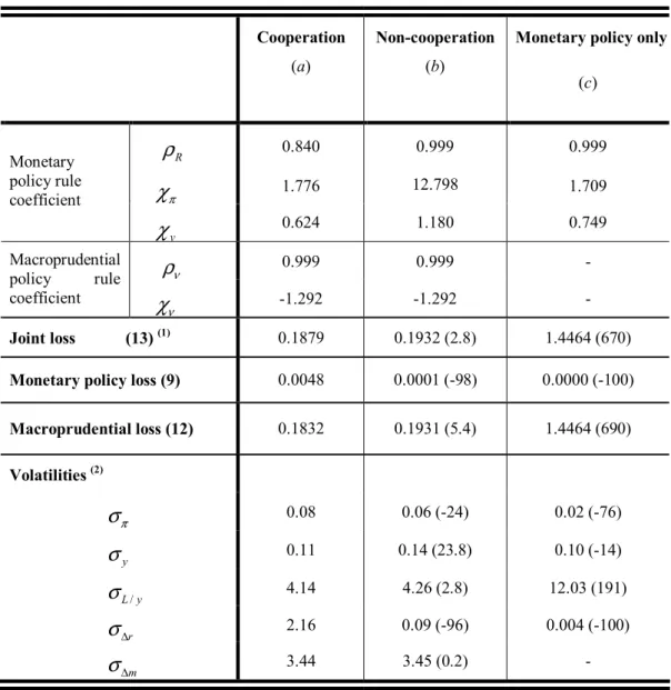
First we consider technology shocks, which are the main drivers of cyclical fluctuations in our model. The key features of the different outcomes are set out in Table 1. We begin with the case of policy cooperation (column (a)). The values for the monetary policy responses to inflation and output growth are, respectively, 1.77 and

0.92.24 The optimized macroprudential policy rule suggests that in response to positive

output growth capital requirements are tightened (the coefficient χν is 1.98).25

Under non-cooperation – column (b) – the strategies of the two policymakers are

quite different. Macroprudential policy becomes procyclical (χν turns negative), while

monetary policy is strongly countercyclical (χy increases to around 65). The joint loss,

computed as the sum of the two separate losses, is 4.1 percent worse than with cooperation. The central bank stands to benefit from cooperation (its loss function worsens by 8.7 percent under non-cooperation).

Looking within the loss functions in the two cases, the main difference is in the volatility of the policy instruments: the variability of the policy rate is 12 times greater under non-cooperation, that of capital requirements twice as great. This reflects the

23

The initial values for χR, χy and χν were drawn from uniform distributions. The ranges are, respectively, [1.7, 3.0],

[0.0, 1.0] and [-5.0, 5.0]. The initial values for ρR and ρν were fixed at 0.99 because they either converge to unit

values, as we show below, or yield local minima.

24

The optimized coefficients of the monetary rule suggest that strict inflation targeting is not optimal. This reflects the frictions present in the model. As is shown by Monacelli (2007), with financial frictions à la Kiyotaki and Moore (1997), monetary policy has to balance the incentive to undo the price rigidities against that to relax borrowing constraints by allowing for inflation variability. In our model strict inflation targeting would reduce the volatility of inflation but increase that of output and of the loans-to-output ratio.

25 _{Both policy rules are extremely inertial. The autoregressive parameters} ρ_{oftenhit the boundary (set at 0.999 to}

avoid numerical problems). This compares with a value of 0.77 in the monetary policy rule estimated in Gerali et al. (2010) and reflects the great persistency of the technology shock and its effects . If we repeat our exercise assuming less persistent shocks, the high persistence of the policy rules also tends to vanish.

central bank’s strong reaction to output growth and the procyclical behaviour of macroprudential policy and implies that the non-cooperative solution may give rise to substantial problems of coordination. The outcome is reminiscent of the finding of Dixit and Lambertini (2003) that a non-cooperative game between the monetary and fiscal authorities can result in low output and high inflation because fiscal policy is over-restrictive and monetary policy over-expansive.

Why does this conflict arise? Figure 1, showing the impulse responses of the key variables to a negative technology shock, can help us understand their dynamics in the two cases (we also report results for the case in which there is only monetary policy). First consider the case of cooperation. The combined reaction of the two authorities to the shock lowers capital requirements – allowing banks to reduce the capital/asset ratio by more than would have been possible otherwise, thus containing the rise in the loan rate – but produces almost no change in the monetary policy rate (balancing the contraction of output with an increase in inflation).

Next consider non-cooperation. Now the macroprudential authority, faced with an increase in the loans-to-output ratio – a signal of credit “overheating” – reacts by tightening capital requirements, potentially aggravating the fall in output. The central bank is therefore induced to ease aggressively. This, in turn, leads the macroprudential authority to tighten further, and so on. As a result of this interaction, in the non-cooperative case macroprudential policy increases capital requirements substantially in response to the rise in the loans-to-output ratio, in spite of the decline in output. Monetary policy offsets this by an equally sharp cut in interest rates.26 Clearly, this pattern is

suboptimal.27 As we shall see, better macroeconomic results are achieved in the

monetary-policy-only case – a world with no macroprudential policy.

The conflict stems from the coexistence of two independent authorities that work on closely related variables (interest rates and credit supply) but with different objectives. The macroprudential authority is interested in financial variables, the central bank only in output and inflation. Because the technology shock drives the loans-to-output ratio up and output down, without coordination the two policymakers may adopt conflicting policies

26

The dynamics of the loan rate is dominated by the reduction in the policy rate, which prevails over the increase in the cost of adjusting bank capital (induced by higher capital requirements and by the lower capital/asset ratio; see equation 2). Overall, however, the effects of the two different policy scenarios on output and inflation are barely distinguishable.

27

(the two policies remain compatible in the case of shocks that drive the two variables in

the same direction).28 Although the specification of (11) is ad hoc, our analysis

nevertheless captures a general result that can emerge whenever the objectives of the macroprudential and monetary authorities are not aligned.

The last column of Table 1 refers to the case in which macroprudential policy is absent and the central bank follows the Taylor rule (7) to minimize its loss function (8). By comparison with the cooperative equilibrium, the joint loss is practically unchanged, but the volatility of the interest rate declines substantially. Surprisingly, the variance of the loans-to-output ratio is significantly lower than in the previous two cases. These results apparently suggest that monetary policy alone can do a reasonably good job in attaining both monetary and macroprudential objectives. To put it another way, in this scenario macroprudential policy would appear to have little if any use. But the outcome is quite different in the case of a financial rather than a technology shock, as we discuss in section 4.3.

To sum up, under a technology shock the benefits of macroprudential policy are modest relative to the monetary-policy-only scenario. Indeed, lack of cooperation between the central bank and the macroprudential authority could even generate a conflict between the two policies, accentuating the variability of the policy instruments, as the macroprudential authority seeks to stabilize the loans-to-output ratio (an indicator of finance-driven instability), whereas the central bank cares only about output and inflation.

4.3 Results with a financial shock

We now replicate our analyses to examine the effect of a financial shock. Following

Gerali et al. (2010), we model the financial shock as an exogenous and unexpected

destruction of bank capital, affecting the real economy through its impact on the supply of

credit and on bank lending rates.29 The results are reported in Table 2.

28 _{Indeed, if the weight of the loans-to-output ratio in equation (12) is sufficiently small, the conflict tends to vanish.}

Unreported analyses show that the macroprudential tools may also move procyclically in the case of cooperation, but only for a narrow set of configurations of the preference weights (very little weight on output and very large weight on the loans-to-output ratio).

29

The financial shock is accompanied, in the exercise, by a shock to household preferences, in order to capture the decline in consumer confidence during the crisis; this does not affect the conclusions but makes our results more realistic and easier to interpret. The preference shock, as in Smets and Wouters (2003) is modelled as a shock to consumption within households’ utility function. In unreported simulations in which no allowance for the preference shock is made, the main results are unaltered.

Under cooperation, monetary policy responds aggressively to inflation and output growth, and the macroprudential policy rule also calls for a strong countercyclical

response to output (χν equals 9.6). Under non-cooperation macroprudential policy is

unchanged, but the monetary policy response to output is significantly weaker; the joint loss is 5.8 percent greater than with cooperation. Two key differences with respect to the technology shock emerge. First, there is no conflict between the two policies, since the financial shock drives output and the loans-to-output ratio in the same direction (although the central bank’s much more limited reaction to output indicates that a coordination problem may still be present). Second, with cooperation the central bank loses and the macroprudential authority gains. A possible interpretation is that with a financial shock the central bank may deviate from strict adherence to its own objective in order to “lend a hand” to maintain financial stability. This intuition is corroborated by the components of the loss functions: now the gains from cooperation stem from lower volatility in output, in the loans-to-output ratio and in the capital requirement, and are “paid for” by slightly greater variability of inflation and a more activist monetary policy (the volatility of the policy rate is greater with cooperation).

Column (c) of Table 2 compares cooperation with monetary-policy-only. Now, in contrast to the case of a technology shock, monetary policy alone is not enough to stabilize the economy. Instead, the availability of two policy instruments, if properly coordinated, generates sizeable gains for the stabilization of output and of the loans-to-output ratio.

Panel B of Figure 1, which reports the impulse responses to a financial shock, helps us understand the behaviour of the policymakers. With cooperation, the authorities react to the shortfall in bank capital by easing both macroprudential and monetary policy. Under non-cooperation, instead, the monetary policy reaction is practically negligible, inducing a stronger macroprudential response; the shock has a greater impact on output and the loans-to-output ratio than with cooperation. In the monetary-policy-only scenario the impact is greater still, reflecting the sharper rise in the lending rate and contraction in loans.

To assess the role of macroprudential policy when the economy is highly sensitive to shocks to banks’ capital, we replicate our exercises, increasing the values for kb in equation (2), the parameter that measures the cost of deviating from the regulatory capital

recapitalization is very costly, owing, say, to an underdeveloped capital market, or to financial stress (when it is obviously very expensive to raise capital). Three main results

emerge. First, the gains from macroprudential policy are increasing with kb. When we set

kb at 5 times the baseline value estimated in Gerali et al. (2010), which is equal to 11.0,

with cooperation the overall loss is 40 percent less than in the monetary-policy-only case. Second, the gains derive from a large reduction in the volatility of output and of the loans-to-output ratio (which are both 45 to 55 percent lower than with only monetary policy), partly offset by a 20-percent rise in the volatility percent of inflation; these results reflect the fact that when macroprudential policy is introduced and the policymakers cooperate, the central bank internalizes objectives related to financial stability, partly deviating from its own loss function. Third, the difference between cooperative and non-cooperative scenarios – i.e. the gain from cooperation – increases substantially.

We can now summarize the results for the financial shock scenario. First, the benefits of macroprudential policy over the monetary-policy-only scenario are substantial, and they are proportional to the cost borne by banks for deviating from the requirement. Second, the gains from cooperation between monetary and macroprudential policy are small in terms of the overall loss function; and they derive from the greater stability of the key macroeconomic variables. If financial shocks are important factors in economic dynamics, then cooperation helps stabilize output and the loans-to-output ratio. These benefits are “paid for” by activist monetary policy and greater variability of inflation. In practice, in the presence of financial shocks the central bank deviates from strict adherence to its objectives in order to “lend a hand” to maintain financial stability.

4.4 An alternative macroprudential policy instrument: the loan-to-value ratio

In this section we replicate our exercises, but taking as our macroprudential instrument the loan-to-value ratio (LTV), i.e. replacing (9) with (10). We assume that the

LTV is adjusted in response to house prices – i.e. Xt in equation (10) is the growth of real

house prices, whereas in (9) it is output growth – because this is the key causal variable for the dynamics of loans to households, and because it appears to correspond to the actual behaviour of policymakers.

In the technology shock scenario, the most important results (unreported) are the following. First, the macroprudential authority adjusts LTV counter-cyclically. Second, the benefits of macroprudential policy are negligible by comparison with the

monetary-policy-only scenario. Third, the benefits of cooperation, as gauged by the joint loss, are modest . Again, this result conceals strong heterogeneity in the function’s components. Specifically, the non-cooperation case shows slightly lower volatility of output and inflation, but much greater variability of the two policy instruments than under cooperation. In general, all the main results listed in section 4.2 survive the switch to LTV as an alternative policy instrument and the use of a different indicator variable for setting it.

We also considered a persistent shock to the demand for housing (and hence to

house prices),30 considering that modifying LTV is clearly the best way to address

overheating in the housing sector. The results are reported in Table 3. First, the central bank is better off in the case of non-cooperation (its loss function and the volatility of the policy rate are both much lower). Second, cooperation yields benefits in terms of lower variability of output and of the loans-to-output ratio, “paid for” by heightened volatility of inflation and of the policy rate. This result should read along the same lines as in section 4.3: given a disturbance (here, the housing demand shock), the central bank deviates from strict adherence to its objectives in order to “lend a hand” to macroprudential policy. Third, the benefits of macroprudential policy are substantial by comparison with the monetary-policy-only scenario. The improvement, which is due entirely to the loans-to-output ratio, comes at the expense of greater volatility of loans-to-output, inflation and the policy rate.

These findings are consistent with those of sections 4.2 and 4.3: macroprudential policy has little to contribute in normal times (when the economy is driven by supply shocks) but much to do in facing sectoral shocks to the financial sector or the housing market. In these cases, enhancing the policymakers’ arsenal with an instrument specifically targeted to the relevant sector generates substantial macroeconomic advantages.

5 Robustness checks

Alternative parameterizations of the loss functions (9) and (11). This robustness check is important, because the parameter values for our baseline results are not based on strong a

30

Housing demand shocks are modelled as in Gerali et al. (2010) and capture exogenous shifts in the preference for housing. These shocks yield a persistent increase in real house prices.

prioris. Here we repeat the exercises of section 4 under alternative choices for the

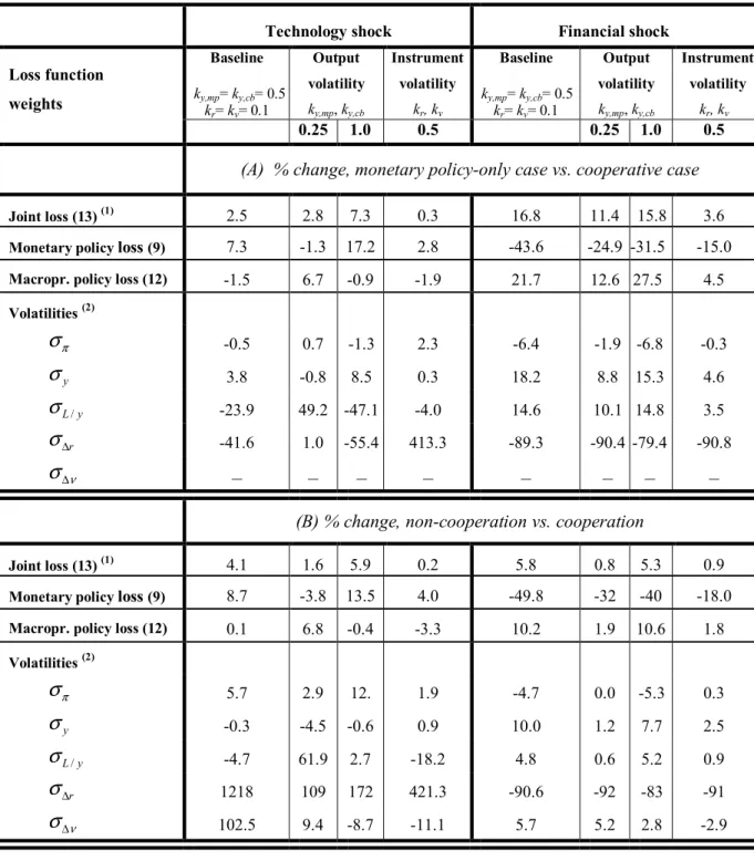
parameters ks of policymakers’ preferences for the various arguments. Table 4 reports the

main results for technology and financial shocks, giving the percentage differences in the objective functions and their components between the monetary-policy-only case and the case of cooperation (panel A); and between non-cooperation and cooperation (panel B). For ease of comparison with the baseline results, the first column of each panel reports the percentage differences taken from column (b) in Tables 1 and 2.

The check confirms most of our main results. In the case of technology shocks, no matter what weight is assigned to output volatility, macroprudential policy contributes very little to the joint stabilization of the objectives of the two policymakers (panel A). More precisely, when the importance of output is small for both policymakers (second column), the lack of macroprudential policy results in significantly greater volatility of the loans-to-output ratio but slightly lower variability of output. When output is an important policy consideration (third column), the opposite obtains. As for the benefits of cooperation, panel B confirms that they stem mainly from lower volatility of the instruments. As in the baseline case, this reflects countercyclical monetary and procyclical macroprudential policy.

The results obtained in the previous sections for financial shocks are also robust. In particular, in the monetary-policy-only case (right side of table 4, panel A) output and the loans-to-output ratio are consistently more volatile than under cooperation, for all our parameterizations. And the volatility of the policy rate is consistently lower, confirming that the central bank’s traditional loss function ignores financial stability. When both types of policy are in place, the failure to cooperate causes greater volatility of output and of the loans-to-output ratio and lower volatility of inflation and the policy interest rate (monetary policy does not “lend a hand” to preserve financial stability).

Alternative specifications of the loss function (11). A second key element underlying our results is the specification of the macroprudential policymaker’s preferences. Our choice of the arguments in (11) was determined by economic considerations and the simplified nature of our model, leaving only a narrow set of feasible and sensible alternative specifications. Given a crucial role of house prices in financial crises, one possible alternative specification would be to supplement (11) with a measure of house price volatility. Accordingly we simulated the model with technology shocks using a version of (11) augmented to include the variance of house prices (weighted at 0.5). The results are

qualitatively similar to those shown in section 4.2: the reduction in the overall loss produced by introducing macroprudential policy is small by comparison with the monetary-policy-only scenario. When both policies are in place, failure to cooperate creates the potential for conflict: macroprudential policy becomes procyclical while monetary policy is strongly countercyclical.

Alternative specifications for the macroprudential policy rule. Since the macroprudential authority is interested in the loans-to-output ratio, a natural alternative specification was to add that variable to the right-hand side of equation (10). The main results remain qualitatively unchanged. Under technology shocks, macroprudential policy contributes little to the stabilization of the two policymakers’ objectives. The benefits of cooperation tend to be smaller. Non-cooperation still produces coordination problems, resulting in great volatility of the policy rate, albeit less severe than in the baseline case. For financial shocks, the gains from macroprudential policy are greater than in the baseline case, as the macroprudential authority reduces the volatility of the loans-to-output ratio significantly. However, the benefit of cooperation relative to non-cooperation is more modest than in the baseline case.

Alternative shocks. We have also considered shocks other than technology, financial and housing. First, we replicate our exercises assuming a demand shock (modelled as shocks

to households’ preferences and to the efficiency of investment; see Gerali et al., 2010 for

more details). The comparison of cooperation with monetary-policy-only shows that once again the best outcome in terms of output and inflation is obtained in the latter case. This is not surprising, as demand shocks can be effectively offset by the central bank alone (they drive output and inflation in the same direction). Cooperation generates gains at the price of greater variability of the policy instruments, and in particular the policy rate.

Second, we considered a multi-shock scenario, factoring in all the shocks considered in Gerali et al. (2010). This exercise is warranted by the consideration that macroprudential policy, once in place, will be confronted with a set of shocks that are hard to disentangle. Indeed, this is arguably the most realistic scenario. Overall, the findings mirror those obtained assuming financial shock alone. The improvement brought about by macroprudential policy with respect to monetary-policy-only is substantial, regardless of the type of interaction between the two authorities. The gain reflects less volatility in output, inflation and the loans-to-output ratio, at the expense of greater variability in the policy rate.