NBER WORKING PAPER SERIES
HOUSING SUPPLY AND HOUSING BUBBLES Edward L. Glaeser
Joseph Gyourko Albert Saiz Working Paper 14193
http://www.nber.org/papers/w14193
NATIONAL BUREAU OF ECONOMIC RESEARCH 1050 Massachusetts Avenue
Cambridge, MA 02138 July 2008
We thank Jose Scheinkman, Andrei Shleifer, participants at the University of British Columbia's 2008 Summer Symposium on Urban Economics and Real Estate, the editors and referee for helpful comments on the paper. Naturally, we remain responsible for any errors. Glaeser thanks the Taubman Center for State and Local Government for financial support. Gyourko and Saiz thank the Research Sponsor Program of the Zell/Lurie Real Estate Center for the same. Finally, Andrew Moore provided excellent research support on the empirical work. Scott Kominers and Matt Resseger provided excellent research assistance on the theory. The views expressed herein are those of the author(s) and do not necessarily reflect the views of the National Bureau of Economic Research.
NBER working papers are circulated for discussion and comment purposes. They have not been peer-reviewed or been subject to the review by the NBER Board of Directors that accompanies official NBER publications.
© 2008 by Edward L. Glaeser, Joseph Gyourko, and Albert Saiz. All rights reserved. Short sections of text, not to exceed two paragraphs, may be quoted without explicit permission provided that full credit, including © notice, is given to the source.
Housing Supply and Housing Bubbles
Edward L. Glaeser, Joseph Gyourko, and Albert Saiz NBER Working Paper No. 14193
July 2008
JEL No. G12,R1,R31
ABSTRACT
Like many other assets, housing prices are quite volatile relative to observable changes in fundamentals. If we are going to understand boom-bust housing cycles, we must incorporate housing supply. In this paper, we present a simple model of housing bubbles that predicts that places with more elastic housing supply have fewer and shorter bubbles, with smaller price increases. However, the welfare consequences of bubbles may actually be higher in more elastic places because those places will overbuild more in response to a bubble. The data show that the price run-ups of the 1980s were almost exclusively experienced in cities where housing supply is more inelastic. More elastic places had slightly larger increases in building during that period. Over the past five years, a modest number of more elastic places also experienced large price booms, but as the model suggests, these booms seem to have been quite short. Prices are already moving back towards construction costs in those areas.
Edward L. Glaeser
Department of Economics 315A Littauer Center Harvard University Cambridge, MA 02138 and NBER eglaeser@harvard.edu Joseph Gyourko University of Pennsylvania Wharton School of Business 3620 Locust Walk 1480 Steinberg-Dietrich Hall Philadelphia, PA 19104-6302 and NBER gyourko@wharton.upenn.edu Albert Saiz University of Pennsylvania Wharton School of Business 3620 Locust Walk
1466 Steinberg-Dietrich Hall Philadelphia, PA 19104 saiz@wharton.upenn.edu
1
Introduction
In the 25 years since Shiller (1981) documented that swings in stock prices were
extremely high relative to changes in dividends, a growing body of papers has suggested that
asset price movements reflect irrational exuberance as well as fundamentals (DeLong et al.,
1990; Barberis et al., 2001). A running theme of these papers is that high transactions costs
and limits on short-selling make it more likely that prices will diverge from fundamentals. In
housing markets, transactions costs are higher and short-selling is more difficult than in almost
any other asset market (e.g., Linneman, 1986; Wallace and Meese, 1994; Rosenthal, 1989).
Thus, we should not be surprised that the predictability of housing price changes (Case and
Shiller, 1989) and seemingly large deviations between housing prices and fundamentals create
few opportunities for arbitrage.
The extraordinary nature of the recent boom in housing markets has piqued interest in
this issue, with some claiming there was a bubble (e.g., Shiller, 2005). While nonlinearities in
the discounting of rents could lead prices to respond sharply to changes in interest rates in
particular in certain markets (Himmelberg et al., 2005), it remains difficult to explain the large
changes in housing prices over time with changes in incomes, amenities or interest rates
(Glaeser and Gyourko, 2006). It certainly is hard to know whether house prices in 1996 were
too low or whether values in 2005 were too high, but it is harder still to explain the rapid rise
and fall of housing prices with a purely rational model.
However, the asset pricing literature long ago showed how difficult it is to confirm the
presence of a bubble (e.g., Flood and Hodrick, 1990). Our focus here is not on developing
such a test, but on examining the nature of bubbles, should they exist, in housing markets.
2
transfer large amounts of wealth between homeowners and buyers. Price volatility also
impacts the construction of new homes (Topel and Rosen, 1988), which involves the use of
real resources that could involve substantial welfare consequences. When housing prices
reflect fundamentals, those prices help migrants make appropriate decisions about where to
live. If prices, instead, reflect the frothiness of irrational exuberance, then those prices may
misdirect the migration decisions that collectively drive urban change.
Most asset bubbles also elicit a supply response, as was the case with the proliferation
of new internet firms in Silicon Valley in the late 1990s. Models of housing price volatility
that ignore supply miss a fundamental part of the housing market. Not only are changes in
housing supply among the more important real consequences of housing price changes, but
housing supply seems likely to help shape the course of any housing bubble. We show this is,
indeed, the case in Section II of this paper, where we develop a simple model to investigate
the interaction between housing bubbles and housing supply.
The model suggests that rational bubbles can exist when the supply of housing is fixed,
but not with elastic supply and a finite number of potential homebuyers. We model irrational,
exogenous bubbles as a temporary increase in optimism about future prices. Like any demand
shock, these bubbles have more of an effect on price and less of an effect on new construction
where housing supply is more inelastic. Even though elastic housing supply mutes the price
impacts of housing bubbles, the social welfare losses of housing bubbles may be higher in
more elastic areas, since there will be more overbuilding during the bubble.
We also endogenize asset bubbles by assuming that home buyers believe that future
price growth will resemble past price growth. Supply inelasticity then becomes a crucial
3
quickly comes on line as prices rise, which causes the bubble to quickly unravel. The model
predicts that building during a bubble causes post-bubble prices to drop below their pre-
bubble levels. The impact of housing supply elasticity on the size of the post-bubble drop is
ambiguous because the more elastic places have more construction during a bubble, but their
bubbles are shorter.
We then examine data on housing prices, new construction and supply elasticity during
periods of price booms and busts. While this empirical analysis is not a test for bubbles, much
of the evidence is consistent with the conclusions of our models. For readers who resolutely
do not believe in bubbles, the empirical results in the paper still provide information on the
nature of housing price volatility across markets with different supply conditions.
In performing the empirical analysis, we distinguish between areas with more or less
housing supply elasticity using a new geographical constraint measure developed by Saiz
(2008). We also investigate differences in price and quantity behavior between the most
recent boom and that which occurred in the 1980s.
During both the 1980s boom and the post-1996 boom, more inelastic places had much
larger increases in prices and much smaller increases in new construction. Indeed, during the
1980s, there basically was no housing price boom in the elastic areas of the country. Prices
stayed close to housing production costs. If anything, the gap in both price and quantity
growth between elastic and inelastic areas was even larger during the post-1996 boom than it
was during the 1980s. However, in the years since 1996, there were a number of highly elastic
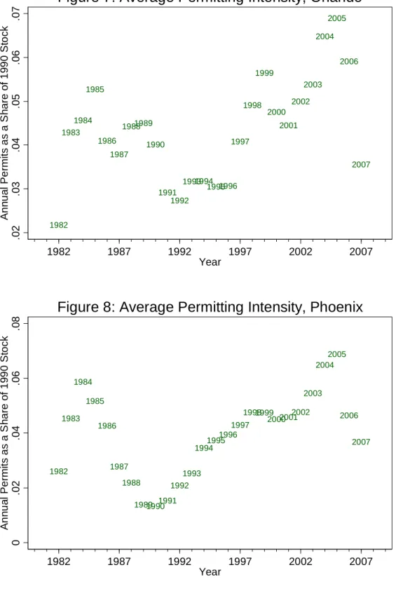
places (e.g., Orlando and Phoenix) that had temporary price explosions despite no visible
4
The fact that highly elastic places had price booms is one of the strange facts about the
recent price explosion. Our model does not suggest that bubbles are impossible in more
elastic areas, but it does imply that they will be quite short, and that is what the data indicate.
While the average boom in inelastic places lasted for more than four years, the average
duration of the boom in more elastic areas was 1.7 years.
Does the housing bust of 1989-1996 offer some guidance for the post-boom years that
are ahead of us? During that period, mean reversion was enormous. For every percentage
point of growth in a city’s housing prices between 1982 and 1989, prices declined by 0.33
percentage points between 1989 and 2006. The level of mean reversion was more severe in
more inelastic places, but on average, elasticity was uncorrelated with either price or quantity
changes during the bust.
Relatively elastic markets such as Orlando and Phoenix have not experienced sharp
increases in prices relative to construction costs in the past, so they have no history of
substantial mean reversion. Yet some insight into their future price paths might be provided
by the fact that for two decades leading up to 2002-2003, prices in their markets (and other
places with elastic supply sides) never varied more than ten to fifteen percent from what we
estimate to be minimum profitable production costs (MPPC), which is the sum of physical
production costs, land and land assembly costs, and a normal profit for the homebuilder.
Those three factors sum to well under $200,000 in these markets. If these markets return to
their historical norm of prices matching these costs, then they will experience further sharp
price declines. We now turn to the model that frames our empirical work.
5
A small, but growing, financial literature has examined the connection between
bubbles and asset supply by looking at lock-up provisions (Ofek and Richardson, 2003; Hong
et al., 2006). These provisions restrict the ability of asset owners to sell, and when they
expire, there can be a burst in the supply of shares on the market and a significant drop in
prices. In Hong, Scheinkman and Xiong (2006), the number of truly ebullient buyers is
limited, so the extra supply means that the marginal buyer is much more skeptical and prices
fall.1
Apart from this small but important literature, the bulk of the theoretical work on
bubbles written by financial and monetary economists has assumed that the supply of assets is
either fixed or determined by a monetary authority. While this assumption is appropriate for
some markets, it is not for housing markets, where new homes regularly are built in response
to rising prices. In this section, we incorporate housing supply into a simple model of
housing bubbles. In doing so, we treat irrational exuberance essentially as an exogenous
phenomenon, ignoring recent attempts to micro-found overoptimism (Barberis et al., 2001;
Hong et al., 2008). We focus on the extent to which supply mutes or exacerbates housing
bubbles and their welfare impacts.
We assume a continuous time model where a city’s home prices are determined by the
intersection of supply and demand. Demand comes from new homebuyers, whose willingness
to pay for housing is based on the utility gains from living in the city and expected housing
price appreciation. The supply of homes for sale includes new homes produced by developers
and old homes sold by existing homeowners. All homes are physically identical.
1 Shleifer’s (1986) work on whether the demand for stocks slopes down can be interpreted as a similar exercise
6
We differentiate between the stock of housing at time t, which is denotedH(t), and the
supply of homes for sale at that time period, which is denoted S(t). The supply of homes for
sale at time t combines the flow of new construction, denoted I(t), and older homes being put
on the market by their owners. The supply of new homes is determined by developers, and we
assume that the marginal cost of development equals c0 +c1I(t). This linear production cost reflects the possibility that there are scarce inputs into housing production, so that the cost of
production rises linearly with the amount of production.2 Ideally, we would model the decision of existing owners to sell as an optimization problem, but this would greatly
complicate the model. To simplify, we assume that each current homeowner receives a
Poisson-distributed shock with probabilityλ in each period that forces the homeowner to sell, leave the area and receive zero utility for the rest of time. Homeowners who do not receive
the shock do not put their homes on the market. While convenient, not allowing homeowners
to time their sale abstracts from potentially important aspects of housing bubbles.3 Even though each individual homeowner’s decision to sell is stochastic, we assume a continuum of
homeowners, so the number of existing homes for sale at time t is deterministic, proportional
to the existing stock of homes and equal toλH(t).
For the housing market to be in equilibrium, price (denotedP(t)) must equal
construction costs whenever there is new construction. The level of new homes for sale at
time t therefore equals the maximum of zero and
(
P(t)−c0)
/c1.Ours is an open city model in which demand comes from a steady flow of new buyers
who are interested in moving into the city. At every point in time, there is a distribution of
2 We could also assume that production costs rise with the stock of housing in the area, but this only adds
unnecessary complications.
3 However, Glaeser and Gyourko (2008) conclude the risk aversion limits the ability of consumers to arbitrage
7
risk-neutral buyers who are willing to purchase a home in the city if the expected utility gain
from living in the city plus the expected returns when they sell exceeds the price of the house.
Consumers have no option to delay purchase; they either buy at time t or live outside of the
city for eternity. We normalize the utility flow outside of the city to equal zero. Inside the
city, individual i receives a time-invariant flow of utility denominated in dollars equal to u(i),
until that person receives a shock that forces them to sell.
We further assume that, at all points of time, there is a distribution of u(i) among a
fixed number of potential buyers. Some people greatly benefit from living in the city, while
others gain less.4 Across buyers, the utility from living in the city, u(i), is distributed
uniformly with density 1 1
v on the interval [u,v0]. At any point in time, there is a marginal
buyer. Individuals whose utility flow from living in the city is greater than that of the
marginal buyer will purchase a home, while individuals whose utility flow from living in the
city is less than the marginal buyer will not. If the utility flow from the marginal buyer at time
t is denoted u*(t), then the number of buyers will equal 1 0 *( ) v t u v −
. This represents the level
of demand, D(t). Alternatively, we can invert the equation and write that the utility flow to
the marginal buyer equals v0 −v1D(t).
While the utility from living in the area is time invariant, buyers do recognize that at
each future date they will sell their homes with probabilityλand then receive the sales price of the house. Individuals who bought at time t understand that with probability 1−e−λjthey will
4 In the financial economics literature, it is less natural to assume that there is a heterogeneous demand for an
asset. Instead, heterogeneity is more likely to come from differences in beliefs among investers (Hong et al., 2006).
8
have sold their house and left the city by time t+j . This forward-looking aspect of the model
means that the current willingness-to-pay for housing will reflect expectations of future prices.
We assume that an individual making decisions at time t discounts future cash or utility
flows at time t+j with a standard discount factore−rj, where r is the interest rate. The expected
utility flow from someone who receives utility u(i) from living in the city is then given by
) ( ) ( ) ( ( )( ) t P dx x P e E r i u t x t x r t⎜⎝⎛ ⎟⎠⎞− + +
∫
∞ = − + − λ λλ , where Et
()
. reflects expectations as of time t. Ifthere is construction, the overall equilibrium in the housing market at time t satisfies:
(1) 0 1 ( ) E e ( )( )P(x)dx P(t) c0 c1(S(t) H(t)) r t D v v t x t x r t λ λ λ + ⎜⎝⎛ λ ⎟⎠⎞= = + − + −
∫
∞= − + − ,whereD(t)=S(t). Equation (1) represents a system of two equations (the consumer’s and developer’s indifference relations) and two unknowns (P(t) and D(t)). This system can be
solved as a function of the current stock of housing H(t) and expected future prices.
Rational, self-sustaining bubbles can satisfy the demand equation if there is no
building. For example, if D(t) equals a constant, D, and there is no construction, then the first
half of equation (1) will be satisfied at all t, if P(t) equals kert r D v v + − 1 0 , where k represents
an indeterminate constant of integration. The component rt
ke represents a “rational” bubble, where continuously rising prices justify continuously rising prices. When supply is fixed,
stochastic bubbles are also possible.5
While rational bubbles are compatible with a fixed housing supply, they cannot exist
with elastic housing supply and a finite number of potential homebuyers:
5There could be a bubble that ends with probabilityδ at each point in time, which survives with probability j e−δ for each period t+j, where prices equal ker t
r D v v0 1 ( +δ) + −
during the bubble and then fall to
r D v v0 − 1
after the bubble ends.
9
Proposition 1: If housing supply is elastic and the mass of potential buyers at each time t is finite, then there is no equilibrium where at any time t, P(t+ j)>c0 +ε , for all positive j and for any finite ε. (All proofs are in the appendix).
Perpetually rising prices means a perpetually rising housing supply, which eventually
means there are more homes being offered than there are potential customers in the market.
The result in the proposition hinges on our assumption of linear production costs, which
implies that there is no cap on the number of homes that could be produced. However, we do
not need such an elastic supply of housing to rule out rational bubbles. Rational bubbles
cannot exist if the supply of housing, given high enough prices, is greater than the maximum
possible number of buyers. Hence, we will turn our attention to irrational bubbles, but before
doing so, we discuss the equilibrium without irrationality.
In a perfectly rational world where supply rules out rational bubbles, the value of H(t)
determines whether the city is growing or stagnant. If
λ 1 0 0 ) ( v rc v t
H ≥ − , then prices will be
constant at r t H v v0 − 1λ ( )
, which is less than c0, and there will be no construction.
If λ 1 0 0 ) ( v rc v t
H < − , then construction will equal H t e j
v rc v γ λ γ − ⎟⎟ ⎠ ⎞ ⎜⎜ ⎝ ⎛ − − ) ( 1 0
0 at each date t+j, where
r v c r v r r .5 ) ( ) ( 25 . 1 1 1 2 − + + + + = λ λ λ
γ .6 Hereafter, we assume that
λ 1 0 0 ) ( v rc v t H < − so that the
6The total housing stock, H(t+j) will equal
⎟⎟ ⎠ ⎞ ⎜⎜ ⎝ ⎛ + − − + − − λ γ γ 1 0 0 0 ) 1 ( ) ( v rc v a e t H
e j j , and the amount of housing
on sale at any point in time is given by ⎟⎟
⎠ ⎞ ⎜⎜ ⎝ ⎛ − − + − − − + ( ) − ( ) 1 0 0 0 1 0 0 0 t H v rc v a e v rc v a j λ γ λ γ .
10
city is growing. At time t, the expected price at time t+j will equal
j e t H v rc v a c c γ λ γ − ⎟⎟ ⎠ ⎞ ⎜⎜ ⎝ ⎛ − − + + ( ) 1 0 0 0 1
0 , and we define this as PR,t(t+ j).
Irrational Bubbles
We now turn to less rational bubbles. We model such bubbles as a temporary burst of
irrational exuberance by buyers about future prices. We do not require that everyone share
this overoptimism, since there is no way of selling housing short in the model. Development
occurs instantaneously and reflects current, rather than future, prices so we can remain
agnostic about whether developers perceive the bubble in progress. The bubble acts much like
any other short-run increase to demand. Prices and construction levels temporarily rise and
then fall below equilibrium levels because of the extra housing built during the boom.
We begin by assuming that irrational bubbles represent a completely exogenous burst
of overoptimism about future prices that will last for a fixed period of time. Buyers do not
know that they are being influenced by a bubble. Equation (1) continues to hold, as long as
()
. tE is interpreted not as the rational expectation of future prices, but rather the
bubble-influenced expectation.
One method of introducing a bubble is to assume that buyers take today’s prices and
just have some optimistic rule of thumb about the future. We will investigate a model of this
form in the next section. In this section, we treat bubbles as an exogenous overestimate of
prices relative to the rational expectations equilibrium. Under some circumstances, this
exogenous overestimate might be justified by overoptimistic extrapolation, but that will not
11
If PR,t(t+ j) represents the correct expectation of future prices in the rational expectations equilibrium, then during the bubble people believe that future prices will equal
) (
, t j
PRt + plus some added quantity. Technically, we assume that during a bubble people overestimate the total value of
∫
∞= − + − t x t x r dx x P
e ( λ)( ) ( ) , relative to the rational expectations
equilibrium, by λ θ + r t) (
. For example, this would be satisfied if people believe future prices
will equal j t R t e r r j t P θ φ λ φ λ ) ( ) ( , + − + +
+ , but this is only one of many possibilities. The exact
nature of buyers’ beliefs is not critical for our purpose, as long as they believe that
∫
∞= − + − t x t x r dx x P e ( λ)( ) ( ) equals λ θ λ + +∫
∞= − + − r t dx x P e t x Rt t x r ( ) ) ( , ) )( ( .This error about future prices will then impact prices at time t, but the extent of this
influence depends on the elasticity of supply. If there were no supply response, then
over-optimism will raise prices by λ times λ θ + r t) (
. As mobility (λ) increases, the impact of incorrect future beliefs rises because more mobility causes people to care more about the
future. Allowing a construction response will mute the price impact of overoptimism because
added supply means that the marginal buyer has a lower utility benefit from living in the city.
In a growing city that experiences a bubble, prices at time t will equal the rational expectations
price, ⎟⎟ ⎠ ⎞ ⎜⎜ ⎝ ⎛ − − + + ( ) 1 0 0 0 1 0 H t v rc v a c c λ γ , plus 1 1 1 ) ( ) ( v c r t c + +λ θ λ
. The price impact of the bubble
increases with mobility and the inelasticity of supply (c1), and decreases with the
12
Our next two propositions consider the impact of an exogenous bubble whereθ(t)=θ
for the period t to t+k and then equals zero thereafter. Proposition 2 describes the general
impact of the bubble on prices, investment and the housing stock. Proposition 3 examines the
interaction between the bubble and housing supply elasticity. Recall that we assume
λ 1 0 0 ) ( v rc v t
H < − , so the city is growing:
Proposition 2: During the bubble, an increase in θ causes prices, investment and the housing stock to increase. The impact on prices and investment becomes weaker over the course of the bubble, but the impact on the housing stock increases over the course of the bubble. When the bubble is over, higher values of θ decrease housing prices and investment, and increase the housing stock.
During the period of the bubble (or any demand boost), there is a surge in prices and
new housing construction. Since the bubble’s magnitude is fixed during its duration, the price
and development impact of the bubble actually declines over time as new housing is built, but
this implication will disappear below when we assume that beliefs are fueled by the
experience of price growth.
When the bubble ends, housing prices fall below what they would have been if the
bubble had not happened. The price crash represents both the end of the overoptimism and the
extra supply that was built during the high price bubble period. The extra supply of housing
results in lower prices and construction levels ex post. Unsurprisingly, longer bubbles have a
larger impact. Our primary interest, however, is in the interaction between the bubble and
housing supply, which is the subject of Proposition 3:
Proposition 3: (a) During a bubble, higher values of c1-- a more inelastic housing supply--
will increase the impact of θ on prices. Higher values of c1will decrease the impact that θ
13
(b) After the bubble is over, higher values of c1 will reduce the adverse impact that
the bubble has on price levels when c1is sufficiently high, and will increase the impact that the
bubble has on prices when c1 is sufficiently low. If the bubble is sufficiently long, then
higher values of c1 increase the negative impact that the bubble has on price levels once it has
burst.
Part (a) of Proposition 3 details the impact that more inelastic housing supply
(reflected in higher values of c1) has on the bubble during its duration. When housing supply
is more inelastic, the bubble will have a larger impact on price and a smaller impact on the
housing stock. The impact of c1 on the flow of investment depends on the stage of the bubble.
Early in the bubble, places with more elastic housing supply will see more new construction in
response to the bubble. Over time, however, the housing investment response to the bubble
will actually be lower in places where supply is more elastic because there has already been so
much new building in those markets.
The interaction between an exogenous bubble and supply inelasticity is quite similar to
the connection between elasticity and any exogenous shift in demand. During the time the
bubble is raging, more inelastic places will have a larger shift in prices and will also
experience a sharper reduction in prices when the bubble ends. More elastic places will have a
larger increase in new construction, at least during the early stages of the bubble, and will
always experience a larger increase in total housing stock from the bubble.7
Part (b) of the proposition discusses the impact of housing elasticity on prices when the
bubble is over. The post-bubble impact on prices can either be larger or smaller in places with
more inelastic housing supply because there are two effects that go in opposite directions.
7 One of the counter-factual elements in this model is that prices and investment drop suddenly at the end of the
bubble rather than declining gradually, as they generally do in the real world. The price drop at the end of the bubble will be larger in more inelastic places with higher values ofc1. Higher values ofc1moderate the decline in new construction at the moment when the bubble ends.
14
First, places with more elastic housing build more homes in response to the bubble. These
extra homes act to reduce price levels when the bubble is over. Second, the impact of extra
homes on prices will be lower in places where housing supply is more elastic. Either effect
can dominate, so it is unclear whether the price hangover from a housing bubble is more
severe in places where supply is more or less elastic.
Just as more elastic housing supply can either increase or decrease the impact of the
bubble on ex post prices, more elastic housing supply can either increase or decrease the
welfare consequences of a bubble. Abstracting from the impacts that bubbles might have on
savings decisions or on risk averse consumers, the inefficiency of a housing bubble comes
from the misallocation of real resources—that is, the overbuilding of an area. This
overbuilding will be more severe in places where housing supply is more elastic.
We can calculate the expected welfare loss for a bubble that occurs only at period t, so
that buyers during that time period overestimate future prices, but no one after them makes
that same mistake. In that case, the number of people who buy housing at period t equals
1 1 1 0 0 0 ) ( ) ( ) ( ) ( v c r t t H v rc v a t H + + + ⎟⎟ ⎠ ⎞ ⎜⎜ ⎝ ⎛ − − + + λ λθ λ γ
λ , which equals the share of people who would
have bought housing absent the bubble plus
1 1 ) ( ) ( v c r t + +λ λθ
. The total welfare loss is found by
adding consumer welfare for the consumers who bought during that time period minus
development costs, or 1 1 2 2 ) ( ) ( v c r t + + − λ θ λ
. This is decreasing in c1. More inelastic markets will
have bigger price swings in response to a bubble, but the welfare losses will be smaller, since
15
The parallel of this in the real world is that if there is a housing bubble in a very
inelastic market such as greater Boston, prices may swing a lot, but there will be little change
in migration or construction patterns. If there is a housing bubble in a more elastic area such
as Phoenix and Orlando, then many thousands of extra homes will be built and many people
will make migration mistakes.
Self-Reinforcing Bubbles and Adaptive Expectations
The conclusion that greater resource misallocation results from overbuilding in more
elastic places assumes that the magnitude of the bubble is independent of housing elasticity.
However, if bubbles are endogenous and sustained by rising prices, then more inelastic places
might have bigger and longer bubbles, because rising demand is more likely to translate into
rising prices in those markets. To examine this possibility, we assume that bubbles take the
form of an irrational belief that prices will continue to rise at a fixed rate for all eternity.
We continue to work with our continuous time model, but we now assume that
individuals update their beliefs only at discrete intervals. For example, if the bubble begins at
time period t, then between period t and period t+1, individuals have exogenously come to the
view that future prices will increases perpetually so that buyers believe that P(t+ j)will equal j
t
P( )+ε • for all j. While this hybrid discrete-continuous time set-up is somewhat unusual, it is inspired by a financial econometrics literature examining settings where researchers only
observe a continuous time process at discrete intervals (Hansen and Scheinkman, 1995).
At time period t+1, individuals update their beliefs and base them on price growth
between period t and t+1. Between time periods t+1 and t+2, people extrapolate from price
16 ) 1 ( )) 1 ( ) 2 ( ( ) 1 (t+ + P t+ −P t+ • j−
P for all j. At every subsequent period t+x, where x is an
integer, updating again occurs. As long as prices continue to rise between period t+x and
t+x+1, buyers believe that future prices, P(t+ j), will equal ) ( ) 1 ( ) ( ( ) (t x P t x P t x j x
P + + + − + − • − .8 The future growth in price is assumed to equal the growth rate during the period between the last two integer time periods. We let g(t) denote
the expected future growth rate at time t.
As soon as price declines for one period, beliefs revert to rationality and the
equilibrium returns to the rational expectations equilibrium with, of course, an extra supply of
housing. If prices grow by less than they did the period before, prices will start to fall, and we
will refer to this as the end of the bubble.
We will normalize the date of the start of the bubble to be zero and assume that the city
has reached its long-run stable population level at that point, so that
λ 1 0 0 ) 0 ( v rc v H = − and 0 ) 0 ( c
P = . Because more housing will be built with the boom, if the irrational expectations disappear, the long-run steady state is that new construction will then end forever and H(t) will
remain at its highest level at the peak of the boom. Prices will then satisfy
r t H v v t
P( )= 0 − 1λ ( ) for the rest of time. We let HI(t)=H(t)−H(0) denote the incremental
housing built during the boom, so that
r t H v c t P( ) 1 I( ) 0 λ −
= after the bubble ends. New
housing built during the boom has a permanent, negative impact on prices after the boom is
over, since this city begins at steady-state population levels, but the impact of the amount of
housing built is independent of housing supply elasticity in the area.
8 See Mayer and Sinai (2007) for a recent examination of the possible role of adaptive expectations in the recent
17
The demand side of the model is captured by the equation:
(1’) ) ( ) ( ) ( )) ( ) ( ) ( ( ) ( ) ( 0 1 ( )( ) 0 1 λ λ λ λ λ + + − = ⎟ ⎠ ⎞ ⎜ ⎝ ⎛ + • − + + − =
∫
∞ = − + − r r t g r t D v v dj t x t g t P e E r t D v v t P t x t x r t ,which must hold throughout the bubble. The supply side continues to satisfy
) ( ) ( 1 0 c I t P t
c + = , which implies that
1 1 1 ( ) ) /( ) ( ) ( v rc t H v r t g t I I + − +
=λ λ λ . Including the supply
response into the pricing equation implies that ⎟
⎠ ⎞ ⎜ ⎝ ⎛ − + + + = ( ) ( ) ) ( 1 1 1 1 0 v H t r t g v rc c c t P I λ λ .
Unsurprisingly, supply mutes the price response to optimistic beliefs.
During the first period, individuals believe that g(t)=ε. In the second period, g(t) reflects the price growth during the first period. In the third period, g(t) reflects the price
growth during the second period. For the bubble to continue, not only must prices rises, but
they must rise at an increasing rate. Without ever-increasing optimism, new construction
would cause prices to fall. Yet, the ever-rising prices that are needed to fuel increasingly
optimistic beliefs are only possible if housing supply is sufficiently inelastic and if people are
sufficiently patient: Proposition 4: If r r − < 1 2
λ , then no bubble can persist beyond the first time period. If r r − > 1 2
λ , then at time one, there exists a c1, denoted c1*, where an initial bubble will persist if
and only if * 1 1 c c > . If r r − < 1 2 2
λ , then no bubble can persist beyond the second time period, but if r r − > 1 2 2
λ , then there exists a second value of c1, denoted c1** which is greater than c1*, where an initial bubble can persist if and only if **
1
1 c
c > .
Proposition 4 shows the connection between housing inelasticity and endogenous
bubbles. If housing supply is sufficiently elastic, then a temporary burst of irrational
18
that housing price gains are less than those expected by the optimistic buyers. The failure of
reality to match expectations will quickly cause the bubble to pop. However, if housing
supply is inelastic, then prices will increase by more and these early, observed price increases
cause the bubble to persist, because we have assumed adaptive expectations.
The degree of inelasticity needed for the bubble to survive increases over time, so that
only places with extremely inelastic housing supplies can have long-lasting bubbles. These
effects mute the implication of the last section that housing bubbles will cause greater welfare
losses through overbuilding in more elastic areas since the construction response to
overoptimism is more severe. The adaptive expectations model essentially endogenizes the
degree of overoptimism (after the initial perturbation) and finds that self-sustaining
overoptimism is more likely in inelastic areas. This means that the overall social costs of
bubbles may well be larger in places where housing is more inelastically supplied. The
connection between inelasticity and the housing produced by a bubble is explored in
Proposition 5:
Proposition 5: If c1 <c1*, so that the bubble lasts exactly one period, then the amount of excess housing built over the course of the bubble will be decreasing mononotically with c1,
and the price loss at the end of the bubble is monotonically increasing with c1. If
* * 1 1 * 1 c c
c < < , so that the bubble lasts exactly two periods, then housing built during the bubble and the price drop at the end of the bubble may either rise or fall with c1.
The first part of Proposition 5 shows that if the bubble lasts exactly one period, then
places with more inelastic housing supply will have less housing built during the bubble. This
corresponds to the results of the last section, since a one-period bubble is essentially a wholly
exogenous bubble. In the case of a one-period bubble, the price drop at the end of the bubble
19
The second result in the proposition shows that any clear implications disappear when
the bubble last for two periods. In that case, the degree of overoptimism in the second period
will be increasing with housing supply inelasticity since the price increase during the first
period is also increasing with inelasticity.
The core inequality that determines whether new construction rises with inelasticity is
(2) 1 1 1 1 1 1 1 1 2 ) ( 2 1 1 1 rc v v v rc v e e v rc c r r + − + − − > ⎟ ⎟ ⎠ ⎞ ⎜ ⎜ ⎝ ⎛ − ⎟⎟ ⎠ ⎞ ⎜⎜ ⎝ ⎛ + + + λ λ λ λ .
This obviously fails when r is sufficiently small. When v1 is sufficiently small, the inequality
must hold. More inelastic housing actually leads to more new construction over the course of
the bubble in this case because more inelastic housing in the first period causes the price
appreciation during that period to be higher, which in turn pushes up new construction during
the second period. This finding depends on our adaptive expectations assumption. We intend
this result to be interpreted as showing only the possibility that inelasticity can increase
housing supply, not to claim generality for it.
The ambiguous effect of supply inelasticity on new construction is mirrored in the
ambiguous effect of supply inelasticity on price declines at the end of one period. More
inelastic housing supply means higher prices during the second period of the bubble, but it
also means less new housing supply. These effects work in opposite direction in their impact
on the price drop after the bubble, so the overall impact of inelasticity on price declines is
ambiguous.
In sum, the model has two clear empirical predictions and is ambiguous on a number
of other points. During a bubble, price increases will be larger in more inelastic areas, and
20
inelasticity and housing production during the bubble are ambiguous, because more inelastic
places have bigger bubbles but smaller construction responses during the bubble. The impact
of elasticity on welfare and on price and post-bubble price and investment declines also are
ambiguous.
III. Housing Market Data and Empirical Analysis
Our empirical work is meant to examine the implications that the model has about the
interaction between overoptimism and housing supply. However, in no sense do we attempt to
test for the existence of bubbles or any other form of market irrationality. We begin with a
description of our data and follow with an examination of how markets behaved across
metropolitan areas facing different degrees of constraints to supply. We also study three
distinct periods of time, which are defined by the peaks and troughs in national price data.
Data Description and Summary Statistics
The Office of Federal Housing Enterprise Oversight (OFHEO) indices of metropolitan
area-level prices are the foundation of the home price data we use.9 To create price levels, we begin by computing the price of the typical home as the weighted average of the median house
value from the 2000 census across each county in the metropolitan area, where the weights are
the proportion of households in the county. That value is then scaled by the relevant change in
the OFHEO index over time. This then proxies for the price over time of the median quality
home in 2000 in each market. All prices are in constant 2007 dollars, unless explicitly noted.
21
Housing permits serve as our measure of new quantity. Permits are available at the
county level from the U.S. Bureau of the Census.10 We aggregate across counties to create metropolitan area-level aggregates using 2003 definitions provided by the census.
While the price and quantity series are available on a quarterly basis, we use annual
data because our focus is on patterns over a cycle, not on higher frequency, seasonal effects.
Annual data arguably are less noisy, too. Moreover, when we want to compare prices to costs,
we must use construction cost data that is only available annually. All construction cost data
are from the R.S. Means Company (2008). We use their series for a modest quality, single
family home that meets all building code requirements in each area.11
These construction cost data only capture the cost of putting up the improvements.
The total price of a home also should reflect land and land assembly costs, plus a profit for the
builder. What we term the minimum profitable production cost (MPPC) in each metropolitan
area is computed as the sum of the following three components: (a) physical construction
costs (CC), which represent the cost of putting up the improvements; (b) land and land
assembly costs; and (c) the gross margin needed to provide normal profits for the
homebuilder entrepreneur.
We calculate constructions costs, using the R.S. Means data for an 1,800ft2 economy-quality home. Land costs are much less readily available, as there is very little data on
residential land sales. Hence, we assume that these costs amount to one-fifth of the total value
of the house (land plus improvements). This assumption seems likely to be conservative in the
sense that true land costs probably are lower in many of the Sunbelt markets and exurbs, but it
10 Permit data are available at the following URL: http://censtats.census.gov/bldg/bldgprmt.shtml.
11 This series is for an ‘economy’ quality home. It is the most modest of four different qualities of homes whose
construction costs the R.S. Means Company tracks over time. We have used these data in previous work. Glaeser and Gyourko (2003, 2005) report more detail on this series.
22
certainly understates land value in many urban cores and in the constrained markets on both
coasts. We assume that the typical gross profit margin for a homebuilder is 17%, as this yields
net profits of 9%-11%, depending upon the overhead structure of the firm. Thus, minimum
profitable production cost (MPPC) is computed as MPPC = [(Construction Cost per Square
Foot*1,800)/0.8]*1.17.12
Our primary measure of supply side conditions is taken from Saiz (2008). Using GIS
software and satellite imagery, Saiz (2008) measured the slope and elevation of every 90
square meter parcel of land within 50 kilometers of the centroid of each metropolitan area.
Because it is very difficult to build on land with a slope of 15 degrees or more, we use the
share of land within the 50 kilometer radius area that has a slope of less than 15 degrees as our
proxy for elasticity conditions. Saiz (2008) first determines the area lost to oceans, the Gulf of
Mexico, and the Great Lakes using data from the United States Geographic Service (USGS).
Land area lost to rivers and lakes is not excluded in these calculations. The USGS’ Digital
Elevation Model then is used to determine the fraction of the remaining land area that is less
steeply sloped than 15 degrees. This measure of buildable land is based solely on the physical
geography of each metropolitan area, and so is independent of market conditions.13
Given the literature on endogenous zoning, the more plausibly exogenous nature of
Saiz’s physical constraint measure leads us to favor it over the other primary supply-side
proxy we experimented with, the Wharton Residential Land Use Regulatory Index (WRLURI)
12 The greatest measurement error in this rough estimate of the minimum cost at which housing could be
produced almost certainly arises from our underlying land value assumption. Data on residential land prices across markets is very scarce in the cross section and is unavailable over time. Our assumption is based on a rule of thumb used in the building industry, but conditions do vary substantially across markets as noted just above, and they also could have over time. We discuss this issue more below when this variable is used in our empirical analysis.
13 The use of geography in this context follows in the tradition of Hoxby (2000). In the urban field, see also
23
from Gyourko, Saiz and Summers (2008).14 This is a measure of the strictness of the local regulatory environment based on results from a 2005 survey of over 2,000 localities across the
country. It was created as an index using factor analysis and is standardized to have a mean of
zero and a standard deviation of one, with a higher value of the index connoting a more
restrictive regulatory environment. While we prefer the geographic constraint for our
purposes, the two variables are highly (negatively) correlated, so that a city with a smaller
share of developable land tends to have a higher Wharton index value.15
We work with annual house price and quantity data from 1982-2007, with 1982 being
the first year we are able to reliably match series across our metropolitan areas. Table 1
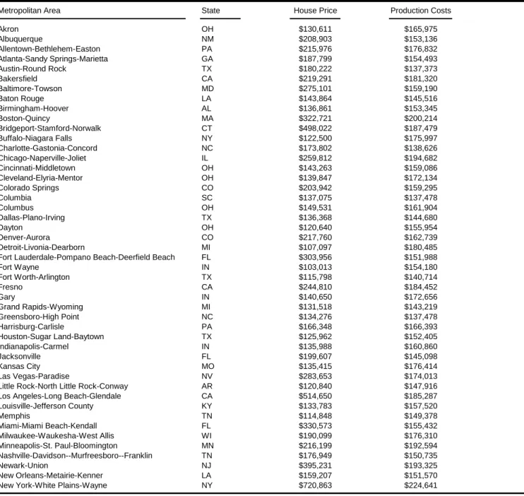
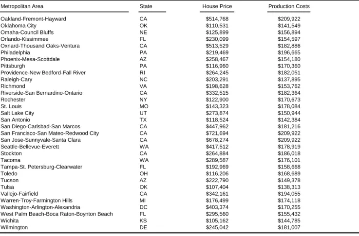
reports recent values on these variables. The first column provides 2007 prices of the median
quality home (as of 2000) in each metropolitan area. As expected, there is a wide range of
price conditions across markets. The mean value is $234,168, with a relatively large standard
deviation of $141,822. The price at the top of the interquartile range is double that at the
bottom ($275,101 versus $134,276), but even that does not capture the extreme values in the
tails. The metropolitan area in the 10th percentile of the distribution had a home price of $116,205 versus $447,962 for the area in the 90th percentile. The minimum price is $103,013, and the maximum price is $721,694.
14 The literature on whether zoning is endogenous is a lengthy one. See McDonald and McMillan (1991) and
Wallace (1988) for two early influential pieces on this topic.
15 The simple correlation between the index and the geographic constraint variables across the 78 metropolitan
areas for which we have at least one community response to the Wharton survey is -0.40. For metropolitan areas with multiple communities responding to the survey, we use the mean index value across those communities when computing this correlation. Given the strong correlation, it is not very surprising that our regression results reported below are qualitatively similar whether we use the geography- or regulation-based variable below. [The signs are reversed, of course.] Those results are available upon request, and the underlying micro data from the Wharton survey can be accessed at
http://real.wharton.upenn.edu/~gyourko/Wharton_residential_land_use_reg.htm.. We also examined data from Saks (2008), which created another index of supply-side restrictiveness based on other previous research mostly surveys. Her series also is strongly correlated with Saiz (2008) and Gyourko, Saiz and Summers (2008), but it covers many fewer metropolitan areas (about 40).
24
Minimum profitable production costs, also as of 2007, are reported in the second
column of Table 1. There are only five metropolitan areas for which this value exceeds
$200,000, and the maximum value is only $224,641.16 The mean is $166,386 and the standard deviation is a relatively small $20,032, so production costs do not vary across areas nearly as
much as prices do. Obviously, there are many markets in which prices are far above our
calculated MPPC values.
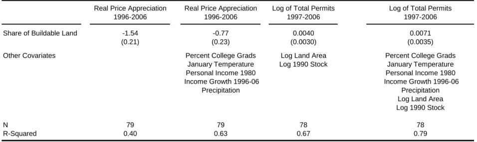
Figure 1 illustrates some of the time series variation in these data in its plot of the
average ratio of price-to-MPPC across the 79 metropolitan areas in our sample. This plot
indicates that the prices were significantly below our estimate of minimum profitable
production costs for much of the 1980s. Indeed, it was only during the recent boom that
average prices rose above construction costs.
Because the OFHEO-based repeat sales index measures appreciation on existing
homes that sell, while our estimate of production costs is for a new house, the comparison is of
prices on older homes with the costs of new product. Hence, it is not so surprising to see prices
below our estimate of MPPC. While this bias is unavoidable in any comparison of new home
costs to those based on repeat sales indexes, it does suggest that any positive gap between
prices and production costs is a conservative measure of that difference. That a large gap
clearly developed between 1996-2005 suggests that the recent boom may have been different
in certain respects.17
16 The New York metropolitan area has the highest construction costs. The four other areas with costs above
$200,000 are in the Boston and San Francisco Bay areas.
17 Obviously, we can mechanically have the price-to-cost ratio be near one in the early 1980s if we were to
assume that land constituted a lesser than 20 percent share of overall property value. But, as just noted, there is no reason to believe that this ratio could not ever be less than one. Our focus here is on the time series pattern, and we do not believe there is any reasonable chance the upward slope could be explained by errors in our underlying assumptions for the MPPC.
25
With respect to the supply side, there is considerable dispersion in Saiz’s series on the
fraction of developable land area. The sample mean for this variable is 81.6%, with a standard
deviation of 19.8%. The 10th percentile value is only 51%, compared to a 90th percentile value of 100% developable land. The most physically constrained metropolitan area is
Oxnard-Thousand Oaks-Ventura (20.7% developable land), while 13 markets are completely
unconstrained by this measure (e.g., Dayton, OH, and Wichita, KS, which are off the coasts
and have no steeply sloped land parcels within 50 kilometers of their centroids).
To gain initial insight into how house prices and quantities vary with supply elasticity
conditions over our full sample period, we estimated specifications (3) and (4) below, which
allow us to see whether national price and quantity cycles generate differential local impacts
depending upon local supply elasticity conditions. After controlling for metropolitan area and
time (year) fixed effects in the price and quantity specifications, the local effects can be seen
in the coefficients on the interaction of the developable land share variable in each market
(DevShri) with the (log) average annual national house price across the 79 areas in our sample (PriceUS,t). Specifically, we estimate
(3) log Pricei,t = α + β*Yeart + γ*MSAi + δ*(DevShri*Log[PriceUS,t]) + εi,t
(4) log Permitsi,t = α’ + β’*Yeart + γ’*MSAi + δ’*(DevShri*Log[PriceUS,t]) + ε’i,t ,
where i indexes the metropolitan areas, t represents each year from 1982-2007, and ε is the
standard error term.
The coefficients δ and δ’ indicate how price and quantity vary with the degree of
supply side elasticity, controlling for the state of the cycle (with average prices), as well as
26
-0.0228; std. err. = 0.0009), which implies that prices move much less over the national cycle
in more elastic markets. The results from equation (4) yield δ’=0.0124 (std. err. = 0.0028),
indicating that permits move much more over the national cycle in more elastic places.18 These basic results both suggest that our geographic constraint variable is proxying for supply
side conditions as we had intended and that price and quantity responses vary as our model
predicts. We now turn from these summary statistics to analyses of specific boom and bust
periods in the housing market.
IV. The 1982-1996 Cycle
The bulk of variation in housing prices is local, not national, but there still are periods
when there is enough co-movement across areas that there are recognizable national housing
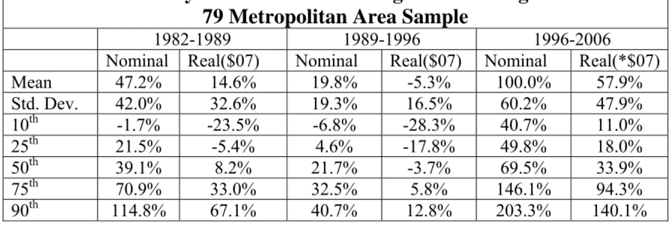
cycles. Between 1982 and 1989, three-quarters of our metropolitan areas had nominal price
growth greater than 21% over the eight year period. Inflation was relatively high during the
1980s, but real appreciation throughout the sample still averaged 14.6% over this time span.
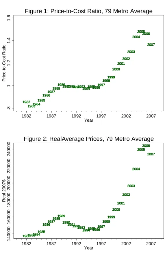
As Figure 2 shows, 1989 was the peak of average housing prices in our sample
between 1982 and 1996, so it is the natural peak of a housing cycle. Averaged across all of
our markets, prices only started to rise consistently again in 1997, so we will define the
1989-1996 period as the housing bust on the other side of this cycle. Over this latter time period,
half of our markets (40 out of 79) experienced real price declines, although barely 10 percent
(10 out of 79) experienced nominal price drops. Table 2 reports more detail on the
distribution of real and nominal price growth over time.19
18 Each specification is estimated using 2,212 observations (79 metro areas over 28 year). For the price equation,
the R2=0.91; for the quantity equation, the R2=0.85.
19 Even over this national boom-bust cycle, the bulk of year-to-year variation in price changes was local. For
27
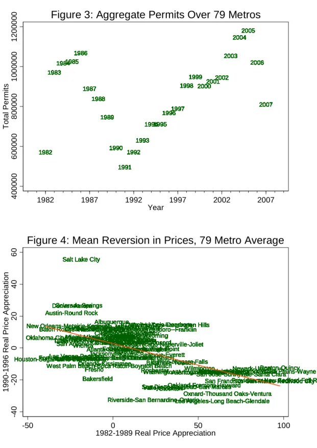
Accompanying the boom and bust of housing prices is an analogous change in housing
production. Figure 3 depicts the movement in new residential permits issue over time. The
plot is of the yearly sum of all housing permits issued in our 79 market sample. This quantity
series shows the same basic rise, decline and rise as the price series, although permits seem to
peak and trough earlier than prices. Perhaps this is because builders are able forecast price
changes, but that is an issue for future research.
Was the boom-bust cycle in housing prices a bubble or a response to fundamentals?
The national economy was doing reasonably well in the mid- to late 1980s, and interest rates
and inflation had fallen from their dramatic heights during the early 1980s. While there were
observers in the 1980s who called the price gains a bubble, the fact that real conditions were
changing dramatically made any such claims highly debatable. The best case for a bubble, at
least in some markets, was that prices fell so dramatically over a short period of time after the
boom without any obviously comparable changes in fundamentals.
For example, real prices in the Los Angeles-Long Beach-Glendale metropolitan area
rose by 67 percent between 1984 and 1989. Over the next five years, real values then declined
33 percent. We understand those who find it hard to look at Los Angeles’ prices in both 1989
and 1994 and to think that these dramatic changes in prices were actually driven by changes in
real features of southern California.20 In retrospect, it is just as possible to take the view that 1994 was unduly pessimistic as it is to take the view that 1989 was unduly optimistic. In
either case, something seems to have been amiss with standard rational pricing models, as
discussed in the Introduction.
dummies explain only 14% of the variation in housing price appreciation. Still, this implies there is a meaningful amount of national variation, possibly driven by changes in interest rates, the national economy, demographics and perhaps even nationwide beliefs about the future of the housing market.
20 See Case (1994) and Case and Mayer (1995) for early investigations into this issue for the Los Angeles and
28
While one cannot know for sure whether there was a bubble during this time period (in
at least some markets), we can determine whether the data are consistent with the key
implications of the theory presented above. One of the key predictions of our models is that
markets with highly elastic supply sides are much less likely to have ‘bubbles’. We will
examine this implication first by comparing the price gains over the 1982-1989 period in
elastic and inelastic cities. Dividing the sample in two at the median value for the share of
developable land based on geographic constraints (which is 88%) finds a large difference in
real price appreciation between the less versus more elastic areas. On average, the relatively
inelastic markets appreciated nearly five times more in real terms (23.2% versus 5.0%) than
the relatively elastic markets over this period.
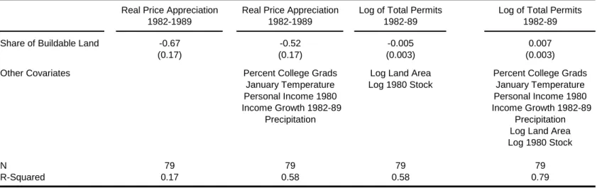
Regressing each metropolitan area’s price appreciation on our supply side proxy finds
a statistically and economically significant relationship in which a more elastic supply side is
associated with materially lower real price growth during this boom. These results are
presented in column one of Table 3. The coefficient value of -0.67 (std. err. = 0.17) implies
that a one standard deviation change in the share of developable land (which equals 20
percentage points and corresponds to a move from the 25th to 50th or the 50th to 75th percentiles of the distribution for this variable) is associated with about a 13 percentage point reduction in
real appreciation during this time period. This finding is consistent with the model’s
implication that more inelastic places will have bigger price changes during bubbles, but it is
also compatible with the view that the rise in prices in the 1980s was driven by fundamentals.
Inelasticity should produce bigger price increases, whether the inelasticity is driven by rational
29
Perhaps the biggest challenge to the implication of this simple bivariate regression is
that it reflects demand-side rather than supply-side differences across markets. To investigate
this further, we include different measures of housing demand as controls. Two amenity
variables—warmth (mean January temperature) and dryness (mean annual precipitation)—
were used. While these particular variables don’t change over time, demand for them might
have, so they provide a natural way of controlling for changes in demand. We also explored a
variety of economic variables including the share of the population with college degrees in
1980, the level of real income in 1980 as measured by the Bureau of Economic Analysis, and
the growth in that income (between 1982 and 1989 for this particular regression). The initial
level of educational achievement and 1980 income are static, of course, and should only
matter if they are correlated with changes in local economies over the 1980s. Change in BEA
real income gives us a measure of income growth.
Column 2 of Table 3 reports coefficient estimates on our supply side proxy based on a
specification that includes these demand controls. The coefficient falls to -0.52 (std. err. =
0.17), but remains statistically significant.21 There was much heterogeneity in house price growth across markets during the 1980s boom. Supply side conditions certainly do not
explain all that cross sectional variation, but they can account for a significant fraction.
Essentially, a one standard deviation change in the degree of supply-side constraint is
associated with a 0.3 standard deviation change in real price appreciation during the boom.
The last two regressions reported in Table 3 examine quantity, using the logarithm of
the number of permits between 1982 and 1989 as the dependent variable. In this case, we also
control for the logarithm of the number of homes in the area in 1980 and the logarithm of the
21 It is the economic variables, both 1980 income and its growth from 1982-1989, which are the most highly
significant and account for the attenuation of the coefficient on the developable land share. All results are available upon request.
30
land area of the metropolitan area. The logarithmic formulation means that we can interpret
these results as representing permits relative to the initial stock of housing or permits relative
to land area. In general, the relationship between the increase in the number of housing units
and the supply side proxy is less robust. The baseline regression finds a statistically
insignificant coefficient of the wrong sign (column 3). Adding in controls in the next
specification, changes the coefficient to 0.007 (std. err. = 0.003), which means that a one
standard deviation higher fraction of developable land is associated with a 0.14 log point
increase in our permitting variable, which amounts to just over 0.16 standard deviations for
that variable. Thus, there is modest evidence consistent with Proposition 3, which suggests
that more elastic places build more housing during the boom.
These results indicate that the more inelastic markets experienced a much larger price
response and a somewhat smaller quantity response during the boom period of the 1980s. The
distributional data reported in Table 4 yield more insight into the full extent of the ability of
elasticity to explain price growth variation during this time period. We split the sample into
three groups based on our developable land proxy for elasticity.22
The mean differences across the groups are very large, as expected. Being relatively
inelastic certainly is no guarantee of high price growth. One always needs strong demand for
that, and not all areas with relatively low shares of developable land have growing demand.
However, being relatively elastic really does seem to have limited the ability of a market to
experience a truly large price boom during this period. The data in Table 4 show that almost
none of the most elastic metropolitan areas experienced real price appreciation of at least 33%,
22 The most elastic third of markets is slightly larger because of lumpiness at the cut-off margin for the share of
31
which is the lower bound for the top quartile of markets. During this decade, really high price
growth over a long period of time required some type of constraint on development.
The 1989-1996 Bust
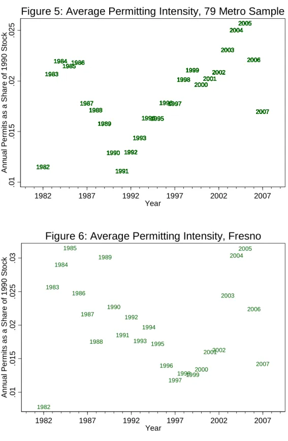
The case for interpreting 1982-1989 as a bubble in those inelastic places is made
stronger by the enormous mean reversion over the next seven years. Figure 4 plots the price
changes between 1990 and 1996 on the price growth between 1982 and 1989.23 Overall, the correlation is -59 percent. Whatever was pushing prices up in the 1980s seems to have
disappeared in the 1990s, and it is challenging to identify real economic factors that can
explain that change.
Mean differences in price appreciation between relatively inelastic and elastic areas
were much smaller during the housing bust. The forty markets with developable land shares
below the sample median did suffer larger real price declines on average, but the gap is not
particularly large: -7.9% for the relatively constrained markets versus -2.7% for the
unconstrained group. There are more extreme declines among the inelastic set. One quarter
of them suffered real price declines of at least -26%. The analogous figure for the elastic
markets is only -9%.
The regression results are not nearly as robust as those for the boom period. These are
reported in Table 5, which replicates Table 3 for the 1989-1996 time frame and then adds two
specifications. The baseline bivariate regression reported in column one yields a small,
positive coefficient. However, including the demand controls reduces its magnitude and
eliminates all statistical significance (column 2). In the third specification, we include a
control for price growth during the 1982-1989 boom period and the interaction between the
23 We use non-overlapping years to minimize the mean reversion that would be created by pure measurement