University of Nebraska - Lincoln
DigitalCommons@University of Nebraska - Lincoln
Sociology Department, Faculty Publications
Sociology, Department of
Spring 2015
Global Network Inference from Ego Network
Samples: Testing a Simulation Approach
Jeffrey A. Smith
University of Nebraska–Lincoln, [email protected]
Follow this and additional works at:
http://digitalcommons.unl.edu/sociologyfacpub
Part of the
Sociology Commons
, and the
Statistical Methodology Commons
This Article is brought to you for free and open access by the Sociology, Department of at DigitalCommons@University of Nebraska - Lincoln. It has been accepted for inclusion in Sociology Department, Faculty Publications by an authorized administrator of DigitalCommons@University of Nebraska - Lincoln.
Smith, Jeffrey A., "Global Network Inference from Ego Network Samples: Testing a Simulation Approach" (2015).Sociology Department, Faculty Publications. 258.
Copyright © Taylor & Francis Group, LLC. Used by permission. Published online March 31, 2015
Global Network Inference from Ego Network
Samples: Testing a Simulation Approach
Jeffrey A. Smith
Department of Sociology, University of Nebraska–Lincoln, Lincoln, Nebraska, USA
Abstract
Network sampling poses a radical idea: that it is possible to measure global network struc-ture without the full population coverage assumed in most network studies. Network sampling is only useful, however, if a researcher can produce accurate global network estimates. This article explores the practicality of making network inference, focusing on the approach introduced in Smith (2012). The method uses sampled ego network data and simulation techniques to make inference about the global features of the true, un-known network. The validity check here includes more difficult scenarios than previous tests, including those that go beyond the initial scope conditions of the method. I exam-ine networks with a skewed degree distribution and surveys that limit the number of so-cial ties a respondent can list. For each network/survey combination, I take a random ego network sample, run the simulation method, and compare the results to the true values (using measures of connectivity and cohesion). I also test the method on local measures of network structure. The results, on the whole, are encouraging. The method produces good estimates even in cases where the degree distribution is skewed and the survey is strongly restricted. I also find that is it better to not truncate the survey if possible. If the survey must be restricted, the researcher would do well to infer the missing data, rather than use the raw data naively.
Keywords: exponential random graph model (ERGM), simulation, social networks 1. Introduction
Network studies have traditionally been restricted to relatively small, bounded settings with full information on the population of interest. Network structure is easily measured under these ideal conditions, opening up questions about connectivity (i.e., disease/infor-mation spread), group divisions and cohesion (Moody & White, 2003; Shwed & Bearman, 2010; Mucha, Richardson, Macon, Porter, & Onnela, 2010; Adams, Moody, & Morris, 2013). In many cases, however, it is impractical to collect full network data on the population of interest (Frank, 1971; Koskinen, Robins, Wang, & Pattison, 2013). The network may be too large and the resources available too small to interview everyone, while electronic informa-tion on social ties may be unavailable. This is especially true of comparative network stud-ies. A study on social integration, for example, would need to measure network cohesion
125
across many neighborhoods, villages, or schools (Sampson & Raudenbush, 1997; Brown-ing, Cagney, & Iveniuk, 2012; Verdery, Entwisle, Faust, & Rindfuss, 2012). Traditionally, a researcher would have to collect full network data in every context, a tall order by any sur-vey method standard.
A small but growing literature on network sampling has raised the possibility of making inference on network structure without the full coverage assumed in most network studies (Frank, 1978; Handcock & Gile, 2010; Koskinen, Robins, & Pattison, 2010; Krivitsky, Hand-cock, & Morris, 2011). Using sampled network data eases the burden of data collection con-siderably but also raises difficult inference problems. Global network measures depend on all of the ties among individuals while sampled data, by definition, only provide sampled bits of the network. As a solution to this inferential problem, recent work has offered sim-ulation techniques as a means of making inference from sampled network data (Lee, 2008; Morris, Kurth, Hamilton, Moody, & Wakefield, 2009; Smith, 2012; Merli et al., 2015).
This article examines the practical application of simulation to network inference. I fo-cus on the method proposed in Smith (2012). The method uses ego network data to make inference about global network structure. Individuals are first randomly sampled from the population; they then answer questions about themselves (e.g., demographic information) and the people they are socially connected to, such as friends or confidants (Marsden, 1987; Smith, McPherson, & Smith-Lovin, 2014). Respondents also report on the ties between their named alters. The method uses this data to simulate networks consistent with the sampled, local information. For example, the survey yields an estimate of the degree distribution, or the number of ties per person, and the simulation is conditioned on this information. Finally, the method calculates the global statistics of interest on the generated networks, such as average distance, modularity, or cohesion. The approach has great potential as in-dependently sampled data are easy to collect and can be incorporated into existing surveys. There is also empirical reason to be optimistic, as the method performed quite well in a series of validity tests (Smith, 2012). These tests, while employing a large number of net-works, adhered strongly to the initial scope conditions of the method. The original tests were limited to networks based on strong tie relationships, where individuals have a rel-atively small number of social ties and can easily enumerate them within an ego network survey. Based on this strong tie assumption, the tests were limited to low-degree networks and assumed full information about respondents’ social contacts.
The goal of this article is to apply the approach to a wider set of contexts, even if those contexts fall outside the bounds initially specified by the method. For example, ego net-work sampling may yield biased estimates when the netnet-work has a skewed degree distri-bution so that a few individuals have a disproportionally large number of ties (Barabasi & Albert, 1999; Gould, 2002). High degree individuals have a large impact on network struc-ture but are not any more likely to be sampled (as it is a random sample of the population). Thus, the sampling scheme may miss important nodes in highly skewed networks, lead-ing to potential biases.
Additionally, surveys will often restrict the amount of information that is collected. A typical survey will limit the number of social contacts a respondent can name. This is done for practical reasons, for example, to reduce respondent fatigue and the cost of the survey (Burt, 1984). This will result in a truncated degree distribution, however. Even if one is lucky
enough to sample a high degree node, one would still have an inaccurate measure of their degree—as there is only information up to the truncated amount (say, 10 ties).
Here, I drop the simplifying assumptions of previous tests and show how degree skew and degree truncation affect the bias in the estimates. Is the method appropriate for all lev-els of degree skew and survey truncation? More generally, what should a researcher do when faced with less than ideal conditions? I begin the article with a background section on ego network sampling and the simulation approach. I then discuss the experimental setup used to test the method, before moving to the results.
2. Ego Network Sampling
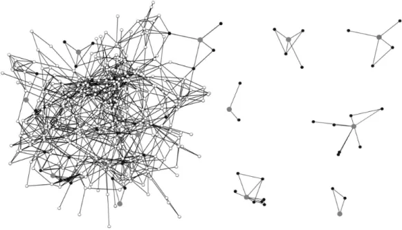
Figure 1 summarizes the problem of network sampling. Panel 1 in Figure 1 plots a typ-ical (hypothettyp-ical) network structure. We can assume that the network represents friend-ships among adolescents in a school. A researcher would normally collect information on all nodes, here adolescents, and all ties between nodes in the network. This information can be used to characterize the topology of the network. For example, the paths between nodes are easy to enumerate when the network is complete. Substantively, the path structure yields a measure of diffusion potential, where lower average distance and higher levels of connec-tivity equals higher probabilities of global diffusion (Watts, 2002; Centola & Macy, 2007).
But what if it is impractical to collect information on every individual in the network? In such cases, it is necessary to make inference from a sample. There are many ways to sample a network, such as snowball and subgraph approaches (Thompson & Frank, 2000; Good-man, 2011), but I focus on the simplest possible option, the ego network sample (Marsden, 1988).
In Panel 1, I have highlighted a hypothetical ego network sample from the full network. The grey nodes represent the randomly sampled respondents from the set of all individu-als in the network. The white nodes represent the nonsampled respondents, and the black nodes are the friends of the respondents. The black nodes (here the friends of the respon-dents) are not interviewed, but we receive information about them indirectly through the respondent’s reports on them. For example, we would know if the friends of the respon-dents are themselves friends (Louch, 2000). The sample thus offers information on the grey nodes and the black nodes, leaving independent bits of the network. These sampled sub-structures are plotted separately in Panel 2. The sampled parts of the network cannot be connected, as ego network surveys do not collect identifying information on the named friends (i.e., the black nodes).
Ego network sampling poses more than a missing data problem (Kossinets, 2006; Bor-gatti, Carley, & Krackhardt, 2006; Smith & Moody, 2013). It is a problem of statistical infer-ence, where almost all of the network information must be “filled in.” The question is how we can take information on the respondents and their friends, or these disconnected, rep-resentative pieces of the network, and make inference about the entire graph (as one can-not simply trace out the paths between nodes anymore).
2.1. Background on Simulation Approach
Smith (2012) provides a simulation solution to the problem of network inference. The method takes independently sampled ego network data, like that in Figure 1, and makes inference about the entire network structure.1 The simulation approach rests on a simple
premise: that one should generate networks consistent with the local information found in the sampled data. A simulated network consistent with the local information should have similar macro features as the real network. The method ultimately works well because it utilizes so much of the information embedded in the network survey.
As with most surveys, an ego network sample will provide information about the demo-graphic characteristics of the respondents, or the sampled grey nodes in our example net-work. Individuals may be asked about their gender, race/ethnicity, education, age, and so forth. This information is useful in the simulation because it yields the demographic com-position of the network.
An ego network survey will also ask respondents to name their alters, or those individ-uals to whom they are socially connected. The alters are defined as friends in Figure 1. The
1 It is important to note that the method is only appropriate for well defined populations with a sam-pling frame. The population of interest is thus assumed to be nonhidden (i.e., not female sex work-ers or drug injectors), and the size of the population is assumed to be known. The method also assumes that the relationship of interest is symmetric, so that if i nominates j, then j nominates i.
node on the top right of Panel 2 would list four alters, or have degree 4, while the node on the bottom right would list two alters, or have degree 2. This yields an estimate of the de-gree distribution, equal to the number of alters per respondent. The alter list also offers in-formation on differential degree, or the mean degree by demographic group. This can be inferred from the data because there is information on degree and the demographic char-acteristics of the sampled respondents. The highly educated may have more ties than those with less education (e.g., Lizardo, 2006; McPherson, Smith-Lovin, & Brashears, 2006).
Ego network samples also provide information on the demographic characteristics of the alters. For example, for the top-right respondent, a researcher may ask about the race, gender, and age of the four friends. Respondents are often asked to report on only a subset of their alters. A respondent may list 15 friends but only be asked about the demographic characteristics of the first five (e.g., Marsden, 1987). This is done to limit respondent burden.2
The alter demographic data are important for the simulation because they offer informa-tion on homophily, or the tendency for demographically similar individuals to be socially connected (McPherson, Smith-Lovin, & Cook, 2001; Smith et al., 2014).3 The data show if
respondents and their alters have the same race/gender/age/etc.; we can thus ask if there is strong homophily along religious lines, for example (Cheadle & Schwadel, 2012). The data also capture the pattern of ties among demographic groups (Rosenfeld, 2008). Thus, we can ask if ties between Whites and Asians are more likely than ties between Whites and Blacks (Qian, 2002; Qian & Lichter, 2007).
Finally, ego network data provide information on the ties between alters. Respondents are asked about the ties that exist between alter 1 and 2, 1 and 3, 2 and 3, and so on. Again, the surveys are often limited to curtail respondent burden. A respondent may be asked about a subset of all ties that exist between alters (i.e., the ties that exist among the first five friends). For our top-right respondent, we would know that two of their friends are tied to-gether; we would also know that these two friends are not tied to the other two friends, who are not tied to each other. The alter–alter tie data offer information about the local struc-tural patterns in the network. Are individuals tied to the respondent also tied to each other, so a friend of a friend (the respondent) is also a friend (Goodreau, Kitts, & Morris, 2009)?
One of the contributions of Smith (2012) was its unique characterization of the alter– alter tie data. Past work has generally relied on density (the number of ties amongst al-ters divided by the total number of possible ties) to measure the structure of ego networks (Fischer, 1982; Mardsen, 1987; although see Louch, 2000, for an exception).4 Unfortunately,
this does not offer a precise enough measure for the purposes of the simulation: many net-works with the same local density have very different global structures (Smith, 2012). As
2 It can be quite tedious to describe the demographic characteristics of many alters along many de-mographic dimensions.
3 One can estimate the strength of homophily as one knows the characteristics of the respondents and the respondents’ alters.
4 This is largely because ego network data provide biased estimates for many typical triadic mea-sures; such as global transitivity, defined as the proportion of two-step paths where there is also a one-step path (Soffer & Vazquez, 2005; Bansal, Khandelwal, & Meyers, 2009). Thus, for our top-right respondent, there is one tie out of a possible six.
the networks are generated from the local information, it is important to have a discerning measure of local structure.
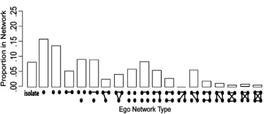
Smith (2012) offered an alternative measure of ego network structure, one that encapsu-lates all of the information available from the sampled data. The basic idea is to form a dis-tribution of ego network configurations from the alter–alter tie data (see Holland & Lein-hardt, 1976, and Middendorf, Wiggins, & Honig, 2005, for similar intuition). Figure 2 plots a hypothetical ego network configuration distribution. The histogram is limited to four al-ters for the sake of space considerations, but the actual distribution is not limited by size. Each respondent is placed into a distinct structural type, based on the size of the ego net-work and the pattern of ties between alters. For example, our top-right respondent would fall into the 10th configuration from the left (four alters with one tie between them), while the top-left respondent would fall into the 11th configuration.
Formally, let Yp be a square matrix of dimensions m × m, consisting of the alters in the ego network of respondent p. Define Ypij = 1 if a tie exists between alter i and j. The ego net-work configuration can then be defined by the unique combination of:
1. Sizep = m
2. (di)p = Ypi+ , where di is the degree of alter i
3. Tp = ∑ Ypij * Ypjk * Ypik , where t is set of all triads in Yp t
A distribution of ego network configurations offers a more discriminating measure be-cause it fully captures the structural features of the ego networks. Ego networks of the same size and density can exhibit very different structural patterns, but this is obscured us-ing traditional measures. For example, there are four distinct configurations with four al-ters and three ties between alal-ters. Substantively, the forces that constrain the real network, such as transitive closure (where a friend of a friend is a friend) will also constrain the ego network configurations, making it more likely that the simulated network will reflect the properties of the true network (as the simulated networks are conditioned on the ego net-work configurations).
Figure 2. Example ego network configuration distribution. Note: This figure is a based on a hypotheti
-cal ego network configuration distribution. Ego is not included in the ego network types. I only include ego network types of size four or less to make the figure legible.
The simulation generates full networks that are consistent with the information ex-tracted from the ego networks: the degree distribution, differential degree, homoph-ily, and the ego network configuration distribution. A network consistent with this local information should have similar global features as the true network—as the sim-ulated networks are heavily constrained by the empirical data. The method draws on two models to simulate the networks, exponential random graph models (ERGMs) and case control logistic regression. I briefly discuss both models before moving to the de-tails of the approach.
2.2. ERGM
ERGMs offer a statistical approach to modeling network data. The model form is quite general, and can be used to test hypotheses about network structure/formation (Holland & Leinhardt, 1981; Frank & Strauss, 1986; Wasserman & Pattison, 1996; Snijders, Pattison, Robins, & Handcock, 2006; Handcock, Goodreau, Hunter, Butts, & Morris, 2008). Formally, we can define a network, Yij, over the set of nodes N (N = 1, 2, … n), such that Yij = 1 if a tie exists and 0 otherwise. Let y be the observed networks. Y is then a random graph on N, where each possible tie, ij, is a random variable. An ERGM will model the Pr(Y = y). The “independent variables” are counts of local structural features in the network (Robins, Sni-jders, Wang, Handcock, & Pattison, 2007; Goodreau et al., 2009), such as the volume of ties, homophily (e.g., the number of ties that match on race), or transitivity (e.g., the number of transitive triads). The model can be written as:
P(Y = y) =
exp
(
θ
T
g(y)
)
κ(θ)
where g(y) is a vector of network statistics, θ is vector of parameters, and κ(θ) is a normal-izing constant.
Typically, ERGMs are used to test hypotheses about the formation of the network, but it is also possible to simulate networks from an underlying model. The coefficients cap-ture the effect of different local processes on the formation of the network. We can then use those coefficients to predict the presence of ties between individuals in a constructed network.
Prior to a simulation, a researcher must specify the model terms and coefficients used to generate the network. The model should be specified with the end goal in mind. In this case, the goal is to simulate networks consistent with the local network information. The model terms should reflect the information available from the ego network sample, while the coefficients should generate networks with the right local features.
2.3. Case Control Logistic Regression
The second model, case control logistic regression, is used to estimate the initial coef-ficients for the ERGM (Smith et al., 2014). The case control model is specifically used to estimate the coefficients for the homophily terms. The model is also used to adjust the
homophily coefficients during the simulation (see Merli et al., 2015, for an example). Case control models are often used in medical research to study rare conditions that are diffi-cult to capture through random sampling (Breslow & Day, 1980). The models compare the cases, a set of individuals with the “disease” (e.g., cancer), to the controls, a set of individ-uals without the “disease.” A case control model is ideal for ego network data because the sample captures the rare event of interest, the social relationships between actors. The cases are all respondent–alter pairs, or those pairs with a known social relationship (the “disease” of interest). The controls represent a random sample of pairs that do not have a known so-cial relationship. This is formed by randomly pairing the sampled respondents together, capturing random mixing in the population.
The case control model compares the cases to the controls on some behavior or con-dition of interest (e.g., smoking). Here, the concon-dition of interest is the sociodemographic distance between individuals in a pair. For numerical variables, like age, this is measured as the absolute distance between i and j. For categorical variables, like race or religion, distance is measured as a matching term (are i and j the same race?) or a set of dummy terms, describing the rate of contact between all categories (e.g., what is the rate of so-cial contact between Whites and Blacks, Whites and Asians, and so forth?). The sociode-mographic distance between the respondents and alters, or the cases, is compared to the sociodemographic distance between randomly paired respondents, or the controls. The model thus compares the sociodemographic distance observed in the data to that expected under random mixing in the population (Smith et al., 2014). The model is a simple logis-tic regression, where the 1s are the respondent–alter pairs and the 0s are the random re-spondent pairings. Formally
ln
(
p(Y)
)
= θD
1 – p(Y)
where Yij is the presence or absence of a tie, Dij is the sociodemographic distance between i and j for each dyad, and θ is the vector of coefficients.
The case control model is useful because of its flexible form: The controls are constructed independently from the cases, making it easy to alter the comparison. This makes the ini-tial estimation straightforward, and, more importantly, makes it possible to update the co-efficients during the simulation itself.
3. Methods Overview
The simulation approach draws on both models to generate networks consistent with the sampled information. I describe the approach here in some detail but see Smith (2012) for a complete discussion.
The method has three basic parts: first, summarizing the sampled data prior to the sim-ulation; second, setting up the simsim-ulation; and third, simulating the full networks. The first part gathers information from the sampled ego networks, while the second and third parts generate full networks that are consistent with the local, sampled information. I assume, when describing the method, that the survey has collected demographic information on
both the respondents and alters. I also assume that there is information on the number of alters and the ties between alters.
The method begins by calculating the degree distribution from the sampled data. The degree distribution is taken directly from the sampled data itself. Thus, the proportion of respondents with 0, 1, 2, etc., alters is used as the estimate of the degree distribution. This is a quite simple approach, but it is also possible to use more complicated, model-based methods when estimating the degree distribution (e.g., Zhang, Kolaczyk, & Spencer, 2014). Thus, one could estimate the generating function of the degree distribution, take draws from that model, and use that as the degree distribution for the network. This would serve to smooth out the distribution from the sample. In the case of a truncated survey design (e.g., where only 10 names are collected), it will be particularly important to use a model-based approach—as the sample degree distribution will not offer a good approximation of the true degree distribution.
As a second step, the method calculates the ego network configuration distribution from the sampled data (see formula and discussion above).
The next series of steps sets up the simulation. Here, the method first generates a work of size N with the correct degree distribution, already calculated from the ego net-work data.5 The size of the population is assumed to be known.6 The method then assigns
demographic characteristics to the nodes in the simulated network. A sampled respondent is first selected at random; a node from the seeded network is then selected with the same degree as the sampled respondent. The selected node is assigned all of the characteristics of the selected respondent, such as race, gender and education. This maintains differential degree in the simulated network, as demographic groups with high average degree in the sample will also have high average degree in the network (as characteristics are assigned to nodes based on degree).7 The initially simulated network will thus have the right size,
degree distribution, demographic composition, and differential degree (where everything but size is based on the sampled data).
The method then specifies an ERG formula to simulate the full network from. The ERG formula specifies which local features are used to form the full network of interest. The terms in the model should reflect all of the local information available from the ego network
5 This initial simulation can be done within an ERGM framework or using a stub-based algorithm (Newman, Strogatz, & Watts, 2001; Viger, Latapy, & Wang, 2005).
6 See Pattison, Robins, Snijders, and Wang (2013) for approaches that do not require the size of the network to be known.
7 It is important to note that the number of people in the simulated network is larger than the number of sampled respondents. This means that a sampled respondent may be seeded multiple times in the simulated network. This is unlikely to cause problems, however, as the network ties are prob-abilistically determined; thus, nodes in the simulated network with the exact same set of charac-teristics need not be tied together. Or, there is no definitional reason that a node seeded multiple times will have to be tied to herself. Any nodes with similar characteristics will have a high prob-ability of being tied together. More substantively, it may be the case that many people have the same race and grade in a school; in which case the simulation does not deviate far from the empir-ical setting. Future work could, however, explicitly deal with this duplication of nodes by mod-eling how the characteristics go together, rather than simply drawing them from the data itself.
sample: differential degree, homophily, and the ego network configuration distribution. There are two steps here: first, determining which terms should be included; second, cal-culating the initial coefficients for those terms.
The model will include homophily terms for each demographic dimension available in the data. The homophily terms take the form of an absolute difference if they are continuous, like age. Thus, we would be interested in the absolute age difference between respondents and their alters. The method uses a mixing matrix to capture homophily if the terms are cat-egorical, like race or gender. The mixing matrix reflects the number of social ties between each category. For example, the terms for race may include Black–Black, Black–Hispanic, White–White, and so forth, capturing the number of social ties between each racial group.
The model also includes a term for geometrically weighted edgewise shared partner (GWESP) distribution. GWESP counts the number of shared partners that i and j have (as-suming i and j are themselves tied), or the number of common associates. GWESP substan-tively captures higher order transitivity in the network, or the tendency for local clusters to emerge. The GWESP term is designed to capture the ego network configuration distri-bution. GWESP is an appropriate choice as it mirrors many of the structural features of the ego networks. For example, the shared partner distribution in an ego network is the same as the degree distribution of the alters (from the point of view of the respondent), a key component in defining the ego network configurations.
The method then sets the initial coefficients for each term. The homophily coefficients are estimated using case control logistic regression (Smith et al., 2014). The GWESP coefficient, in contrast, cannot be easily set prior to the simulation; this is the case as it is not possible to analytically solve for the value that will yield the right ego network configuration dis-tribution. Rather, GWESP is set at an initial value and is updated during the simulation as the method looks for a better fitting network.8 The degree distribution and differential
de-gree (specified while seeding the network) are also maintained throughout the simulation. The framework takes the initial ERGM (coefficients, terms, and constraints) and simu-lates a network. The simulated network is then checked to make sure the homophily rates are correct. The homophily coefficients (and network) are updated if any discrepancies are found. The simulated networks may have incorrect homophily rates because the initial case control model only includes homophily terms. The initial homophily coefficients are thus unconditioned. The simulated networks, however, have a nonzero GWESP coefficient, mak-ing the homophily coefficients biased when simulatmak-ing the networks.
Formally, the case control model is used to update the coefficients, comparing the true rates of homophily to those in the simulated network and adjusting accordingly. Coeffi-cients are decreased if there are too many ties among groups and increased if there are too few. The method takes the tied dyads from the simulated network and the respondent–alter dyads from the sampled data and forms a combined dataset. This dataset includes the de-mographic characteristics of each person in the dyad. The dataset also includes a 0/1 vari-able: equal to 0 if the dyad comes from the simulated network and 1 if the dyad comes from
8 The method calculates a starting value by estimating a dyadic independent ERGM on the ego net-works. It is also possible to use other terms than GWESP.
the empirical sample. The method then runs a logistic regression, predicting the 1s as a func-tion of the sociodemographic distance between individuals in the dyads. Substantively, the logistic regression compares the sociodemographic distance from the empirical sample (i.e., between respondents and alters) to the sociodemographic distance between tied individuals in the simulated network. For example, for categorical variables, a positive coefficient means that the simulated network has too few ties between those groups. The estimated coefficients are then added to the original homophily coefficients. This adjusts the original homophily co-efficients up or down, depending on the bias in the simulated network. The network is then updated based on these new coefficients. (See Smith, 2012, for more formal details.)
The simulated network is then evaluated on how well it captures the ego network con-figuration distribution from the sampled data. The ego network concon-figurations found in the simulated network are compared to the observed distribution in the sample using a chi-square value.9 Specifically, the chi-square calculation has two parts: first, calculate the ego
network configuration distribution from the simulated network, and second, compare the ego network configuration distribution from the simulated network to the distribution from the sampled data (calculated prior to the simulation). We can write the chi-square value as
n
∑ (O
i– E
i)
2 i=1E
iwhere Oi is the observed frequency in the simulated network, Ei is the frequency found in the sample, and n is the total number of possible ego network configurations. The chi-square value will be large, and the fit poor, if is there is a large difference between the true distribution and the distribution from the simulated network.
The coefficient on GWESP is then updated to find a better fitting network, if possible. A better fitting network will have ego network configurations that match the true distribu-tion more closely, condidistribu-tion on the other local features in the sampled data. As the simula-tion looks for a better fitting network, it is necessary to compare the homophily rates in the simulated network to the rates in the sampled data.
The ego network configuration distribution thus serves as the benchmark by which to judge the simulated networks. The question is what coefficient on GWESP will yield a net-work with the lowest chi-square value. The minimization process begins by simulating a sample of networks with different values for GWESP; the values are set above and below the initial value for GWESP. The method then adjusts the simulated networks for any ho-mophily bias and calculates the chi-square value, comparing the true ego network configu-ration distribution to the distribution in the simulated network. The coefficients on GWESP and the chi-square values are then used to fit an OLS regression. The chi-square values are regressed on linear and quadratic terms of the GWESP coefficients. Formally
χ
i2= β
0
+ β
1(G
i) + β
2(G
i)
29 A good fit means that the ego network configurations in the simulated network are found at the same rate as in the sampled data.
where χi2 is the chi-square value for network i, and G
i is the coefficient on GWESP for net-work i. The regression coefficients are then used as inputs into an optimization routine; the method uses the Nelder-Mead algorithm to find the GWESP coefficient that yields the low-est chi-square value. The coefficient that minimizes the equation is then used as the start-ing point for the next iteration of the simulation. This process is repeated until it is impos-sible to improve the fit by changing the GWESP coefficient and updating the homophily coefficients. In general, the simulation rests on a kind of approximated likelihood ratio test: The coefficients are updated to find a more likely network, where a network is considered more likely if the ego network configuration distribution more closely matches the true dis-tribution from the sample.
In the end, the simulation will yield a network with the same local properties as the sam-pled ego network data: It will match the degree distribution, differential degree, homoph-ily and the ego network configuration distribution. The researcher can then calculate the global statistics of interest on the generated network.
4. Analytical Setup: Testing the Method
The key question is how closely the method reproduces the true network. A test of the simulation approach has four steps: first, select a known, complete network as a test case; second, take an ego network sample from the known network; third, use the simulation approach to estimate network properties of interest; and fourth, compare those estimates to the true values on the known network.
I use this general setup to examine two validity threats to the approach: skewed degree distributions and truncated survey designs. A degree distribution is skewed when a few nodes have very high degree relative to the rest of the population. A network with a skewed degree distribution may be difficult to simulate accurately. A random sample of the popula-tion could miss the high degree nodes (because they are not any more likely to be sampled than anyone else), but these actors are disproportionally important for network structure. Those with high degree are connected to many people and are likely to connect disparate parts of the network. A researcher is likely to underestimate the global connectivity of the network if the sample misses these important hubs.
Similarly, survey designs will often limit the number of alters a respondent can name. A person with 15 friends may only be able to list five or 10. This is done to limit respondent bur-den, but it also makes it hard to infer the true degree distribution. Even if a researcher was for-tunate and sampled a high degree node, they would not discover this information if the sur-vey was limited to a small number of alters. This will be especially consequential for networks based on weaker relationships, where an individual can maintain a large number of social ties.
I incorporate varying levels of degree skew and survey truncation into the larger frame-work for testing the method. Degree skew and truncation are the only variables allowed to vary during the analysis (along with the researcher’s response to these problems). I divide the discussion into two parts. I first describe aspects of the test that are held fixed through-out the analysis. I divide this discussion into three subsections: the known network; the sample from the known network; and the global network properties of interest. I then de-scribe the experimental setup itself, describing how degree skew and survey truncation are allowed to vary. I also discuss what steps the researcher can take to limit the level of bias.
4.1. Known, Complete Network
I use networks simulated from an underlying ERGM as the basis for the test.10 I
gen-erate networks from a known model (as opposed to using an empirical network) because simulated networks can be fully controlled, making it easier to represent the different fea-tures in the experimental setup (Borgatti et al., 2006). The generated networks are 500 nodes and the model includes terms for transitive closure and homophily on grade and race. The composition of the generated networks and the coefficients in the ERGM are modeled after an empirical Add Health network (e.g., Haynie, 2001; Moody, 2001; Schaefer, Kornienko, & Fox, 2011). The network is also assumed to be symmetric. The degree distribution is al-lowed to vary by experimental condition (see below), while all other features are held con-stant throughout the analysis. The networks thus have empirically realistic features but are easily manipulated to satisfy the test conditions. I will assume, for ease of exposition, that the generated networks come from a school setting, representing adolescent friendships. 4.2. Sampling Setup
I assume that a 20% ego network sample is taken from the full, known networks. The hypothetical survey has 100 “respondents” and is assumed to collect the following infor-mation: the number of alters per respondent, the race and grade of the respondent, the re-spondent’s report on the race and grade of the alters, and the rere-spondent’s report on the ties between alters. The survey is hypothetical in the sense that no respondents are actually interviewed and all information on the sampled nodes is taken from the true network.11
For both the alter–alter ties and the demographic information, the respondent “reports” on only five alters. In this way, the hypothetical survey mimics real data collection limita-tions—where respondent fatigue is a concern. Since this is not an actual survey, the five al-ters are randomly selected from the set of all alal-ters for that node (acting as the five alal-ters they chose to report on).
4.3. Network Properties of Interest
I include five global measures in the test: component size, defined as the largest set of nodes connected by at least one path; bicomponent size, defined as the largest set of nodes connected by at least two independent paths (Moody & White, 2003); mean distance, defined as the length of the shortest path between nodes (on average); and reachability, defined as the proportion of nodes reachable X steps out into the network (on average). I include two measures of reachability, one going three steps out into the network and the other going five steps out into the network. I also include results for the full distance distribution, de-fined as the proportion of dyads that are 0, 1, 2, etc., distance apart. These represent typical
10 Note that the simulations here are not part of the inferential process, but are rather used to gener-ate networks to make inference about.
11 Specifically, because this is a hypothetical survey, we do not have the respondent’s report on alter race, gender and the alter–alter ties. I thus use information from the actual network as a (perhaps idealistic) proxy of what a respondent would report for the characteristics of their alters. Similarly, the number of alters is their degree from the true network.
measures of global connectivity and diffusion potential in a network. Bicomponent size of-fers a measure of cohesion, showing how robust the network is to disconnection.
I also include a set of more local network measures, as many researchers will be inter-ested in local network structure. The local measures include: the mean, standard deviation and skew of the degree distribution, density, the number of two-paths, transitivity, the pro-portion of open triads, the propro-portion of closed triads, and the geometrically weighted dyad shared partner (GWDSP) distribution. The degree distribution is measured as the propor-tion of people with degree 0, 1, 2, and so forth. The mean, standard deviapropor-tion and skew measures are summaries of the full degree distribution. Density is defined as the num-ber of observed ties in the network divided by the numnum-ber of possible ties. A two-path ex-ists between i and j if there exex-ists a tie between i – k and k – j; the summary measure is the count of two-paths in the network. Transitivity is the proportion of two-step paths where there is also a one-step path. The proportions of unclosed and closed triads summarize the triad census: an unclosed triad is defined as a triad with two ties (as the networks are un-directed), while a closed triad is defined as a triad with three ties. The dyad shared part-ner distribution is defined by the number of nodes that i and j are both connected to, or the number of shared friends. This leads to a distribution of shared partners (at the level of the dyad), which is summarized as a geometrically weighted summation. I set alpha to 1 when calculating the summation.
5. Experimental Setup
Three variables are manipulated in the experimental setup: the baseline networks, rang-ing from low degree skew to high degree skew; the survey design, rangrang-ing from no trunca-tion to strong truncatrunca-tion; and the researcher’s response to truncatrunca-tion, ranging from nothing to inferring the missing data. There are three conditions for each experimental variable, leav-ing a 3 × 3 design and nine data points overall. The experiment captures the negative effect of degree skew on the estimates; it also recognizes that the rate of degradation is conditioned on the available survey information and the researcher’s response to the survey conditions. 5.1. Varying the Networks of Interest
The three test networks range from low degree skew to high degree skew. Figure 3 plots the degree distributions for the three baseline networks. The top-degree nodes range from 26 in the low skew network to 47 in the medium skew network to 75 in the high skew net-work. Similarly, the skew in the degree distribution increases as we move down the plot. The bulk of the degree values are still between 0 and 20 in the medium and high skew net-works, but the tails are much longer. One or two people now collect a much larger propor-tion of the total number of ties.
The method was initially designed with strong tie relationships in mind. Relationships based on trust and emotional support, such as close friendships or confidants, require large time/energy investments; this limits the number of ties an individual can maintain. Net-works based on strong tie relationships are appropriate for the method precisely because it is difficult to maintain many strong ties. The degree distribution will have a short tail, and it is relatively easy to list of all one’s social contacts—minimizing problems of fatigue and the
necessity of truncating the survey. This makes the high skew network a particularly diffi-cult test. The high skew network includes individuals with 75 ties, and represents networks based on weak social relationships, such as acquaintanceship. The question is whether the method will work even in situations where individuals maintain a large number of ties.
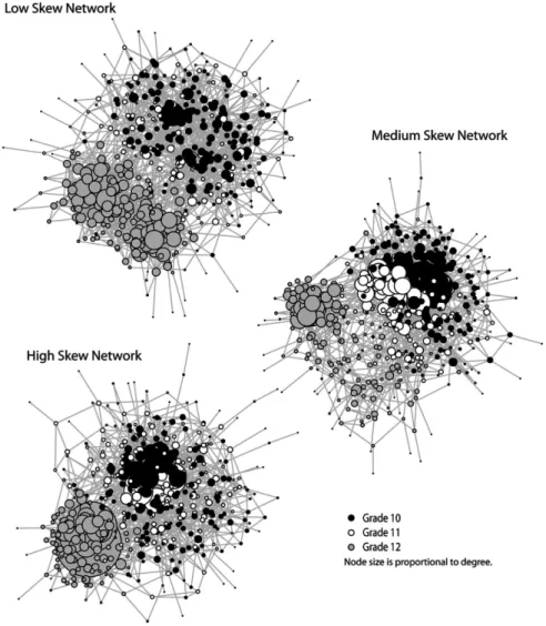
I have plotted the three networks in Figure 4. The nodes are colored according to grade and sized according to degree; larger nodes have higher degree. It is clear in all of the net-works that the system is organized along grade levels. Grade 12 is separated from Grade 11 and Grade 10, which form a loosely connected group of their own. It is also clear that the top degree in each network increases as move from the low skew network to the high skew network. In the high skew network, the highest degree node is found in Grade 12. This node plays a large role in connecting the Grade 12 students to each other. The high skew network exhibits lower average distance and higher reachability than the low/me-dium skew networks.12
Figure 3. Degree distribution for test networks: Low to high skew.
12 Note that even though the top degree is larger in the high skew network, homophily is still quite important in organizing the social structure of the school.
5.2. Varying the Survey Design
Given the networks of interest, I also vary the amount of information assumed to be col-lected in the ego network survey. The experimental design includes three survey types: strong truncation, medium truncation and no truncation. The surveys vary how many friends the respondents are allowed to name—up to 10 friends (strong truncation), up to 25 friends (medium truncation), or no limit (no truncation). For example, if a sampled node has 30 friends in the full network, we would know about the first 10 under strong truncation, the first 25 under medium truncation, and all 30 under no truncation.13 In the simulation
Figure 4. Networks used to test simulation method.
13 Even in the low skew network there could be differences across survey conditions as many indi-viduals have more than 10 friends. Across all survey conditions, I assume that alter demographic information is only recorded for five alters.
experiment, a node with degree 30 would appear in the sample as a node with degree 10, 25, or 30, depending on the level of truncation.
5.3. Varying the Researcher’s Response to Survey Truncation
The final variable in the experimental design is the researcher’s response to the survey. Surveys will often truncate the alter listing to limit respondent burden. A researcher may react in a number of ways to this (potential) validity threat. The experiment varies the re-searcher’s response to reflect different courses of action.
As a baseline, the researcher could do nothing, taking the data as is. Here, if the survey truncates the alter listing at 10, then the maximum degree recorded for the respondents will be 10—even if they really have 15 ties. In the simulation, a sampled node with degree 15 would be recorded as degree 10. Thus, there will be a mass of people at the truncated value.
Alternatively, the researcher could fill out the truncated degree distribution. The basic idea is to fit a model to the known, truncated data and then use that model to impute the truncated portion. Specifically, the researcher assumes that the true degree distribution fol-lows a negative binomial distribution.14 They then estimate the parameters of the full
dis-tribution, inferring the mean and size parameter from the truncated data.15 They then use
this model to impute the degree of all individuals who report the truncated amount.16 The
researcher takes a draw from the inferred model and assigns the respondent a value greater than or equal to the truncated value (say 13 if the survey is truncated at 10 and the respon-dent lists up to 10 alters). As the “researcher” in the experiment, I apply this approach to all sampled nodes with degree greater than or equal to the truncated amount. Thus, nodes with degree less than the truncated amount are treated as before, with the value taken di-rectly from the sampled data.
Finally, a researcher could use categorical responses to deal with the truncated survey (e.g., Handcock & Jones, 2004). Here, respondents who list the maximum number of friends (or, in the simulation, have higher degree than the truncated value) are asked an additional question. They are asked to estimate how many friends they actually have. They are given the following categorical options: 11–25, 26–40, 41–60, 61–80, and 81–100+. The categorical options will vary depending on the level of truncation. For example, there is no 11–25 op-tion if the survey is truncated at 25. The researcher then takes a draw from a Poisson dis-tribution with mean set at the mean of the categorical response.17 Since this is not an actual
14 Past work has shown that the process of gaining and losing ties will often yield a Poisson distribu-tion for the total number of ties (McPherson, 2009); a negative binomial distribudistribu-tion offers a more flexible form for fitting the data, but is still theoretically close to a Poisson distribution, making it an ideal option.
15 The best parameters will generate the observed degree distribution, once we collapse all of the values above the truncated value (say 10) into the truncated value. Thus, the model should gen-erate a distribution with the right proportions in each value, including the right proportion above the truncated value.
16 The simulated value is not allowed to fall below the truncated amount. In this way, respondents cannot have values below the number of alters they listed.
survey, and respondents are not actually answering the question, I assume that the “respon-dent” accurately records their degree. If they really have 30 ties in the full network, then I record 26–40 as their answer. I (playing the role of the researcher) would then take a draw from a Poisson distribution with mean of 32.
The experimental setup is thus a 3 × 3 × 3, and we can think of the test being repeated for each level of truncation with three networks and three types of responses.18 The test
in-cludes 100 iterations per condition to account for variation in the estimates. For each iter-ation, I take a completely independent ego network sample and repeat the process again. The key question is how much the estimates are affected by increasing degree skew and truncation. It is also important to see if the researcher can limit the level of bias. Is it better to impute the degree distribution or to do nothing under a truncated survey? Or is it worth asking one more question and employing categorical responses?
6. Results: Global Network Measures
I begin the results section by focusing on measures of global network structure. The first set of results focus on the effect of degree skew and truncation on the validity of the esti-mates. I initially ignore the role of the researcher in the estimation process. The initial sec-tion thus presents the worst case scenario: how would the results look if one did nothing in response to the truncation found in the surveys.
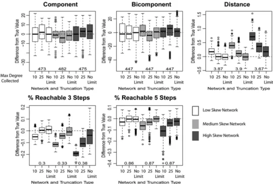
6.1. Results Part 1: Researcher Does Nothing in Response to Degree Truncation Figure 5 presents a snapshot view of the results. The figure is organized by global mea-sure of interest. There is a separate set of boxplots for component size, bicomponent size, distance, three-step reachability, and five-step reachability. The x-axis in each subplot cor-responds to truncation level, moving from strong truncation (at 10) to medium truncation (at 25) to no truncation. Each boxplot captures the difference between the true values and the estimates taken from the simulation. The boxplot values are positive if the simulation overestimates the true value. The boxplots are also divided by network of interest, ranging from low skew to high skew. Boxplots corresponding to the same network have the same color (e.g., white = low skew). I have placed the true value for each network/measure un-derneath the boxplots as a point of reference. The estimates for each network/truncation level are good if they are centered around 0 and have low variance.
I begin with component and bicomponent size. Here the results are encouraging. The method successfully produces good estimates, and this is true for every network and every level of truncation. It is not the case, as we might expect, that the estimates deteriorate as truncation increases. It is even possible to estimate the size of the larg-est component and bicomponent when the network is highly skewed and degree is truncated at 10. Thus, a researcher interested in component or bicomponent size could make inference using sampled data even under particularly difficult conditions. (Note
18 Although it is important to note that under no truncation the researcher response is not varied, as there is nothing to try and “fill in.”
that there are also analytical solutions showing if there is a giant component in the net-work; Grannis, 2010.)
The distance results are more heterogeneous, dependent on both the level of skew in the network and the level of truncation in the survey. Beginning with the low skew (white) net-work, there is little bias under no truncation and medium truncation (close to no trunca-tion for the low skew network). There is, however, some bias when the survey is strongly truncated, allowing only 10 alters to be named. Thus, as long as degree is not strongly trun-cated, it is possible to produce accurate estimates for distance on the low skew network. Even when the survey is strongly truncated, the bias is under 5%. The medium skew net-work offers a similar story, with severe bias only when the degree distribution is truncated at 10, and essentially no bias with no truncation. We begin to see systematic bias in the high skew network. The true distance is 3.67 while the mean estimate is 4.40 under strong trun-cation (see Table A3 in the Appendix). The bias clearly decreases as the level of truntrun-cation decreases: The mean estimate is 4.01 when truncating at 25 and 3.84 with no truncation. Yet there is still residual bias even when the researcher has full information on the sample. Under no truncation, the interquartile range (IQR) is (3.67, 4.03), just barely including the true value. Figure A1 in the Appendix presents the full distance distribution. The method once again reproduces the true distance between nodes when there is no truncation, but overestimates distance under strong truncation. For example, in the medium skew network under strong truncation, the simulated networks underestimate the number of nodes that are separated by two or three paths and overestimate the number separated by four or five paths—but this is not the case when there is no or weak truncation in the survey.
Reachability offers similar results. There is noticeable bias for the low skew network only when the survey is strongly truncated (limited to 10 alters); the high skew net-work, in contrast, has some bias and large variance even when there is no limit on the number of alters a respondent can name. Similarly, there is little bias in the medium skew network when there is no truncation but significant bias when the survey is trun-cated at 10. The method generally underestimates the true value. For example, the true value in the medium skew network is .327 while the mean estimate is .286 (under me-dium truncation).
Five-step reachability yields much lower bias than three-step reachability and is easier to estimate on the whole. It is even possible to estimate five-step reachability on the high and medium skew networks, as long as the survey is not truncated at 10. The low skew net-work is estimated quite well at all levels of truncation.
In short, it is clear that some measures/networks are easier to estimate than others (e.g., bicomponent size versus distance; low skew versus high skew networks) while truncated surveys lead to worse estimates. Encouragingly, a researcher can accurately estimate many global measures even if they do nothing in response to survey limitations (i.e., the low and medium skew networks when the survey is not strongly truncated).
6.2. Results Part 2: Filling in the Truncated Degree Distribution
Figure 6 presents the results for the imputed tail analysis. The figure has the same form as Figure 5, but now the researcher imputes the truncated portion of the degree distribution. Figure 6. Estimates for global measures by network and truncation type: Simulate truncated tails.
As before, the method produces excellent estimates for component and bicomponent size across all networks and survey designs.
The results for distance are quite different than in Figure 5, where there was no response from the researcher. Here, there is no bias when estimating distance in the low skew net-work, even when the survey is truncated at 10. The bias is also reduced in the medium skew network, although there is still some bias under strong truncation. The results for the high skew network show little improvement, however. The full distance distribution (see Fig-ure A2 in the Appendix) offers an analogous story. There is only bias for the medium skew network under strong truncation (again, underestimating the number of shorter paths in the network), and none for the low skew network.
The results are similar for three-step reachability: there is no bias for the low skew net-work across all survey designs, while the medium skew netnet-work shows lower bias than before (for both strong and medium truncation). The five-step reachability results are very similar across the no response and imputed tails figures.
Overall, filling in the degree distribution improves the estimates in every case but the high skew network. It is now possible to estimate the medium skew network for all survey designs expect the strong truncation case, while there is no bias for the low skew network, independent of survey design.
6.3. Results Part 3: Using Categorical Responses
Figure 7 presents the results for the categorical response analysis. Here, the researcher asks the respondents to estimate their number of alters (if above the truncated number); they then use that information to fill in the truncated portion of the degree distribution. Figure 7. Estimates for global measures by network and truncation type: Use categorical responses.
Once again, component size and bicomponent size are accurately estimated for all net-works and survey designs. The distance results, however, largely favor the categorical re-sponse approach—both compared with doing nothing and imputing the tails of the distri-bution (although this does not hold for the medium skew network at medium truncation). Using categorical responses, one can accurately estimate distance for the low skew and me-dium skew networks under any level of truncation. Similarly, the bias for the high skew network is much reduced under the categorical response approach. For example, the true distance in the high skew network is 3.67; the IQR is (3.91, 4.10) when imputing the tails and (3.61, 4.07) when using categorical responses (under medium truncation). The story is similar for three-step reachability. It is possible to estimate reachability well for the me-dium skew network at all levels of truncation, although the best estimates still come when there is no truncation. There is essentially no bias for five-step reachability, and this holds for all networks and all truncation levels.
Tables A1–A5 in the Appendix focus more explicitly on the role of the researcher. The tables are organized around measures, with one table per global statistic of interest. Within the tables, the columns correspond to different researcher responses: no researcher response; impute truncated tails; use categorical responses. The rows capture the level of skew in the network and the level of truncation in the survey.
Beginning with distance (Table A3 in the Appendix), it is clear that the categorical re-sponse approach offers the lowest bias when there is strong truncation (at 10) and the net-work has medium or high skew. For example, the true distance score in the medium skew network is 3.90. Under strong truncation, the mean estimate is 4.29 when doing nothing, 4.15 when imputing the tails, and 4.00 when using categorical responses. This general pat-tern also holds for reachability. There is thus good reason to use categorical responses when the survey has a strongly truncated degree design. Similarly, the high skew network is al-most uniformly handled best by the categorical response approach.
It is not the case, however, that categorical responses will always offer the best option. For example, in the medium skew network under medium truncation (truncated at 25), fill-ing out the degree distribution is generally preferable to usfill-ing categorical responses. Simi-larly, the low skew network is handled equally well by both approaches (and both are bet-ter than doing nothing). In general, the categorical response approach is most appropriate when the information about the network is limited: so that truncation is strong or the skew of the network is high. Either active approach (i.e., imputing the tails or using categorical responses) is better than doing nothing, which is only appropriate when the network is not skewed and there is no survey truncation.
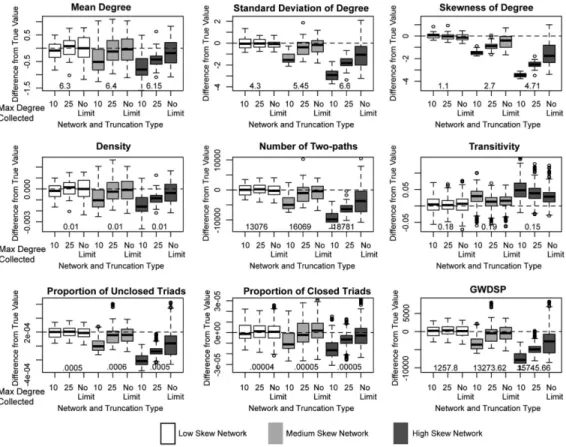
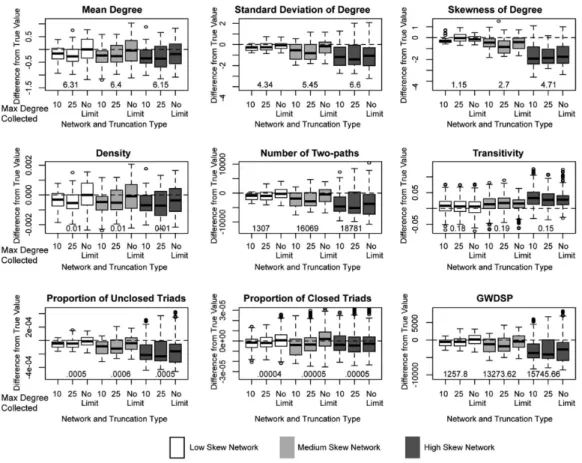
7. Results: Local Network Measures
The global network results are encouraging, but it is important to see if the same trends hold for the local measures. Collectively, the local measures capture: (a) the properties of the degree distribution (or the number of ties per person), (b) the level of local closure (is a friend of a friend a friend?), and (c) the level of higher order clustering (i.e., how many
friends does i and j have in common?). Measures of cohesion and connectivity exhibit a reg-ularity that the local measures often lack (as they are more robust to small changes), mak-ing this a more difficult test of the method.
Figures 8 to 10 present the results for the local network measures (see also Tables A6– A13 in the Appendix.) The top line of Figures 8 to 10 presents the results for the mean, stan-dard deviation and skew of the degree distribution. It is clear from the figure that mean degree is accurately estimated in the low and medium skew networks when there is no truncation. The estimates for mean degree are only slightly biased downwards when trun-cation is weak (truncated at 25). Under strong truntrun-cation, it is important for the researcher to take some action. For example, for the low skew network, under strong truncation, the mean bias is about 3% under the actual value based on categorical responses but 10% if the researcher does nothing. The results are similar for the high skew network, although the bias is higher at every level of truncation. Note that the density plot is a scaled version of the mean degree plot, and offers identical results.
The bias is higher for the standard deviation and skew of the degree distribution: there is little bias in the low and medium skew networks under no truncation, but some bias when the survey is truncated, even when imputing the tails or using categorical responses. The bias is particularly noticeable for the medium skew network. It is even harder to estimate Figure 8. Estimates for local measures by network and truncation type: No researcher response.
the skew and standard deviation in the high skew network. This is true at all levels of trun-cation and for all researcher responses (although categorical responses fares the best of the three). For example, the bias in standard deviation is upwards of 25% under weak trun-cation. The results suggests three things: first, that the sample is missing the high degree nodes in the high skew network; second, that the method is underestimating the degree of the truncated cases in the medium skew network; and third, that the high degree nodes have a large impact on the shape of the degree distribution.
The remaining measures capture local clustering and reachability in the network. The first measure, number of two-paths, is estimated quite well in the low skew net-work, especially when simulating the tails of the distribution (with bias under 1%). The worst estimate is the case of strong survey truncation and no researcher response. Similarly, the medium skew network is estimated well under weak truncation (when simulating the tails of the distribution) and no truncation (bias under 5%). The largest bias clearly resides with the high skew network, where the number of two-paths is underestimated across the board. This is the case as high degree nodes create many two-paths; missing those high de-gree nodes means underestimating the extent of local reachability.
In a similar manner, the proportion of unclosed triads is estimated well in the low and medium skew networks and underestimated in the high skew network. For example, in the
low skew network, the bias under no truncation is 2%. The closed triad estimates are even better, with little bias for the low and medium skew networks under weak or no truncation. Under strong truncation, the estimates are still quite good for the low skew network, save in the case of no researcher response. The bias is also much lower for the high skew net-work; under no truncation, the bias is 5% for closed triads but 20% for unclosed triads. The unclosed triads are more sensitive to missing high degree nodes because high degree nodes often connect people who are themselves not connected (just as we saw with two-paths).
The final plot presents the results for the geometrically weighted dyad shared partner distribution. The measure captures higher-order clustering in the network, or the tendency for individuals to have more than one friend in common. The high skew network, once again, offers the worst estimates, with bias of 16% under no truncation. The method per-forms quite well otherwise, even though ego network data do not directly capture these wider connections. There is very little bias for the low skew network, and this holds for all levels of truncation (under categorical responses or simulating tails). Similarly, the method estimates GWDSP well for the medium skew network under no truncation. Under strong truncation, the categorical response approach performs best, with bias around 11%; under weak truncation, simulating the tails performs best, with bias around 5%.
8. Conclusions
Network sampling holds great promise for network scholars and public policy practitio-ners. The benefits of sampling are clear: a researcher no longer needs a census to analyze the network structure of a system (Handcock & Gile, 2010). Network sampling can be quite difficult, however, and we are still trying to understand when accurate inference is possi-ble and when it is not (Smith & Moody, 2013). Ego network data pose an extreme example of the network sampling tradeoff. Ego network data are easy to collect for the very reason inference is hard: the sample only collects bits of information about the respondents and their social connections. The question is how far one can push ego network data and simu-lation techniques in making inference about global network properties—such as cohesion, diffusion potential or group structure.
Past work has demonstrated the validity of simulation techniques on a restricted range of networks. The simulation approach of Smith (2012) yields accurate estimates for net-works without a skewed degree distribution and surveys that do not truncate (or limit) the number of alters named. The test here explored a wider range of circumstances: I systematically varied the level of degree skew in the network and the level of truncation in the survey when evaluating the method. I also asked if the researcher could limit the level of bias.
The low skew network represents the case closest to previous tests. Here, the top-de-gree node has less than 25 ties. Low skew networks characterize many networks of inter-est, including networks based on close friendship, confidants, and social support (Well-man & Wortley, 1990; Smith et al., 2014). The results suggest that one can accurately make global network inference in low skew networks under all survey conditions. The researcher must, however, treat the data in some way (using categorical responses or im-puting the tails) when the survey is strongly truncated. Similarly, there is little bias for the local clustering measures. This holds for all truncation levels, as long as the researcher does something to deal with the truncation in the survey (with imputing the tails offer-ing the better option).
The results for the medium skew network are similarly encouraging. The medium skew network has a high degree around 50, representing networks of weak friendship or regu-lar affiliation (Moody, 2004). The model produces accurate global network estimates when there is no degree truncation. When there is degree truncation, the results clearly depend on the response of the researcher. The categorical response approach offers accurate esti-mates across all survey designs, while imputation is a viable option for all but the strongest level of truncation. It is, however, quite difficult to produce unbiased estimates when the researcher does nothing in response to survey truncation (although one can still estimate component and bicomponent size without bias). The method also performs well for more local network measures, although the bias is generally higher than with the global mea-sures. The method is particularly appropriate for local clustering measures when there is no/weak truncation, but less appropriate if the survey is strongly truncated.
Taken together, simulation based inference is appropriate for many empirical settings of interest—ranging from the close ties of friendship and cohabitation to the wider ties of regular affiliation and association.