Determinants Of Foreign Direct Investment Inflows In
Swaziland’s Agricultural Sector
M.S. Dlamini1, M.B. Masuku2 and M.O. Raufu2 1
P.O.BOX 986 Manzini, Swaziland 2
Faculty of Agriculture and Consumer Sciences, University of Swaziland, P.O. Luyengo, Swaziland.
ABSTRACT
Foreign direct investment plays a significant role in the development and growth of developing countries. The main objective of the study was to analyse the determinants of foreign direct investment inflows in Swaziland’s agricultural sector from 1990 to 2014. The study examined the long-run and short-run effects by using the cointegration th
eory and the error correction model. The dependent variable was agriculture foreign direct investment inflows stock, while the explanatory variables were; government foreign debt, nominal GDP, trade openness, exchange rate, inflation and investment promotion. The study used the Breusch-Pagan-Godfrey test for heteroscedasticity. The Engle-Granger cointegration test was conducted to test the hypothesis that there was no cointegration between the dependent variable and the independent variables. The long-run regression results revealed that nominal GDP and investment promotion were positive and significant determinants of agriculture FDI (p<0.01). Their coefficients were 1.393 and 0.983 respectively. In the short-run, trade openness and investment promotion were significant and positive (p<0.01) with coefficients of 1.483 and 1.05 respectively. The error correction model was within the acceptable range and it had the expected negative sign. Its coefficient was -0.431 suggesting that about 43% of the short-run shocks were adjusted back to the long-run path within a year. The study recommends that the Swaziland Government must focus on increasing the rate of GDP growth mainly through the encouragement of processing of raw materials to finished goods and also improve on openness to trade.
Keywords: Agricultural foreign direct investment, cointegration model, trade openness, nominal GDP. 1. INTRODUCTION
1.1 Background
Swaziland is a developing country with a small economy and a real GDP growth rate of 2.8 percent in 2013. It is classified as a lower-middle-income country with a GDP per capita of US$2,548 (2013/2014). The average inflation rate is currently estimated at 6.2% (Central Statistics Office, 2015). Swaziland is a member of the Southern African Customs Union (SACU) and Common Market for Eastern and Southern Africa (COMESA). Its main trading partners are South Africa, European Union and the United States of America (USA). With the USA it has trade preferences under the African Growth and Opportunity Act, AGOA, which is currently suspended from benefiting because it has to meet required some benchmarks. Swaziland’s currency, Lilangeni is pegged to the South African Rand. The country’s economy is diversified with agriculture, forestry and mining accounting for about 13% of GDP. The manufacturing sector (textile and sugar-related processing) accounts for 37% of GDP and services constituting 50% (UNCTAD, 2014).
Swaziland’s economic growth has lagged behind compared to those of its neighbours. Real GDP growth since 2001 has averaged at 2.8%, nearly 2% points lower than the growth in the other SACU member countries. Low agricultural productivity in SNLs, repeated droughts, the devastating effect of HIV and AIDS and an overly large and inefficient government sector are possible contributors. The country’s public finances deteriorated in the late 1990s following sizeable surpluses in the early 90’s. During this time, a combination of declining revenues and increased spending led to significant budget deficits (UNCTAD, 2014). According to the Central Bank of Swaziland (2013), the Swazi economy is very closely linked to the South African economy with over 90% of its imports coming from South Africa. Swaziland sends about 70% of its exports to South Africa. The country is faced with challenges in trying to improve the investment climate which include poor governance issues. However it is trying to lure foreign direct investment through the Swaziland Investment Promotion Authority (SIPA).
The inflows of FDIs are extremely important in Swaziland’s economy due to shortage of savings, investment capital and deficiency of capital for developmental projects. The foreign capital is important for the country’s economy in terms of the growth of industries, reduction of unemployment and technological improvements, which may eventually result in economic development and growth. The agricultural sector in Swaziland is one of the most important sectors as it provides employment opportunities to thousands of people and contributes significantly to GDP (IMF, 2013). This sector is expected to fulfill local demand for food items and increase exports of different agricultural commodities to foreign countries.
The economy of Swaziland has attracted total inflows of FDI amounting to US$673 million in 2013, which shows a decrease from the previous year, which was US$678 million. The inflows of FDI within the agricultural sector amounted to US$88 million in 2011, US$149 million in 2012 and US$96.5 million in 2013 (Central Bank of Swaziland, 2014). The FDI in the agricultural sector is still not sufficient as it even shows some fluctuations. 1.2 Statement of the Problem
According to IMF (2013), inspite of Swaziland’s middle-income status, it is characterised by high levels of inequality, high poverty rate which was 63% of the population in 2010, food insecurity which was 29% of population in 2010 and unemployment which was 29% of the labour force in 2010. The uneven income distribution stems from low job creation and the absence of adequate social protection. Swaziland’s economy is also agricultural based thus the extent to which FDI can help reduce these challenges depend on the amount of the FDI inflows into this sector. According to Djokoto (2012), FDI in the agricultural sector is likely to employ unskilled labour and provide benefits to the rural areas in that way reducing poverty to the people living there. With increased FDIs, there will be increased land productivity which is currently rated very low. This will be as a result of the technology that comes with FDIs.
However, with the high level of poverty and unemployment in Swaziland, there are low savings and investment especially in the agricultural sector and there is a need for the country to get sufficient FDI inflows in order to close the gap between saving and investment. The FDI inflows into the agricultural sector are fluctuating and insufficient thus this gap is difficult to close. Although the country has improved in the ease of doing business, investors may still consider investing in other countries that are ranked at the top of Swaziland in terms of indicators like starting a business, getting electricity and protecting investors (Times of Swaziland, 07,
November 2014). Therefore identifying the determinants of inward FDI into the agricultural sector will provide useful information especially to policy makers for them to draft new policies which will ensure sufficient supply of FDI into the agricultural sector in Swaziland.
1.3 Objectives of the study
The main objective of the study is to examine the determinants of agriculture FDI inflows in Swaziland. Specifically the objectives are;
(i) To analyse the economic determinants of agriculture FDI inflows in Swaziland, (ii) To identify policy initiatives aimed at improving agriculture FDI inflows in Swaziland
2. THEORETICAL FRAMEWORK
Theories of FDI can be split into two levels, namely micro-level determinants of FDI and macro-level
determinants of FDI. The micro-level theories of determinants of FDI give reasons why multinational companies (MNCs) prefer opening subsidiaries in foreign countries as compared to exporting or licensing their products. It also explains how MNCs choose their investment locations and why they invest where they do. The macro-level determinants deal with the host countries situations that determine the inflow of FDI.
2.1 Micro-level Theories of FDI
2.1.1 The Early Neoclassical and Portfolio Investment Approaches
According to the early neoclassical approach, interest rate differentials are the main reason for firms to become multinational companies. Capital moves from a country where return on capital is low to a place where return on capital is high and vice versa. This approach is based on perfect competition and capital movement free of risk assumptions (Harrison et al, 2000). However, the movement of capital is not unidirectional.
2.1.2 The Product Life Cycle Theory of FDI
According to Dunning (1993), a new product is first produced and sold in the home market. At the early stage, the product is not standardized, i.e. the per unit costs and final specification of the product are not uniform. As the demand for the product increases the product will be standardized. When the home market is saturated, the product will be exported to other countries. The firm starts to open subsidiaries in locations where the cost of production is lower, when the competition from the rival firms intense and the product reaches its maturity. Therefore, FDI is the stages in the product lifecycle that follows the maturity stage (Dunning, 1993). 2.1.3 Internalization Theory of FDI
Krugman and Obstfeld (2003) suggested that in order to increase profitability, some transactions should be carried out within a firm rather than between firms and this is one of the reasons why multinational companies exist. In other words, there are transactions that should be internalized to reduce transaction costs and hence increase profitability. This theory may answer the question on why production is carried out by the same firm in different locations. One of the reasons of internalization is market imperfection. Any kind of economically useful knowledge can be called technology. Mostly, technologies or knowhow can be sold and licensed. However, sometimes there are technologies that are embodied in the mind of a group of individuals and not possible to write or sell to other parties, (Krugman & Obstfeld, 2003). This difficulty of marketing and pricing know-how forces MNCs to open a subsidiary in a foreign country instead of selling the technology. In addition, a number of problems may arise if an output of a firm is an input to other firm in other country. For instance, if each has a monopoly position, they may get into a conflict as the buyer of the input tries to hold the price down while the firm that produces input tries to raise it. Nevertheless, these problems can be avoided by integrating various activities within a firm rather than subcontracting the activities, (Krugman & Obstfeld, 2003).
2.1.4 The Eclectic Theory of FDI
The FDI theory according to Dunning (1993) which is known as Dunning’s Eclectic paradigm, states that the extent, geography and industrial composition of foreign production undertaken by multinational enterprises is determined by the interaction of three sets of interdependent variables. They themselves comprise the components of three sub units, (Dunning, 2001). Mathematically this can be represented as;
FDI = ƒ(O, L, I), where O is ownership, L is location and I is internalization.
According to Dunning (2001), these three variables are key competitive advantages in this theory. The
ownership competitive advantage theorizes that at ceteris paribus, the greater the competitive advantages of the investing firms relative to those of other firms, the more they are likely to be able to engage in foreign
production. The locational attractions postulates that the more the immobile, natural or created endowments needed by the firm to jointly use with their own competitive advantages, favor a presence in a foreign location, the more firms will choose to supplement or take advantage of their ownership specific advantages by engaging in FDI. The last competitive advantage is internalization. This offers a framework for evaluating alternative ways in which firms may organize the creation and exploitation of their core competences, given the locational attractions of different countries or regions.
2.2 Macro-level Determinants of FDI
The macro-level determinants of FDI include any host country’s situations that affects the inflow of FDI, like market size, the economic growth rate, GDP, infrastructure, natural resource, and the political situation. 3. METHODOLOGY
3.1 Research design
A descriptive research design with time series data from 1990 to 2014 was used. Total gross annual agricultural FDI inflow as defined by UNCTAD was used as the dependent variable. Annual real GDP, annual exchange rate, annual inflation rate, agricultural trade openness calculated as a ratio of exports and imports to GDP, investment promotion and a dummy were used as the independent variables.
3.2 Data Sources
The data were obtained from the Central Bank of Swaziland. For the last variable, government foreign debt, data were obtained from the Central Statistics Office. The period for the study is from 1990 to 2014.
3.3 Data analysis
The main objective of the study was to analyze the determinants of agriculture foreign direct investment inflows in Swaziland. In order to achieve this, the error correction model (ECM) was used and the analysis was
conducted using Econometric Views (E-Views) 5 software. 3.3.1 Model Specification
From the literature and theoretical framework developed, the following model was adopted for the first objective of this study. The model includes the determinants of FDI as independent variables. Therefore the function is; AgFDI = f (NGDP, ER, AGTOP, INF, IP, GDT)
Where
AgFDI = inflow of agriculture foreign direct investment. The size of this variable is a good indicator of the relative attractiveness of an economy to agriculture foreign investment. It is also a vehicle for the economic growth of developing countries.
NGDP = is the nominal gross domestic product. It measures the size of the home economy and it is included in order to control for the supply of FDI. The assumption is that growth in the host country is likely to generate a greater supply of FDI. For this study, a positive relationship between RGDP and AgFDI is expected.
ER = exchange rate. This measures the worth of the domestic currency in terms of another currency. It is necessary in order to show how the strength of a nation’s currency affects her inward FDI. The expected sign of the exchange rate with respect to AgFDI is negative.
AGTOP = agriculture trade openness. Romer (1990) constructed an openness measure based on geographical characteristics. The revealed openness measure is the most commonly used in most empirical studies. It is clearly defined, well measured and available for most countries. In this study, the revealed openness or the ratio of imports and exports to GDP is used as a measure of openness in this study. Greater openness is expected to have a positive effect on FDI inflows.
INF = this is the inflation rate. According to Lim (2001), low inflation is taken to be a sign of internal economic stability in the host country. Any form of instability introduces a form of uncertainty that distort investor perception of the future profitability in the country. A stable economy attracts more FDI thus a low inflation environment is desired in countries that promote FDI as a source of capital flow. Therefore we expect a negative relationship in the regression analysis.
IP = investment promotion. If a country promotes itself, we expect more foreign direct investment inflows. Thus a positive relationship is expected with the dependent variable.
GDT = government foreign debt. Excessive foreign debt is one source of instability and uncertainty in
macroeconomic environment of underdeveloped countries and hence it is likely to affect adversely the inflow of FDI. Excessive foreign debt may signal imminent fiscal crises and foreshadow the future economic situation in a county (Serven and Solimano, 1992). A negative relationship is expected between this variable and the
dependent variable.
The statistical form of the model is:
AgFDIt = β0 + β1NGDPt + β2ERt + β3AGTOP +β4INFt + β5IP + β6GDT + µt
Where βi is the parameter estimate of the independent variables and µt being the random variable or the error term.
The independent variables were all lagged by one year to capture the effect that these variables have on the current year’s foreign direct investment inflows. Also these variables were converted into logarithms for the easy interpretation of the coefficients as elasticity coefficients. However, inflation was not logged because it is in percentage form. Also the dummy investment promotion was also not lagged because we used zero before SIPA was established. Thus the model was specified as:
lnAgFDIt = β0 + β1lnNGDPt + β2lnERt + β3lnAGTOP +β4INFt + β5IP + β6lnGDT + µt
Where; AgFDI is annual agriculture FDI inflows in Swaziland, NGDP is annual nominal GDP
ER is the annual nominal exchange rate, AGTOP is trade openness which is a ratio of agricultural exports and imports to GDP, INF is the annual average inflation rate, IP is the level of investment promotion. A dummy variable was used. Since SIPA was established in 1998, then from 1998 to date, the dummy was one and the period from 1990 to 1998 was zero and GDT is government foreign debt.
To test for heteroscedacity, the study used the Breusch-Pagan-Godfrey test which tests the null hypothesis that the residuals are homoscedastic against the alternative that the residuals are heteroscedastic. To detect whether the residuals are normally distributed or not, the study used the Jarque–Bera Statistic.
The error correction model (ECM) was used in the study. Before the ECM is estimated, all the variables were tested for unit roots. In other words, the ECM is to be subjected to the random walk hypothesis, with the mean value being zero and constant standard deviation.
4. RESULTS AND DISCUSSION 4.1 Testing for Heteroscedasticity
To test for heteroscedacticity, the study used the Breusch-Pagan-Godfrey test which tests the null hypothesis that the residuals are homoscedastic against the alternative that the residuals are heteroscedastic. If the p-value of the Chi-square (χ2) is less than 0.05 (p < 0.05), the null hypothesis of homoscedasticity is rejected in favour of the alternative. After conducting this test, the results showed that the model does not suffer from a problem of heteroscedasticity. The p-value of the F-statistic was 0.463 which is greater than 0.05.
4.2 Testing for Normality
One of the main assumptions of the classical normal linear regression model is that the residuals are normally distributed. The hypothesis tests on the coefficients obtained by OLs are based on this assumption. To detect whether the residuals are normally distributed or not, the study used the Jarque –Bera Statistic. The null
hypothesis is that the residuals are normally distributed against the alternative that the residuals are not normally distributed. Again if the p-value of Jarque-Bera statistics is less than 5 percent (0.05) we reject null hypothesis that the residuals are normally distributed and accept the alternative, that is, residuals are not normally distributed.
4.3 Stationarity and integration test results
In order to avoid spurious regressions, stationarity tests were the pre-tests that had to be done. For a
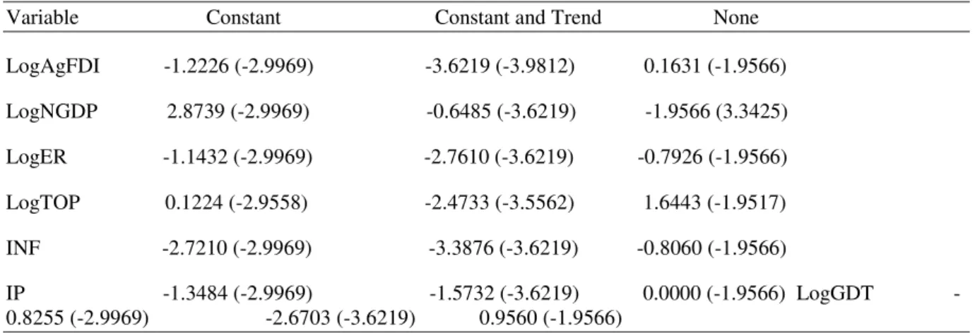
non-stationary series, the order of integration is determined by the number of times it has to be differenced in order to attain stationarity. In this study, the Augmented Dickey-Fuller test was used to test for the unit roots. All the time series variables in the equation were tested for unit roots. The test results demonstrated that all the variables cannot reject the hypothesis of unit roots I(O). This means that the variables were all non-stationary. The variables were non-stationary because their ADF statistics were smaller than the Mackinnon critical values for rejection of the hypothesis for unit roots as shown in Table 1.
Table 1 ADF results before differencing non-stationary variables.
Variable Constant Constant and Trend None LogAgFDI -1.2226 (-2.9969) -3.6219 (-3.9812) 0.1631 (-1.9566) LogNGDP 2.8739 (-2.9969) -0.6485 (-3.6219) -1.9566 (3.3425) LogER -1.1432 (-2.9969) -2.7610 (-3.6219) -0.7926 (-1.9566) LogTOP 0.1224 (-2.9558) -2.4733 (-3.5562) 1.6443 (-1.9517) INF -2.7210 (-2.9969) -3.3876 (-3.6219) -0.8060 (-1.9566) IP 1.3484 (2.9969) 1.5732 (3.6219) 0.0000 (1.9566) LogGDT -0.8255 (-2.9969) -2.6703 (-3.6219) 0.9560 (-1.9566)
Note: Numbers in brackets are Mackinnon critical values at 5% level of significance.
After the variables were differenced once, the test results show that all the variables were stationary thus the hypothesis of unit roots I(1) was rejected. The results are presented in Table 2.
Table 2 ADF results after differencing non-stationary variables once.
Variable Constant Constant and Trend None
∆LogAgFDI -6.1382 (-3.0038) -5.9642 (-3.6330) -5.7295 (-1.9574) ∆LogNGDP -4.2462 (-3.0114) -4.1305 (-3.6454) -4.1931 (-1.9583) ∆LogER -3.3871 (-3.0038) -3.6402 (-3.6330) -2.7564 (-1.9574) ∆LogTOP -3.1377 (-3.0114) -3.7337 (-3.6454) -3.2265 (-1.9583) ∆INF -4.824 (-3.0038) -4.7163 (-3.6330) -4.8908 (-1.9574) ∆IP -3.3166 (-3.0038) -3.6453 (-3.6330) -3.1623 (-1.9574) ∆LogGDT -5.2321 (-3.0114) -5.0808 (-3.6454) -5.3759 (-1.9585)
Note: Numbers in brackets are Mackinnon critical values at 5% level of significance. ∆ denotes that the variable was differenced once.
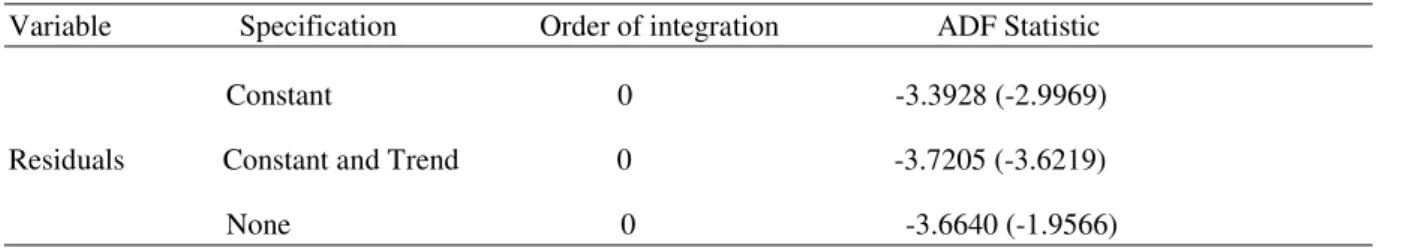
4.3 Cointegration test results
Since the variables are cointegrated of order one I(1), then we have to test for cointegration amongst the variables. This helps in establishing if the linear relationship of the variables is stationary. If the linear combination of the variables is stationary, that means the null hypothesis of no cointegration is rejected thus a spurious log-run relationship exists between the variables and as such consistent estimates of the long-run elasticities will be evident (Xinzhong, 2005).
Table 4.3 Cointegration test results
Variable Specification Order of integration ADF Statistic Constant 0 -3.3928 (-2.9969) Residuals Constant and Trend 0 -3.7205 (-3.6219) None 0 -3.6640 (-1.9566) Note: Numbers in brackets are Mackinnon critical values at 5% level of significance.
The results in Table 4.3 indicate that there is cointegration amongst the variables. This means that the null hypothesis of no cointegration is rejected. The residuals from the regression are stationary I(0). This is because the Mackinnon critical values are smaller than the ADF statistic. In a case like this where cointegration has been confirmed amongst the variables, then the cointegration relationship and dynamic relationship which
incorporates the equilibrium and how the short-run adjustments to that equilibrium are made (Masuku & Dlamini, 2009).
4.4 The Error Correction Model Results
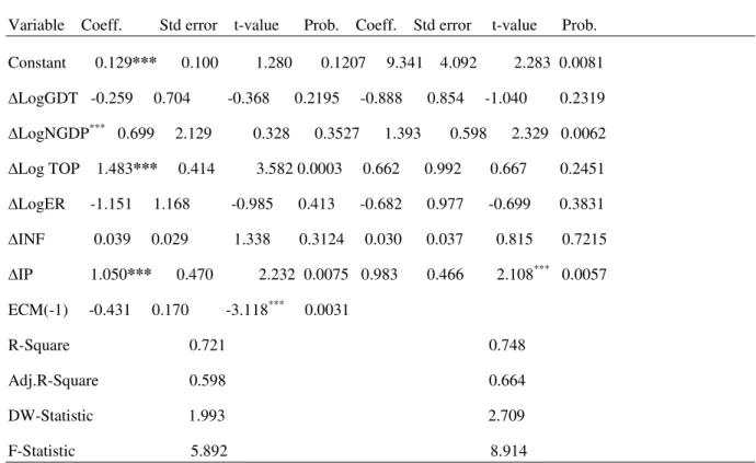
The results shown in Table 4 below indicate that the signs of the coefficients in both the short-run and lon-run models are the same. The signs for all the variables were found to conform to our prior expectation. The variables government foreign debt (GDT), exchange rate (ER) and inflation rate (INF) had negative signs in the short-run. This means that a decrease in each of the variables results in an increase in agriculture foreign direct investment inflows (AgFDI). On the other hand, the variables nominal GDP (NGDP), trade openness (TOP) and investment promotion (IP) had positive signs implying that a unit increase in each one of them results in an increase in agriculture foreign direct investment inflows.
The variables in the short-run model explain about 72% of the variation in agriculture FDI inflows stock. In the long-run, the variables explain about 75% of the variation in agriculture FDI inflows stock. The value of Durbin Watson statistics is 1.993, which indicates that there is no problem of multi-collinearity as the value is within acceptable range of 1.5-2.5. The response of the variable government foreign debt is negatively related to agriculture FDI inflows. The coefficient was -0.259. This means that a 10% increase in government foreign debt results in a decrease in agriculture FDI inflows by 0.259%. However this variable was insignificant.
The nominal GDP had a positive relationship with the dependent variable with a coefficient of 0.699. This implies that in the short-run, a 10% increase in the nominal GDP results to agriculture FDI inflows increase by 0.699%. The trade openness also had a positive relationship with the dependent variable with a coefficient of 1.483. This means that a 10% increase in trade openness results to an increase of 1.483% in agriculture FDI inflows. Djokoto (2012) and Zeshan et al (2013) both found the same positive relationship and both variables were significant in their respective studies. However in this study nominal GDP was insignificant whilst trade openness was (P<0.1).
The exchange rate showed a negative relationship with a coefficient of -1.151 in the short-run model. This means that a 10% increase in the exchange rate will reduce agriculture FDI inflows by 1.151%. The inflation rate and investment promotion both had positive relationships with the dependent variable. The coefficient for inflation rate in the short-run was 0.039 meaning that a 10% increase in the inflation results to a 0.039% increase in agriculture FDI inflows. However such is not new as Zeshan etal (2013) also found the same, but Djokoto (2012) found it to be negative. The coefficient for investment promotion was 1.0502 in the short-run implying that a unit increase in investment promotion increases agriculture FDI inflows by 1.05%.
Table 4 The Error Correction Model Results Dependent Variable: ∆LogAgFDI
Short-Run Long-Run Variable Coeff. Std error t-value Prob. Coeff. Std error t-value Prob. Constant 0.129*** 0.100 1.280 0.1207 9.341 4.092 2.283 0.0081 ∆LogGDT -0.259 0.704 -0.368 0.2195 -0.888 0.854 -1.040 0.2319 ∆LogNGDP*** 0.699 2.129 0.328 0.3527 1.393 0.598 2.329 0.0062 ∆Log TOP 1.483*** 0.414 3.582 0.0003 0.662 0.992 0.667 0.2451 ∆LogER -1.151 1.168 -0.985 0.413 -0.682 0.977 -0.699 0.3831 ∆INF 0.039 0.029 1.338 0.3124 0.030 0.037 0.815 0.7215 ∆IP 1.050*** 0.470 2.232 0.0075 0.983 0.466 2.108*** 0.0057 ECM(-1) -0.431 0.170 -3.118*** 0.0031 R-Square 0.721 0.748 Adj.R-Square 0.598 0.664 DW-Statistic 1.993 2.709 F-Statistic 5.892 8.914
Note: ∆ denotes that variables were differenced once to attain stationarity. *, ** and *** indicate significance levels at 10%, 5% and 1% respectively.
The results of the error correction model (ECM) or residuals in the short-run give the percentage of the deviation from the long-run equilibrium which is eliminated yearly. The coeffiecient was -0.431. This implies that about 43% of the deviation of agriculture foreign direct investment inflows stock from the equilibrium mean is eliminated annually in this relationship.
In the long-run the signs of the coefficients are the same as in the short-run analysis. Nominal GDP had a positive and significant relationship with the dependent variable with a coefficient of 1.393. This means that a 10% increase in nominal GDP results to a1.393% increase in agriculture FDI inflows. Investment promotion showed a positive and statistically significant relationship with the dependent variable, agriculture FDI. Its coefficient is 0.983 which implies that a 10% increase in investment promotion results to a 0.983% increase in agriculture FDI inflows. The other variables, government foreign debt, trade openness, exchange rate and inflation were all insignificant.
5. CONCLUSIONS AND RECOMMENDATIONS 5.1 Conclusions
Foreign direct investment plays a significant role in the development and growth of developing countries. This study was done to identify the factors that determine foreign direct investment inflows in Swaziland’s
agricultural sector. From the results, it can be concluded that trade openness and investment promotion induces agriculture foreign direct investment inflows in Swaziland in the short-run while nominal GDP and investment promotion induce agriculture foreign direct investment inflows in Swaziland in the long-run. The other variables, government foreign debt, exchange rate and inflation do not attract agriculture foreign direct investment in Swaziland both in the short -run and long-run.
In the analysis, the error-correction model (ECM1 -1) was found to be significant at one percent and had a negative coefficient of -0.431 suggesting that any short-run deviation of agriculture foreign direct investment inflows adjusts to its determinants with a lag and that only about 43% of the discrepancy between the long run and short run agriculture foreign direct investment inflows is corrected within a year and it was in accordance with our prior expectation of the ECM which is supposed to be negative and less than one. From the hypotheses it can be concluded that in the long-run, the null hypothesis cannot be rejected for nominal GDP and trade openness, but for the other variables the alternative hypothesis is accepted. In the short-run the null hypothesis cannot be rejected for the variables trade openness and investment promotion and for the other variables the alternative hypothesis is accepted.
5.2 Recommendations
In the light of the above discussions and conclusions the growth rate of the economy of the country should be increased to increase FDI inflows into the agricultural sector. Also, the country needs to further improve its trade openness as it was found to be one of the factors that determined agriculture FDI inflows in Swaziland.
Moreover, the Swaziland Investment Promotion Authority (SIPA) and other agencies that service foreign investors must increase their efforts in order to provide quality service which will in turn attract more FDI into the agricultural sector.
REFERENCES
Central Bank of Swaziland, (2014). Quarterly Review Publications. Mbabane, Swaziland.
Dickey, D. A., & Fuller, W. A. (1979). Distribution of the Estimation for Autoregressive Time Series with a Unit Root. Journal of American Statistical Association, 79: 355-367.
Djokoto, J.G. (2012). The Effects of Investment Promotion on Foreign Direct Investment Inflow in Ghana. International Business Research Journal 5(3): 4656.
Dunning, J.H. (2001). The eclectic paradigm of international production: Past, present and future. Journal of the Economics Business 8(2): 173-190.
Dunning, J.H.(1993). Multinational Enterprises and the Global Economy .Wokingham Addison Wesley publishing company, United Kingdom.
Engle, R., & Granger, C. W. J. (1987). Cointegration and Error-correction: Representation, Estimating, and Testing. Econometrica, 55: 251-276.
Harrison, A.L., Dalkiran E., & Elsey, E. (2000). International Business:Global Competition from a European Perspective. Oxford University Press, Oxford.
Hlatjwako N. (2014). Swaziland improves in ease of doing business. November 07. Times of Swaziland p. 21. IMF, (2013). Annual report: Promoting a more secure and stable global economy. Washington D.C., USA.
Krugman, P. R., & Obstfeld, M. (2003). International Economics: Theory and Policy, 6th edition. Pearson Education, Inc, United Kingdom.
Lim, E. (2001). Determinants of FDI and growth: A summary of the recent literature. IMF Working Paper 61(175).
Masuku, M.B., & Dlamini, T.S. (2009). Determinants of foreign direct investment inflows in Swaziland. Journal of Development and Agricultural Economics 1(5): 177-184.
Romer, P.M. (1990). Endogenous technological change. Journal of political economy 98(3): 71-102. UNCTAD, (2014). The World of Investment Promotion at a Glance: A Survey of Investment Promotion Practices. United Nations Advisory Study 17, UNCTAD/ITE/IPC/3.
Xinzhong, L. (2005). FDI Inflows in China: Determinants at Location. Institute of Quantitative and Technical Economics, China.
Zeshan, A. & Talat, A. (2013). Foreign direct investment in Pakistan. Caspian Journal of Applied Science Research 2(3): 117-127.