Functional central limit theorems
for single-stage sampling designs
H´el`ene Boistard
Toulouse School of Economics, 21 all´ee de Brienne, 31000 Toulouse, France
Hendrik P. Lopuha¨a
Delft Institute of Applied Mathematics, Delft University of Technology,
Delft, The Netherlands Anne Ruiz-Gazen
Toulouse School of Economics, 21 all´ee de Brienne, 31000 Toulouse, France
July 10, 2017
Abstract
For a joint model-based and design-based inference, we establish functional central limit theorems for the Horvitz-Thompson empiri-cal process and the H´ajek empirical process centered by their finite population mean as well as by their super-population mean in a sur-vey sampling framework. The results apply to single-stage unequal probability sampling designs and essentially only require conditions on higher order correlations. We apply our main results to a Hadamard differentiable statistical functional and illustrate its limit behavior by means of a computer simulation.
Keywords: design and model-based inference, H´ajek Process, Horvitz-Thompson process, rejective sampling, Poisson sampling, high entropy designs,poverty rate,
1
Introduction
Functional central limit theorems are well established in statistics. Much of the theory has been developed for empirical processes of independent summands. In combination with the functional delta-method they have be-come a very powerful tool for investigating the limit behavior for Hadamard or Fr´echet differentiable statistical functionals (e.g., see [48] or [47] for a rigorous treatment with several applications).
In survey sampling, results on functional central limit theorems are far from complete. At the same time there is a need for such results. For instance, in [22] the limit distribution of several statistical functionals is investigated, under the assumption that such a limit theorem exists for a design-based empirical process, whereas in [1] the existence of a functional central limit theorem is assumed, to perform model-based inference on sev-eral Gini indices. Weak convergence of processes in combination with the delta method are treated in [8], [21], [9], but these results are tailor made for specific statistical functionals, and do not apply to the empirical processes that are typically considered in survey sampling.
Recently, functional central limit theorems for empirical processes in survey sampling have appeared in the literature. Most of them are concerned with empirical processes indexed by a class of functions, see [16],[44], and [7]. Weak convergence under finite population two-phase stratified sampling, is established in [16] and [44] for an empirical process indexed by a class of functions, which is comparable to our Horvitz-Thompson empirical process in Theorem 3.2. Although their functional CLT allows general function classes, it only covers sampling designs with equal inclusion probabilities within strata that assume exchangeability of the inclusion indicators, such as simple random sampling and Bernoulli sampling. Their approach uses results on exchangeable weighted bootstrap for empirical processes from [40], as incorporated in [48]. This approach, in particular the application of Theorem 3.6.13 in [48], seems difficult to extend to more complex sampling designs that go beyond exchangeable inclusion indicators. In [7] a functional CLT is established, for a variance corrected Horvitz-Thompson empirical process under Poisson sampling. In this case, one deals with a summation of independent terms, which allows the use of Theorem 2.11.1 from [48]. From their result a functional CLT under rejective sampling can then be established for the design-based Horvitz-Thompson process. This is due to the close connection between Poisson sampling and rejective sampling. For this reason, the approach used in [7] seems difficult to extend to other sampling designs.
Empirical processes indexed by a real valued parameter are considered in [50], [19], and [20]. A functional CLT for the H´ajek empirical c.d.f. cen-tered around the super-population mean is formulated in [50], and a similar result is implicitly conjectured for the Horvitz-Thompson empirical process. Unfortunately, the paper seems to miss a number of assumptions and the ar-gument establishing Billingsley’s tightness condition seems incomplete. As a consequence, assumption 5 in [50] differs somewhat from our conditions (C2)-(C4). The remaining assumptions in [50] are comparable to the ones needed for our Theorem 4.3. [19] and [20] consider high entropy designs, i.e., sampling designs that are close in Hellinger distance to the rejective sampling design. Functional CLT’s are obtained for the Horvitz-Thompson (see [19]) and H´ajek (see [20]) empirical c.d.f.’s both centered around the finite population mean.
The main purpose of the present paper is to establish functional central limit theorems for the Horvitz-Thompson and the H´ajek empirical distri-bution function that apply to general single-stage unequal probability sam-pling designs. In the context of weighted likelihood, the Horvitz-Thompson empirical process is a particular case of the inverse probability weighted empirical process which is not necessarily the most efficient, see [42]. Its efficiency can be improved by using estimated weights, see [44]. In the present paper we do not follow this path of the literature. We rather focus on the Horvitz-Thompson and the H´ajek empirical processes that are re-lated to the Horvitz-Thompson and H´ajek distribution function estimators as defined for example in [24]. For design-based inference about finite pop-ulation parameters, these empirical distribution functions will be centered around their population mean. On the other hand, in many situations in-volving survey data, one is interested in the corresponding model parameters (e.g., see [34] and [12]). Recently, Rubin-Bleuer and Schiopu Kratina [43] defined a mathematical framework for joint model-based and design-based inference through a probability product-space and introduced a general and unified methodology for studying the asymptotic properties of model pa-rameter estimators. To incorporate both types of inferences, we consider the Horvitz-Thompson empirical process and the H´ajek empirical process under the super-population model described in [43], both centered around their finite population mean as well as around their super-population mean. Our main results are functional central limit theorems for both empirical processes indexed by a real valued parameter and apply to generic sampling schemes. These results are established only requiring the usual standard assumptions that one encounters in asymptotic theory in survey sampling. Our approach was inspired by an unpublished manuscript from Philippe
Fevrier and Nicolas Ragache, which was the outcome of an internship at INSEE in 2001.
The article is organized as follows. Notations and assumptions are dis-cussed in Section2. In particular we briefly discuss the joint model-based and design-based inference setting defined in [43]. In Sections3 and 4, we list the assumptions and state our main results. Our assumptions essentially concern the inclusion probabilities of the sampling design up to the fourth order and a central limit theorem (CLT) for the Horvitz-Thompson estima-tor of a population total for i.i.d. bounded random variables. Our results allow random inclusion probabilities and are stated in terms of the design-based expected sample size, but we also formulate more detailed results in case these quantities are deterministic. In Section5 we discuss two specific examples: high entropy sampling designs and fixed size sampling designs with deterministic inclusion probabilities. It turns out that in these cases the conditions used for general single-stage unequal probability sampling designs can be simplified.
As an application of our results, in combination with the functional delta-method, we obtain the limit distribution of the poverty rate in Section 6. This example is further investigated in Section7 by means of a simulation. Finally, in Section 8 we discuss our results in relation to more complex designs. All proofs are deferred to Section9and some tedious technicalities can be found in [14].
2
Notations and assumptions
We adopt the super-population setup as described in [43]. Consider a se-quence of finite populations (UN), of sizes N = 1,2, . . .. With each pop-ulation we associate a set of indices UN = {1,2, . . . , N}. Furthermore, for each index i ∈ UN, we have a tuple (yi, zi) ∈ R×Rq+. We denote
yN = (y1, y2, . . . , yN) ∈ RN and zN ∈ Rq+×N similarly. The vector yN contains the values of the variable of interest and zN contains informa-tion for the sampling design. We assume that the values in each finite population are realizations of random variables (Yi, Zi) ∈ R ×Rq+, for
i = 1,2, . . . , N, on a common probability space (Ω,F,Pm). Similarly, we denote YN = (Y1, Y2, . . . , YN) ∈ RN and ZN ∈ Rq+×N. To incorporate the sampling design, a product space is defined as follows. For allN = 1,2, . . ., letSN ={s:s⊂UN}be the collection of subsets ofUN and letAN =σ(SN) be the σ-algebra generated by SN. A sampling design associated to some sampling scheme is a functionP :AN ×Rq+×N 7→[0,1], such that
(i) for alls∈ SN,zN 7→P(s,zN) is a Borel-measurable function onRq+×N. (ii) for allzN ∈Rq+×N,A7→P(A,zN) is a probability measure onAN. Note that for each ω ∈ Ω, we can define a probability measure A 7→ Pd(A, ω) =Ps∈AP(s,ZN(ω)) on the design space (SN,AN). Corresponding expectations will be denoted byEd(·, ω). Next, we define a product probabil-ity space that includes the super-population and the design space, under the premise that sample selection and the model characteristic are independent given the design variables. Let (SN×Ω,AN×F) be the product space with probability measurePd,m defined on simple rectangles{s} ×E ∈AN×Fby
Pd,m({s} ×E) = Z E P(s,ZN(ω)) dPm(ω) = Z E Pd({s}, ω) dPm(ω).
When taking expectations or computing probabilities, we will emphasize whether this is with respect either to the measurePd,m associated with the product space (SN×Ω,AN×F), or the measurePdassociated with the design space (SN,AN), or the measure Pm associated with the super-population space (Ω,F).
If ns denotes the size of samples, then this may depend on the specific sampling design including the values of the design variablesZ1(ω), . . . , ZN(ω). Similarly, the inclusion probabilities may depend on the values of the design variables, πi(ω) =Ed(ξi, ω) =Ps3iP s,ZN(ω)
, where ξi is the indicator
1{s3i}. Instead of ns, we will consider n = Ed[ns(ω)] = PNi=1Ed(ξi, ω) = PN
i=1πi(ω). This means that the inclusion probabilities and the design-based expected sample size may be random variables on (Ω,F,Pm). For instance [7] considersπi =π(Zi), where the pairs (Yi, Zi) are assumed to be i.i.d. random vectors on Ω, and [20] considersπi =nh(Zi)/PNj=1h(Zj), for some positive functionh.
We first consider the Horvitz-Thompson (HT) empirical processes, ob-tained from the HT empirical c.d.f.:
FHTN (t) = 1 N N X i=1 ξi1{Yi≤t} πi , t∈R. (2.1)
We will consider the HT empirical process √n(FHTN −FN), obtained by centering around the empirical c.d.f. FN of Y1, . . . , YN, as well as the HT empirical process√n(FHTN −F), obtained by centering around the c.d.f. F
formulated in Section 3. In addition, we will consider the H´ajek empirical c.d.f.: FHJN (t) = 1 b N N X i=1 ξi1{Yi≤t} πi , t∈R, (2.2) where Nb = PN
i=1ξi/πi is the HT estimator for the population total N. Functional central limit theorems for√n(FHJN −FN) and
√
n(FHJN −F) will be provided in Section4. The advantage of our results is that they allow general single-stage unequal probability sampling schemes and that we primarily require bounds on the rate at which higher order correlations tend to zero
ω-almost surely, under the design measure Pd.
3
FCLT’s for the Horvitz-Thompson empirical
pro-cesses
A functional central limit theorem for√n(FHTN −FN) and √
n(FHTN −F) is obtained by proving weak convergence of all finite dimensional distributions and tightness. In order to establish the latter for general single-stage unequal probability sampling schemes, we impose a number of conditions that involve the sets Dν,N = n (i1, i2, . . . , iν)∈ {1,2, . . . , N}ν :i1, i2, . . . , iν all different o , (3.1)
for the integers 1≤ν≤4. We assume the following conditions:
(C1) there exist constantsK1, K2, such that for alli= 1,2, . . . , N, 0< K1≤
N πi
n ≤K2 <∞, ω−a.s.
The upper bound in (C1), which expresses the fact that theπimay not be too large, is related to convergence ofn/N. The reason is thatN πi/n≤N/n, so that an upper bound on N πi/n is immediate if one requiresn/N →λ >0. This last condition is imposed by many authors, e.g., see [7], [15], [19], [20], among others. The upper bound in our condition (C1) enables us to allow
n/N → 0. The lower bound in (C1) expresses the fact that πi may not be too small. Sometimes this is taken care of by imposing πi ≥ π∗ > 0, see for instance [7], [15]. It can be seen that conditions A3-A4 in [20] imply the lower bound in (C1). Details can be found in [14].
(C2) max(i,j)∈D2,N Ed(ξi−πi)(ξj−πj) < K3n/N 2, (C3) max(i,j,k)∈D3,N Ed(ξi−πi)(ξj−πj)(ξk−πk) < K3n 2/N3, (C4) max(i,j,k,l)∈D4,N Ed(ξi−πi)(ξj−πj)(ξk−πk)(ξl−πl) < K3n 2/N4,
ω-almost surely. These conditions on higher order correlations are commonly used in the literature on survey sampling in order to derive asymptotic properties of estimators (e.g., see [15], and [17]). [15] proved that they hold for simple random sampling without replacement and stratified simple random sampling without replacement, whereas [13] proved that they hold also for rejective sampling. Lemma 2 from [13] allows us to reformulate the above conditions on higher order correlations into conditions on higher order inclusion probabilities.
Conditions (C2)-(C4) are primarily used to establish tightness of the random processes involved. These conditions have been formulated as such, because they are compactly expressed in terms of higher order correlations. Nevertheless, as one of the referees pointed out, bounds on maximum corre-lations may be somewhat restrictive, and bounds on the average correlation are perhaps more desirable. For fixed size sampling designs with inclusion probabilities not depending on ω, this can be accomplished by adapting the tightness proof, see Section5.2. Conditions (C2)-(C4) can be simplified enormously when we consider the class of high entropy sampling designs, see [2,3,19,20]. In this case, conditions on the rate at whichPN
i=1πi(1−πi) tends to infinity compared toN and nare sufficient for (C2)-(C4), see Sec-tion5.1.
To establish the convergence of finite dimensional distributions, for se-quences of bounded i.i.d. random variables V1, V2, . . . on (Ω,F,Pm), we will need a CLT for the HT estimator in the design space, conditionally on the Vi’s. To this end, let SN2 be the (design-based) variance of the HT estimator of the population mean, i.e.,
S2N = 1 N2 N X i=1 N X j=1 πij−πiπj πiπj ViVj. (3.2) We assume that
(HT1) Let V1, V2, . . . be a sequence of bounded i.i.d. random variables, not identical to zero, and such there exists anM >0, such that|Vi| ≤M
ω-almost surely, for all i = 1,2, . . .. Suppose that for N sufficiently large,SN >0 and 1 SN 1 N N X i=1 ξiVi πi − 1 N N X i=1 Vi ! →N(0,1), ω−a.s., in distribution underPd.
Note that (HT1) holds for simple random sampling without replacement if
n(N −n)/N tends to infinity when N tends to infinity (see [46]), as well as for Poisson sampling under some conditions on the first order inclusion probabilities (e.g., see [29]). For rejective sampling, [32] gives a somewhat technical condition that is sufficient and necessary for (HT1). Other ref-erences are [49], [41], among others. In [3] the CLT is extended to high entropy sampling designs. For this class of sampling designs, simple condi-tions can be formulated that are sufficient for (HT1), see Proposition5.1in Section5.1.
We also need that nSN2 converges for the particular case where the Vi’s are random vectors consisting of indicators 1{Yj≤t}.
(HT2) For k∈ {1,2, . . .}, i = 1,2, . . . , k and t1, t2, . . . , tk ∈R, define Yikt =
1{Yi≤t1}, . . . ,1{Yi≤tk}
. There exists a deterministic matrix ΣHTk , such that lim N→∞ n N2 N X i=1 N X j=1 πij−πiπj πiπj YikYtjk =ΣHTk , ω−a.s. (3.3)
This kind of assumption is quite standard in the literature on survey sam-pling and is usually imposed for general random vectors (see, for example [23], p.379, [28], condition 3 on page 457, or [35], condition C4 on page 1014). It suffices to require (3.3) for Yikt = 1{Yi≤t1}, . . . ,1{Yi≤tk}
. Moreover, if (C1)-(C2) hold, then the sequence in (3.3) is bounded, so that by dominated convergence it follows that
ΣHTk = lim N→∞ 1 N2 N X i=1 N X j=1 Em nπij−πiπj πiπj YikYtjk . (3.4)
This might help to get a more tractable expression forΣHTk .
We are now able to formulate our first main result. Let D(R) be the space of c`adl`ag functions onR equipped with the Skorohod topology.
Theorem 3.1. Let Y1, . . . , YN be i.i.d. random variables with c.d.f. F and
empirical c.d.f.FN and letFHTN be defined in (2.1). Suppose that conditions
(C1)-(C4) and (HT1)-(HT2) hold. Then √n(FHTN −FN) converges weakly
in D(R) to a mean zero Gaussian process GHT with covariance function
EmGHT(s)GHT(t) = lim N→∞ 1 N2 N X i=1 N X j=1 Em nπij−πiπj πiπj 1{Yi≤s}1{Yj≤t} for s, t∈R.
Note that Theorem3.1allows a random (design-based) expected sample size n and random inclusion probabilities. The expression of the covari-ance function of the limiting Gaussian process is somewhat unsatisfactory. When n and the inclusion probabilities are deterministic, we can obtain a functional CLT with a more precise expression forEmGHT(s)GHT(t) under slightly weaker conditions. This is formulated in the proposition below. Note that with imposing conditions (i)-(ii) in Proposition3.1instead of (3.3), con-vergence ofnSN2 is not necessarily guaranteed. However, this is established in Lemma B.1 in [14] under (C1) and (C2). Finally, we like to empha-size that if we would have imposed (HT2) for any sequence Y1,Y2, . . . of bounded random vectors, then (HT2) would have implied conditions (i)-(ii) in the deterministic setup of Proposition3.1.
Proposition 3.1. Consider the setting of Theorem3.1, wherenandπi, πij,
for i, j= 1,2, . . . , N, are deterministic. Suppose that (C1)-(C4) and (HT1) hold, but instead of (HT2) assume that there exist constants µπ1, µπ2 ∈ R
such that (i) lim N→∞ n N2 N X i=1 1 πi −1 =µπ1, (ii) lim N→∞ n N2 X X i6=j πij −πiπj πiπj =µπ2.
Then √n(FHTN −FN) converges weakly in D(R) to a mean zero Gaussian
processGHTwith covariance functionµπ1F(s∧t)+µπ2F(s)F(t), fors, t∈R. Conditions (i)-(ii) ensure thatnSN2 converges to a finite limit (see LemmaB.1 in [14]), from which the limiting covariance structure in Proposition3.1can be derived. Condition (i) also appears in [19]. Conditions similar to (ii) appear in [33], [6], and [27]. Whenn/N →λ∈[0,1], then conditions (i)-(ii)
hold withµπ1 = 1−λandµπ2 =λ−1 for simple random sampling without replacement. For Poisson sampling, (ii) holds trivially because the trials are independent. For rejective sampling, (i)-(ii) together withn/N →λ∈[0,1], can be deduced from the associated Poisson sampling design. Indeed, sup-pose that (i) holds for Poisson sampling with first order inclusion probabil-ities p1, . . . , pN, such that PNi=1pi = n. Then, from Theorem 1 in [13] it follows that ifd=PN
i=1pi(1−pi) tends to infinity, assumption (i) holds for rejective sampling. Furthermore, if n/N → λ∈ [0,1] and N/d has a finite limit, then also (ii) holds for rejective sampling.
Weak convergence of the process √n(FHTN −F), where we center withF instead ofFN, requires a CLT in the super-population space for
√ n 1 N N X i=1 ξiVi πi −µV ! , whereµV =Em(Vi), (3.5)
for sequences of bounded i.i.d. random variables V1, V2, . . . on (Ω,F,Pm). Our approach to establish asymptotic normality of (3.5) is then to decom-pose as follows √ n 1 N N X i=1 ξiVi πi −µV ! =√n 1 N N X i=1 ξiVi πi − 1 N N X i=1 Vi ! + √ n √ N × √ N 1 N N X i=1 Vi−µV ! . (3.6)
Since theVi’s are i.i.d. and bounded, for the second term on the right hand side, by the traditional CLT we immediately obtain
√ N 1 N N X i=1 Vi−µV ! →N(0, σ2V), (3.7)
in distribution underPm, whereσV2 denotes the variance of theVi’s, whereas the first term on the right hand side can be handled with (HT1). [16] and [44] use a decomposition similar to the one in (3.6). Their approach assumes exchangeable ξi’s and equal inclusion probabilities n/N, which allows the use of results on exchangeable weighted bootstrap to handle the first term on the right hand side of (3.6). Instead, we only require conditions (C2)-(C4) on higher order correlations for the ξi’s and allow the πi’s to vary within certain bounds as described in (C1). To combine the two separate limits in (3.7) and (HT1), we will need
(HT3) n/N →λ∈[0,1],ω-a.s.
One often assumes λ ∈ (0,1) (e.g., see [7], [15], [19], [20], among others). We like to emphasize that convergence ofn/N was not needed so far in our setup, because condition (C1) is used to control terms 1/πi. To determine the precise limit for (3.6) we do need (HT3), but we allowλ= 0 or λ= 1.
Next, we will use Theorem 5.1(iii) from [43]. The finite dimensional projections of the processes involved turn out to be related to a particular HT estimator. In order to have the corresponding design-based variance converging to a strictly positive constant, we need the following condition.
(HT4) For allk∈ {1,2, . . .}and t1, t2, . . . , tk∈R, the matrixΣHTk in (3.3) is positive definite.
We are now able to formulate our second main result.
Theorem 3.2. Let Y1, . . . , YN be i.i.d. random variables met c.d.f. F and
let FHTN be defined in (2.1). Suppose that conditions (C1)-(C4) and
(HT1)-(HT4) hold. Then √n(FHTN −F) converges weakly in D(R) to a mean zero
Gaussian processGHTF with covariance functionEd,mGHTF (s)GHTF (t) given by
lim N→∞ 1 N2 N X i=1 N X j=1 Em nπij −πiπj πiπj 1{Yi≤s}1{Yj≤t} +λF(s∧t)−F(s)F(t) , for s, t∈R.
Theorem3.2 allows randomn and inclusion probabilities.
As before, when the sample size n and inclusion probabilities are de-terministic we can obtain a functional CLT under a simpler condition than (HT4) and with a more detailed description of the covariance function of the limiting process.
Proposition 3.2. Consider the setting of Theorem3.2, wherenandπi, πij,
fori, j= 1,2, . . . , N, are deterministic. Suppose that (C1)-(C4), (HT1)and (HT3) hold, but instead of (HT2) and (HT4) assume that there exist constantsµπ1,
µπ2 ∈R such that (i) lim N→∞ n N2 N X i=1 1 πi −1 =µπ1 >0, (ii) lim N→∞ n N2 X X i6=j πij −πiπj πiπj =µπ2.
Then √n(FHTN −F) converges weakly in D(R) to a mean zero Gaussian
processGHT with covariance function(µπ1+λ)F(s∧t) + (µπ2−λ)F(s)F(t),
for s, t∈R.
Since 1/πi ≥1, we will always have µπ1 ≥0 in condition (i) in Propo-sition 3.2. This means that (i) is not very restrictive. For simple random sampling without replacement, condition (i) requiresλto be strictly smaller than one.
Remark 3.1 (High entropy designs). Theorems 3.1 and 3.2 include high entropy sampling designs with random inclusion probabilities, which are considered for instance in [7] and [20], whereas Propositions 3.1 and 3.2
include high entropy designs with deterministic inclusion probabilities, for instance considered in [19]. For such designs, the conditions can be sim-plified considerably, in particular (C2)-(C4), see Corollary 5.1(i)-(ii) and Corollary5.2(i)-(ii) in Section 5.1.
4
FCLT’s for the H´
ajek empirical processes
To determine the behavior of the process√n(FHJN −FN), it is useful to relate it to the process GπN(t) = √ n N N X i=1 ξi πi 1{Yi≤t}−F(t) . (4.1)
We can then write √ nFHJN (t)−FN(t) =YN(t) + N b N −1 GπN(t), (4.2) where YN(t) = √ n N N X i=1 ξi πi −1 1{Yi≤t}−F(t) . (4.3)
As intermediate results we will first show that the process GπN converges weakly to a mean zero Gaussian process and that N /Nb →1 in probability. As a consequence, the limiting behavior of√n(FHJN −FN) will be the same as that ofYN, which is an easier process to handle. Instead of (HT2) and (HT4) we now need
(HJ2) For k∈ {1,2, . . .}, i = 1,2, . . . , k and t1, t2, . . . , tk ∈R, define Yeikt =
1{Yi≤t1}−F(t1), . . . ,1{Yi≤tk}−F(tk)
. There exists a deterministic matrixΣHJk , such that
lim N→∞ n N2 N X i=1 N X j=1 πij−πiπj πiπj e YikYejkt =ΣHJk , ω−a.s. (4.4) and
(HJ4) For all k∈ {1,2, . . .} and t1, t2, . . . , tk ∈R, the matrix ΣHJk in (4.4) is positive definite.
As in the case of (3.4), if (C1)-(C2) hold, then (HJ2) implies
ΣHJk = lim N→∞ 1 N2 N X i=1 N X j=1 Em nπij −πiπj πiπj e YikYetjk . (4.5)
Theorem 4.1. LetGπN be defined in (4.1)and letNb = PN
i=1ξi/πi. Suppose
n→ ∞, ω-a.s., and that there exists σπ2 ≥0, such that n N2 N X i=1 N X i=1 πij−πiπj πiπj →σ2π, ω−a.s. (4.6) If in addition,
(i) (HT1) hold, then N /Nb →1 in Pd,m probability.
(ii) (C1)-C(4), (HT1), (HT3), (HJ2) and (HJ4) hold, thenGπN converges
weakly in D(R) to a mean zero Gaussian process Gπ with covariance
functionEd,mGπ(s)Gπ(t) given by
lim N→∞ 1 N2 N X i=1 N X j=1 Em nπij−πiπj πiπj 1{Yi≤s} −F(s) 1{Yi≤t}−F(t) +λ(F(s∧t)−F(s)F(t)), s, t∈R.
Note that in view of condition (HT3), the conditionn→ ∞is immediate, ifλ >0. We proceed by establishing weak convergence of √n(FHJN −FN).
Theorem 4.2. Let Y1, . . . , YN be i.i.d. random variables with c.d.f. F and
empirical c.d.f. FN and let FHJN be defined in (2.2). Suppose n → ∞,
ω-a.s., and that (C1)-C(4), (HT1), (HT3), and (HJ2) hold, as well as condi-tion (4.6). Then √n(FHJN −FN) converges weakly in D(R) to a mean zero
Gaussian process GHJ with covariance function Ed,mGHJ(s)GHJ(t) given by
lim N→∞ 1 N2 N X i=1 N X j=1 Em nπij −πiπj πiπj 1{Yi≤s} −F(s) 1{Yi≤t}−F(t) , for s, t∈R.
Note that we do not need condition (HJ4) in Theorem4.2. This condition is only needed in Theorem4.1to establish the limit distribution of the finite dimensional projections of the process GπN. For Theorem4.2 we only need thatGπN is tight.
As before, below we obtain a functional CLT for √n(FHJN −FN) in the case that n and the inclusion probabilities are deterministic. Similar to the remark we made after Theorem 3.1, note that if we would have im-posed (HJ2) for any sequence of bounded random vectors, then this would imply conditions (i)-(ii) of Proposition 3.1, which can then be left out in Theorem4.1.
Proposition 4.1. Consider the setting of Theorem4.2, wherenandπi, πij,
for i, j = 1,2, . . . , N, are deterministic. Suppose n → ∞ and that (C1)-(C4), (HT1) and (HT3) hold, as well as conditions (i)-(ii) from Proposi-tion 3.1. Then √n(FHJN −FN) converges weakly in D(R) to a mean zero
Gaussian process GHT with covariance function µπ1(F(s∧t)−F(s)F(t)),
for s, t∈R.
Finally, we consider√n(FHJN −F). Again, we relate this process to (4.1) and write √ n FHJN (t)−F(t) = N b NG π N(t). (4.7)
SinceN /Nb →1 in probability, this implies that √
n(FHJN −F) has the same limiting behavior as GπN.
Theorem 4.3. Let Y1, . . . , YN be i.i.d. random variables with c.d.f. F and
let FHJN be defined in (2.2). Suppose n → ∞, ω-a.s., and that (C1)-C(4),
√
n(FHJN −F) converges weakly in D(R) to a mean zero Gaussian process GHJF with covariance function Ed,mGπ(s)Gπ(t) given by
lim N→∞ 1 N2 N X i=1 N X j=1 Em nπij −πiπj πiπj 1{Yi≤s} −F(s) 1{Yi≤t}−F(t) +λ(F(s∧t)−F(s)F(t)), s, t∈R.
With Theorem 4.3we recover Theorem 1 in [50]. Our assumptions are comparable to those in [50], although this paper seems to miss a condition on the convergence of the variance, such as our condition (HJ2).
We conclude this section by establishing a functional CLT for√n(FHJN −
F) in the case of deterministic nand inclusion probabilities.
Proposition 4.2. Consider the setting of Theorem4.3, wherenandπi, πij,
for i, j = 1,2, . . . , N, are deterministic. Suppose n → ∞ and that (C1)-(C4), (HT1) and (HT3) hold, as well as conditions (i)-(ii) from Proposi-tion3.2. Then√n(FHJN −F) converges weakly inD(R)to a mean zero
Gaus-sian process GHJ with covariance function (µπ1 +λ) (F(s∧t)−F(s)F(t)),
for s, t∈R.
Remark 4.1 (High entropy designs). Remark 3.1 about simplifying the conditions for the Horvitz-Thompson empirical process in the case of high entropy designs, also holds for the H´ajek empirical process. See Corol-lary 5.1(iii)-(iv) and Corollary5.2(iii)(iv) in Section 5.1.
5
Examples
5.1 High entropy designs
For the sake of brevity, let us suppress the possible dependence of a sampling design onZN and write P(·) =P(·,ZN). The entropy of a sampling design
P is defined as
H(P) =− X s∈SN
P(s)Log[P(s)]
where Log denotes the Napierian logarithm, and define 0Log[0] = 0. The entropy H(P) represents the average amount of information contained in designP (e.g., see [3]). Given inclusion probabilitiesπ1, . . . , πN, the rejective sampling design, denoted by R (see [31, 32]), is known to maximize the entropy among all fixed size sampling designs subject to the constraint that
the first order inclusion probabilities are equal toπ1, . . . , πN. This sampling design is defined by R(s) =θY i∈s αi, withαi =η pi 1−pi
where θ is such that P
s∈SNR(s) = 1, η is such that PN
i=1αi = 1, and the 0 < pi < 1 are such that PNi=1pi = n and are chosen to produce the first order inclusion probabilities πi. It is shown in [26] that for any given set of inclusion probabilities π1, . . . , πN, there always exists a unique set of pi’s such that the first order inclusion probabilities corresponding to R
are exactly equal to theπi’s.
An important class is formed by sampling designs P that are close to a rejective sampling design R. Berger [3] considers such a class where the divergence ofP fromR is measured by
D(PkR) = X s∈SN P(s)Log P(s) R(s) . (5.1)
In this subsection we will consider high entropy designs P, i.e., sampling designsP for which there exists a rejective sampling design R such that
(A1) D(PkR)→0, as N → ∞.
A similar class is considered in [19, 20], where the Hellinger distance be-tween P and R is used instead of (5.1). Sampling designs satisfying (A1) are investigated in [3]. Examples are Rao-Sampford sampling and successive sampling, see Theorems 6 and 7 in [3].
For high entropy designs P satisfying (A1), the conditions imposed in Sections 3 and 4 can be simplified considerably. Essentially, the results in these sections can be obtained by conditions on the rate at which
dN = N X
i=1
πi(1−πi) (5.2)
tends to infinity, compared toN and n. First of all condition (HT1) can be established under mild conditions.
Proposition 5.1. LetP be a high entropy design satisfying (A1) with inclu-sion probabilitiesπ1, . . . , πN. Let dN and SN2 be defined by (5.2) and (3.2).
Suppose that (C1) holds and that the following conditions hold ω-almost surely
(B1) n/dN =O(1), as N → ∞;
(B2) N/d2N →0, asN → ∞; (B3) n2S2
N → ∞, as N → ∞.
Then (HT1) is satisfied.
Conditions (B1)-(B2) are immediate, if dN/N → d > 0 and n/N →
λ >0. Moreover,nSN2 typically converges almost surely to someσ2 ≥0, so that (B3) is immediate as soon as σ2 >0 and (B1) holds.
The following corollary covers the results from Sections3and 4for high entropy designs with inclusion probabilities that possibly depend onω. Such designs are considered for instance in [7] and [20].
Corollary 5.1. Let P be a high entropy design satisfying (A1) with inclu-sion probabilities π1, . . . , πN, and let dN be defined by (5.2). Suppose that
conditions (C1) and (HT1) hold. Furthermore, suppose that the following conditions hold ω-almost surely:
(A2) dN → ∞, as N → ∞;
(A3) n/dN =O(1), as N → ∞;
(A4) N2/(ndN) =O(1), asN → ∞.
Then
(i) if (HT2) is satisfied, then the conclusion of Theorem3.1 holds; (ii) if (HT2)-(HT4) are satisfied, then the conclusion of Theorem3.2holds. (iii) if (HT3), (HJ2) are satisfied, and ω-almost surely,
(A5) n(N−n)2/(N2d
N)→α, asN → ∞,
then the conclusion of Theorem4.2 holds;
(iv) if (HT3), (HJ2), (HJ4), and (A5) are satisfied, then the conclusion of Theorem 4.3holds.
As it turns out, for the particular setting of high entropy designs, condi-tions (A2)-(A4) together with (C1) are sufficient for (C2)-(C4), whereas (A5) implies condition (4.6). The conditions in Corollary 5.1 have been formu-lated as weakly as possible. They are implied by the usual conditions that one finds in the literature. For instance, whenN/dN =O(1) (e.g., see [13])
andn/N →λ >0, then (A2)-(A4) are immediate. Part (iii) in Corollary5.1 is similar to Proposition 1 in [20], where the Hellinger distance between P
andR is used instead of (5.1). It can be seen that the conditions in [20] are sufficient for our conditions (B1)-(B2) in Proposition 5.1, (C1), (A1)-(A5), (HT3) and the existence of the almost sure limits in (HT2) and (HJ2).
Things become even easier when the high entropy design has inclusion probabilities that do not depend onω.
Corollary 5.2. LetP be a high entropy design satisfying (A1)-(A5) with de-terministic inclusion probabilitiesπ1, . . . , πN. Suppose that conditions (C1),
(HT1), and limN→∞(n/N2)PNi=1 πi−1−1=µπ1.hold. Then
(i) the conclusion of Proposition 3.1holds;
(ii) if (HT3) is satisfied and µπ1 > 0, then the conclusion of
Proposi-tion3.2 holds;
(iii) if (HT3) is satisfied, then the conclusion of Proposition 4.1holds; (iv) if (HT3) is satisfied and µπ1 > 0, then the conclusion of
Proposi-tion4.2 holds.
As before, conditions (A2)-(A4) together with (C1) are sufficient for (C2)-(C4), whereas (A5) implies condition (ii) of Propositions 3.1 and 3.2. Part (i) in Corollary 5.2 is similar to Proposition 1 in [19], where the Hellinger distance betweenP andR is used instead of (5.1). It can be seen that the conditions in [19] are sufficient for (B1)-(B2) in Proposition 5.1, (A1)-(A5), (HT3) and (i).
5.2 Fixed size sampling designs with deterministic inclusion probabilities
Conditions (C2)-(C4) put bounds on maximum correlations. This is some-what restrictive, and bounds on the average correlation may be more suitable for applications. This can indeed be accomplished to some extent for fixed size sampling designs P, with inclusion probabilities πi that do not depend onω.
Suppose there exists a K >0, such that for allN = 1,2, . . .,
(C2∗) for allj = 1,2, . . . , N: n N X i6=j πij−πiπj πiπj ≤K,
(C3∗) n N3 X X X (i,j,k)∈D3,N πijk−πiπjπk πiπjπk ≤K. (C4∗) n 2 N4 X (i,j,k,l)∈D4,N Ed[(ξi−πi)(ξj−πj)(ξk−πk)(ξl−πl)] πiπjπkπl ≤K.
The summation in (C2∗) has a number of terms of the order N. This means that typically the summands must decrease at rate 1/N. This is comparable to condition (ii) in Proposition3.1. Similarly for summands in the summation in (C3∗). The summands in (C4∗) have to overcome a factor of the order N2, which will typically not be the case for general sampling designs. However, according to Lemma 2 in [13], the fourth order correlation can be decomposed in terms of the type
(−1)4−mπi1···im−πi1· · ·πim
πi1· · ·πim
, m= 2,3,4.
Because these terms can be both negative and positive, they may cancel each other in such a way that (C4∗) does hold. This is for instance the case for simple random sampling, e.g., see the discussion in Remarks (iii) and (iv) in [15], or for rejective sampling, see Proposition 1 in [13].
By using Lemma 2 in [13] it follows that conditions (C2∗)-(C4∗) are im-plied by (C2)-(C4). The following corollary covers the results from Sections3 and 4 under the weaker conditions (C2∗)-(C4∗), for fixed size sampling de-signs with deterministic inclusion probabilities.
Corollary 5.3. Let P be a fixed size sampling design with deterministic inclusion probabilities. Suppose that (C1), (C2∗)-(C4∗), (HT1), hold, as well as conditions (i) and (ii) from Proposition3.1. Then
(i) the conclusion of Proposition 3.1holds;
(ii) if (HT3) is satisfied and µπ1 > 0, then the conclusion of
Proposi-tion3.2 holds;
(iii) if (HT3) is satisfied, then the conclusions of Propositions4.1 and 4.2
hold.
6
Hadamard-differentiable functionals
Theorem4.3provides an elegant means to study the limit behavior of estima-tors that can be described asφ(FHJN ), whereφis a Hadamard-differentiable
functional. Given such a φ, the functional delta-method, e.g., see Theo-rems 3.9.4 and 3.9.5 in [48] or Theorem 20.8 in [47], enables one to establish the limit distribution of φ(FHJN ). Similarly, this holds for Theorems 3.1, 3.2, and 4.2, or Propositions 3.1, 3.2, 4.1, and 4.2 in the special case of deterministicnand inclusion probabilities.
We illustrate this by discussing the poverty rate. This indicator has recently been revisited by [30] and [38]. This example has also been discussed by [22], but under the assumption of weak convergence of √n(FHJN −FN) to some centered continuous Gaussian process. Note that this assumption is now covered by our Theorem 4.2 and Proposition 4.1. Let Dφ ⊂ D(R) consist ofF ∈D(R) that are non-decreasing. Then for F ∈Dφ, the poverty rate is defined as
φ(F) =F βF−1(α) (6.1) for fixed 0< α, β < 1, where F−1(α) = inf{t:F(t)≥α}. Typical choices areα = 0.5 and β = 0.5 (INSEE) or β = 0.6 (EUROSTAT). Its Hadamard derivative is given by
φ0F(h) =−βf(βF
−1(α))
f(F−1(α)) h(F
−1(α)) +h(βF−1(α)). (6.2)
See [14] for details. We then have the following corollaries for the Horvitz-Thompson estimatorφ(FHTN ) and the H´ajek estimatorφ(FHJN ) for the poverty rateφ(F).
Corollary 6.1. Let φ be defined by (6.1) and suppose that the conditions of Proposition 3.2 hold. Then, ifF is differentiable at F−1(α), the random
variable√n(φ(FHTN )−φ(F))converges in distribution to a mean zero normal
random variable with variance σHT2 ,α,β =β2f(βF −1(α))2 f(F−1(α))2 γπ1α+γπ2α 2 +γπ1φ(F) +γπ2φ(F)2−2β f(βF−1(α)) f(F−1(α)) φ(F) γπ1+γπ2α , (6.3)
where γπ1 = µπ1 +λ and γπ2 = µπ2 −λ. If in addition n/N → 0, then √
n(φ(FHTN )−φ(FN)) converges in distribution to a mean zero normal
ran-dom variable with variance σHT2 ,α,β.
Corollary 6.2. Let φ be defined by (6.1). and suppose that the conditions of Proposition 4.2 hold. Then, ifF is differentiable at F−1(α), the random
variable√n(φ(FHJN )−φ(F))converges in distribution to a mean zero normal
random variable with variance σ2HJ,α,β =β2f(βF −1(α))2 f(F−1(α))2 γπ1α(1−α) +γπ1φ(F) 1−φ(F)) −2βf(βF −1(α)) f(F−1(α)) φ(F)γπ1(1−α), (6.4)
whereγπ1=µπ1+λ. If in additionn/N →0, then √
n(φ(FHJN )−φ(FN)) con-verges in distribution to a mean zero normal random variable with variance σHJ2 ,α,β.
7
Simulation study
The objective of this simulation study is to investigate the performance of the Horvitz-Thompson (HT) and the H´ajek (HJ) estimators for the poverty rate, as defined in (6.1), at the finite population level and at the super-population level. The asymptotic results from Corollary 6.1 and 6.2 are used to obtain variance estimators whose performance is also assessed in this small study.
Six simulation schemes are implemented with different population sizes and (design-based) expected sample sizes, namelyN = 10 000 and 1000 and
n= 500, 100, and 50. The samples are drawn according to three different sampling designs. The first one is simple random sampling without replace-ment (SI) with size n. The second design is Bernoulli sampling (BE) with parametern/N. The third one is Poisson sampling (PO) with first order in-clusion probabilities equal to 0.4n/N for the first half of the population and equal to 1.6n/N for the other half of the population, where the population is randomly ordered. The first order inclusion probabilities are determinis-tic for the three designs and the sample size ns is fixed for the SI design, while it is random with respect to the design for the BE and PO designs. Moreover, the SI and BE designs are equal probability designs, while PO is an unequal probability design. The results are obtained by replicating
NR= 1000 populations. For each population,nR= 1000 samples are drawn according to the different designs. The variable of interest Y is generated for each population according to an exponential distribution with rate pa-rameter equal to one. For this distribution and givenα and β, the poverty rate has an explicit expressionφ(F) = 1−exp(βln(1−α)). In what follows,
α= 0.5 andβ = 0.6 andφ(F)'0.34. These are the same values forα and
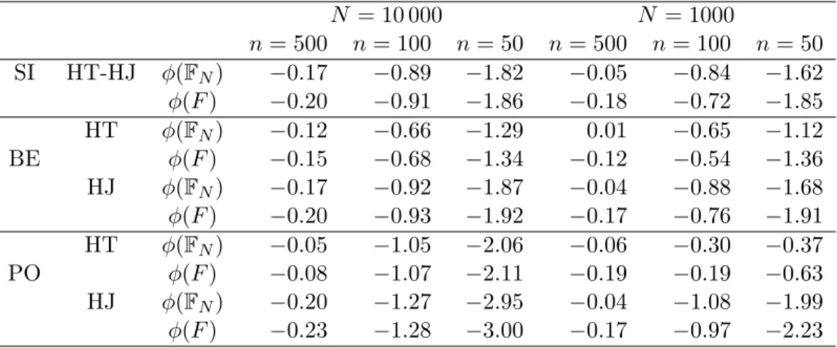
Table 1: RB (in %) of the HT and the HJ estimators for the finite population
φ(FN) and the super-populationφ(F) poverty rate parameter
N = 10 000 N = 1000 n= 500 n= 100 n= 50 n= 500 n= 100 n= 50 SI HT-HJ φ(FN) −0.17 −0.89 −1.82 −0.05 −0.84 −1.62 φ(F) −0.20 −0.91 −1.86 −0.18 −0.72 −1.85 HT φ(FN) −0.12 −0.66 −1.29 0.01 −0.65 −1.12 BE φ(F) −0.15 −0.68 −1.34 −0.12 −0.54 −1.36 HJ φ(FN) −0.17 −0.92 −1.87 −0.04 −0.88 −1.68 φ(F) −0.20 −0.93 −1.92 −0.17 −0.76 −1.91 HT φ(FN) −0.05 −1.05 −2.06 −0.06 −0.30 −0.37 PO φ(F) −0.08 −1.07 −2.11 −0.19 −0.19 −0.63 HJ φ(FN) −0.20 −1.27 −2.95 −0.04 −1.08 −1.99 φ(F) −0.23 −1.28 −3.00 −0.17 −0.97 −2.23
The Horvitz-Thompson estimator and H´ajek estimator forφ(F) orφ(FN) are denoted byφbHT and φbHJ, respectively. They are obtained by plugging in the empirical c.d.f.’sFHTN andFHJN , respectively, forF in expression (6.1). The empirical quantiles are calculated by using the functionwtd.quantile from the R packageHmiscfor the H´ajek estimator and by adapting the func-tion for the Horvitz-Thompson estimator. For the SI sampling design, the two estimators are the same. The performance of the estimators for the pa-rametersφ(F) andφ(FN) is evaluated using some Monte-Carlo relative bias (RB). This is reported in Table 1. When estimating the super-population parameterφ(F), ifφbij denotes the estimate (either φbHT orφbHJ) for the ith generated population and thejth drawn sample, the Monte Carlo relative bias ofφbin percentages has the following expression
RBF(φb) = 100 NRnR NR X i=1 nR X j=1 b φij −φ(F) φ(F) .
When estimating the finite population parameterφ(FN), the parameter de-pends on the generated population Ni, for each i= 1, . . . , NR, and will be denoted by φ(FNi). The Monte Carlo relative bias of φb is then computed by replacing F by FNi in the above expression. Concerning the relative biases reported in Table 1, the values are small and never exceed 3%. As expected, these values increase whenndecreases. When the centering is rel-ative toφ(FN), the relative bias is in general somewhat smaller than when centering withφ(F). This behavior is most prominent whenN = 1000 and
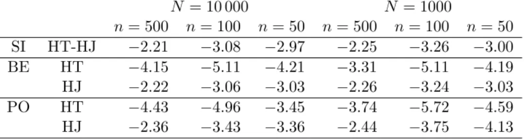
Table 2: RB (in %) for the variance estimator of the HT and the HJ esti-mators for the poverty rate parameter
N = 10 000 N = 1000 n= 500 n= 100 n= 50 n= 500 n= 100 n= 50 SI HT-HJ −2.21 −3.08 −2.97 −2.25 −3.26 −3.00 BE HT −4.15 −5.11 −4.21 −3.31 −5.11 −4.19 HJ −2.22 −3.06 −3.03 −2.26 −3.24 −3.03 PO HT −4.43 −4.96 −3.45 −3.74 −5.72 −4.59 HJ −2.36 −3.43 −3.36 −2.44 −3.75 −4.13
n= 500, which suggests that the estimates are typically closer to the pop-ulation poverty rate φ(FN) than to the model parameter φ(F). The H´ajek estimator has a larger relative bias than the Horvitz-Thompson estimator in all situations but in particular for the Poisson sampling design when the size of the population is 1000. Note that all values in Table1 are negative, which illustrates the fact that the estimators typically underestimate the population and model poverty rates.
In Table 2, the estimators of the variance of φbHT and φbHJ are obtained by plugging in the empirical c.d.f.’s FHTN and FHJN , respectively, for F in the expressions (6.3) and (6.4). To estimate f in the variance of φbHJ, we follow [5], who propose a H´ajek type kernel estimator with a Gaussian ker-nel function. For the variance of φbHT, we use a corresponding Horvitz-Thompson estimator by replacingNb by N. Based on [45], pages 45-47, we chooseb= 0.79Rn−s1/5, whereRdenotes the interquartile range. This differs from [5], who propose a similar bandwidth of the order N−1/5. However, this severely underestimates the optimal bandwidth, leading to large vari-ances of the kernel estimator. Usual bias variance trade-off computations show that the optimal bandwidth is of the ordern−s1/5.
For the SI sampling design, (6.3) and (6.4) are identical and can be calculated in an explicit way using the fact thatµπ1+λ= 1 andµπ2−λ=−1. For the BE design, µπ1+λ = 1, whereas for Poisson sampling, the value (n/N2)PN
i=11/πi is taken for µπ1+λ. For these designs, µπ2 −λ = −λ, where we take n/N as the value ofλ.
In order to compute the relative bias of the variance estimates, the asymptotic variance is taken as reference. This asymptotic variance AV(φb) of the estimator φb (either φbHT or φbHJ) is computed from (6.3) and (6.4). The expressions f(βF−1(α)) and f(F−1(α)) are explicit in the case of an exponential distribution. Furthermore, forµπ1+λ and µπ2−λwe use the
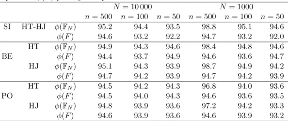
Table 3: Coverage probabilities (in %) for 95% confidence intervals of the HT and the HJ estimators for the finite population φ(FN) and the super-populationφ(F) poverty rate parameter
N = 10 000 N = 1000 n= 500 n= 100 n= 50 n= 500 n= 100 n= 50 SI HT-HJ φ(FN) 95.2 94.4 93.5 98.8 95.1 94.6 φ(F) 94.6 93.2 92.2 94.7 93.2 92.0 HT φ(FN) 94.9 94.3 94.6 98.4 94.8 94.6 BE φ(F) 94.4 93.7 94.9 94.6 93.6 94.7 HJ φ(FN) 95.1 94.3 93.9 98.7 94.9 94.2 φ(F) 94.7 94.2 93.9 94.7 94.2 93.9 HT φ(FN) 94.5 94.2 94.3 96.8 94.0 93.6 PO φ(F) 94.5 94.0 94.3 94.6 93.6 93.5 HJ φ(FN) 94.8 93.9 93.6 97.2 94.2 93.3 φ(F) 94.6 93.9 93.6 94.6 93.9 93.2
same expressions as mentioned above. The Monte Carlo relative bias of the variance estimatorAV(c φb) in percentages, is defined by
RB(AV(c φb)) = 100 NRnR NR X i=1 nR X j=1 c AV(φbij)−AV(φb) AV(φb) ,
whereAV(c φbij) denotes the variance estimate for the ith generated popula-tion and thejth drawn sample.
Table3gives the Monte-Carlo coverage probabilities for a nominal cover-age probability of 95% for the two parametersφ(FN) andφ(F), the Horvitz-Thompson and the H´ajek estimators and the different simulation schemes. In general the coverage probabilities are somewhat smaller than 95%, which is due to the underestimation of the asymptotic variance, as can be seen from Table2. The caseN = 1000 andn= 500 forφbHJ forms an exception, which is probably due to the fact that in this caseλ=n/N is far from zero, so that the limit distribution of√n(φ(FHTN )−φ(FN)) and
√
n(φ(FHJN )−φ(FN)) has a larger variance than the ones reported in Corollaries 6.1 and 6.2. When looking at Table 2, the relative biases are smaller than 5% when n is 500. The biases are larger for the Horvitz-Thompson estimator than for the H´ajek estimator. Again all relative biases are negative, which illustrates the fact that the asymptotic variance is typically underestimated.
8
Discussion
In the appendix of [36] the author remarks “To our knowledge there does not exist a general theory on conditions required for the tightness and weak convergence of Horvitz-Thompson processes.” One purpose of this paper has been to obtain these type of results in such a way that they are potentially applicable to a large class of single-stage unequal probability sampling de-signs. Conditions (C2)-(C4) play a crucial role in this, as they establish the tightness of the processes involved. The main motivation for the way they are formulated is to incorporate single-stage sampling designs which allow the sample size and/or the inclusion probabilities to depend on ω, which will be the case if they depend on the auxiliary variables Zi. These conditions trivially hold for simple sampling designs, but also for rejective sampling, which enables us to obtain weak convergence of the H´ajek and Horvitz-Thompson processes under high entropy designs. Further exten-sions to more complex designs are beyond the scope of the present investi-gation, but we believe that results similar to those described in Sections3, 4, and 5, would continue to hold under reasonable assumptions.
For instance multistage sampling designs deserve attention. The re-cent paper [18] gives some asymptotic results in the case of simple random sampling without replacement at the first stage and with arbitrary designs at further stages. [27] gives also some consistency results for a particular two-stage fixed sample size design. The clusters are drawn using sampling without replacement with a probability proportional to the size design and the secondary units are drawn using a simple random sampling without replacement within each sampled cluster. This leads to a self-weighted de-sign. Similar designs would be worth considering in order to generalize our functional limit theorems to multistage sampling.
Stratified sampling is also of importance. Asymptotics in the case of stratified simple random sampling without replacement is studied in [10], when the number of strata is bounded and in [35] when the number of strata tends to infinity. More recently, consistency results are obtained in [4] for large entropy designs when the number of strata is bounded. It would be of particular interest to generalize our functional asymptotic results to such stratified designs.
Our results rely on the assumption that the sample selection process and the super-population model characteristic are independent given the design variables. It means that the sampling is non-informative [39]. Our results do not directly generalize to informative sampling and further research is needed for such sampling designs. Also functional CLT’s for processes
correspond-ing to other estimators, such as regression and calibration estimators ([23]) deserve attention.
9
Proofs
We will use Theorem 13.5 from [11], which requires convergence of finite dimensional distributions and a tightness condition (see (13.14) in [11]. To obtain weak convergence of the finite dimensional distributions, we use con-dition (HT1) in combination with the Cr´amer-Wold device, see Lemmas9.2, 9.4, and9.6. Details of their proofs can be found in [14].
We will now establish the tightness condition, as stated in the following lemma.
Lemma 9.1. Let Y1, . . . , YN be i.i.d. random variables with c.d.f. F and
empirical c.d.f. FN and let FHTN be defined according to (2.1). Let XN = √
n(FHTN −FN) and suppose that (C1)-(C4) hold. Then there exists a
con-stant K >0 independent of N, such that for any t1,t2 and −∞< t1≤t≤
t2<∞, Ed,m h (XN(t)−XN(t1))2(XN(t2)−XN(t))2 i ≤K F(t2)−F(t1) 2 . Proof. First note that
XN(t) = √ n N N X i=1 ξi πi −1 1{Yi≤t}.
For the sake of brevity, for −∞ < t1 ≤ t ≤ t2 < ∞, and i = 1,2, . . . , N, we define p1 = F(t)−F(t1), p2 = F(t2)−F(t), Ai = 1{t1<Yi≤t}, and
Bi = 1{t<Yi≤t2}. Furthermore, let αi = (ξi −πi)Ai/πi and βi = (ξi −
πi)Bi/πi. Then, according to the fact thatp1p2 ≤(F(t2)−F(t1))2, due to the monotonicity of F, it suffices to show
1 N4Ed,m n2 N X i=1 αi !2 N X j=1 βj 2 ≤Kp1p2. (9.1) The expectation on the left hand side can be decomposed as follows
N X i=1 N X k=1 Ed,mn2α2iβ2k + N X i=1 X j6=i N X k=1 Ed,mn2αiαjβ2k + N X k=1 X l6=k N X i=1 Ed,mn2α2iβkβl + N X i=1 X j6=i N X k=1 X l6=k Ed,mn2αiαjβkβl . (9.2)
Note that by symmetry, sums two and three on the right hand side can be handled similarly, so that essentially we have to deal with three summations. We consider them one by one.
First note that, since 1{t1<Yi≤t}1{t<Yi≤t2} = 0, we will only have
non-zero expectations when{i, j} and {k, l}are disjoint. With (C1), we find
1 N4 N X i=1 N X k=1 Ed,mn2α2iβ2k = 1 N4 X X (i,k)∈D2,N Ed,mn2α2iβk2 = 1 N4 X X (i,k)∈D2,N Em n2AiBk πi2πk2Ed(ξi−πi) 2(ξ k−πk)2 ≤ 1 K4 1 X X (i,k)∈D2,N Em AiBk n2 Ed(ξi−πi) 2(ξ k−πk)2 (9.3)
Straightforward computation shows thatEd(ξi−πi)2(ξk−πk)2 equals (πik−πiπk)(1−2πi)(1−2πk) +πiπk(1−πi)(1−πk).
Hence, with (C1)-(C2) we find that
Ed(ξi−πi)2(ξk−πk)2 ≤ |Ed(ξi−πi)(ξk−πk)|+K22 n2 N2 =O n2 N2 , ω-almost surely. It follows that
1 N4 N X i=1 N X k=1 Ed,mn2α2iβ2k ≤O 1 N2 X X (i,k)∈D2,N Em[AiBk].
Since D2,N has N(N −1) elements and Em[AiBj] =p1p2 for (i, j) ∈D2,N, it follows that 1 N4 N X i=1 N X j=1 Ed,mn2α2iβj2 ≤Kp1p2. (9.4)
Similarly to (9.12), we can then write 1 N4 N X i=1 X j6=i N X k=1 Ed,mn2αiαjβ2k = 1 N4 X X X (i,j,k)∈D3,N Ed,mn2αiαjβk2 ≤ 1 N4 X X X (i,j,k)∈D3,N Ed,m n2AiAjBk πiπjπk2 (ξi−πi)(ξj−πj)(ξk−πk)2 ≤ 1 N4 X X X (i,j,k)∈D3,N Em n2AiAjBk πiπjπ2k Ed(ξi−πi)(ξj−πj)(ξk−πk) 2 ≤ 1 K4 1 X X X (i,j,k)∈D3,N Em AiAjBk n2 Ed(ξi−πi)(ξj −πj)(ξk−πk) 2 .
We find thatEd(ξi−πi)(ξj−πj)(ξk−πk)2 equals
(1−2πk)Ed(ξi−πi)(ξj−πj)(ξk−πk) +πk(1−πk)Ed(ξi−πi)(ξj−πj) With (C1)-(C3), this means |Ed(ξi −πi)(ξj −πj)(ξk−πk)2| = O(n2/N3),
ω-almost surely. It follows that
1 N4 N X i=1 X j6=i N X k=1 Ed,mn2αiαjβk2 =O 1 N3 X X X (i,j,k)∈D3,N Em[AiAjBk].
Since D3,N has N(N −1)(N −2) elements and Ed,m[AiAjBk] = p21p2, for (i, j, k)∈D3,N, we find 1 N4 N X i=1 X j6=i N X k=1 Ed,mn2αiαjβ2k ≤Kp1p2. (9.5)
The computations for the third summation in (9.2) are completely similar. Finally, consider the last summation in (9.2). As before, this summation can be bounded by 1 K14 X (i,j,k,l)∈D4,N Em AiAjBkBl n2 Ed(ξi−πi)(ξj−πj)(ξk−πk)(ξl−πl) .
SinceD4,N hasN(N−1)(N−2)(N−3) elements andEm[AiAjBkBl] =p21p22, for (i, j, k, l)∈D4,N, with (C4) we conclude that
1 N4 N X i=1 X j6=i N X k=1 X l6=k Ed,mn2αiαjβkβl ≤Kp1p2. (9.6)
Together with (9.4), (9.5) and decomposition (9.2), this proves (9.1).
Lemma 9.2. LetXN = √
n(FHTN −FN)and suppose that
(C1)-(C2),(HT1)-(HT2) hold. For anyk∈ {1,2, . . .}, andt1, . . . , tk∈R, XN(t1), . . . ,XN(tk)
converges in distribution under Pd,m to a k-variate mean zero normal
ran-dom vector with covariance matrix ΣHT
k given in (3.4).
Proof. The proof can be found in [14].
Proof of Theorem3.1 We first considerXN = √
n(FHTN −FN) for the case that theYi’s follow a uniform distribution on [0,1]. We apply Theorem 13.5 from [11]. Lemma9.2provides the limiting distribution of the finite dimen-sional projections (XN(t1), . . . ,XN(tk)), which is the same as that of the vector (GHT(t1), . . . ,GHT(tk)), where GHTis a mean zero Gaussian process with covariance function
EmGHT(s)GHT(t) = lim N→∞ 1 N2 N X i=1 N X j=1 Em nπij−πiπj πiπj 1{Yi≤s}1{Yj≤t} ,
for alls, t∈R. Tightness condition (13.14) in [11] is provided by Lemma9.1. Since GHT is continuous at 1, the theorem now follows from Theorem 13.5 in [11] for the case that theYi’s are uniformly distributed on [0,1].
To extend this to a functional CLT with i.i.d. random variablesY1, Y2, . . . with a general c.d.f. F, we can follow the argument in the proof of Theo-rem 14.3 from [11]. First define the generalized inverse ofF:
ϕ(s) = inf{t:s≤F(t)},
that satisfiess≤F(t) if and only ifϕ(s)≤t. This means that if U1, U2, . . . are i.i.d. uniformly distributed on [0,1], ϕ(Ui) has the same distribution asYi, so that 1{Yi≤t} d =1{ϕ(Ui)≤t} =1{Ui≤F(t)}. It follows that XN(t) = √ n ( 1 N N X i=1 ξi1{Yi≤t} πi − 1 N N X i=1 1{Yi≤t} ) d =ZN(F(t)), t∈R, where ZN(t) = √ n N N X i=1 ξi πi −1 1{Ui≤t}, t∈[0,1], (9.7)
Hence, the general HT empirical process XN is the image of the HT uni-form empirical processZN under the mapping ψ:D[0,1]7→D(R) given by
[ψx] (t) =x(F(t)). Note that, if xN →x inD[0,1] in the Skorohod topol-ogy and x has continuous sample paths, then the convergence is uniform. But then also ψxN converges toψx uniformly in D(R). This implies that
ψxN converges toψx in the Skorohod topology. We have established that
ZN ⇒Z weakly in D[0,1] in the Skorohod topology, where Z has continu-ous sample paths. Therefore, according to the continucontinu-ous mapping theorem, e.g., Theorem 2.7 in [11], it follows thatψ(ZN)⇒ψ(Z) weakly. This proves the theorem for Yi’s with a general c.d.f.F. 2 The proof of Proposition 3.1 is similar to that of Theorem 3.1 and can be found in [14].
To establish tightness for the process√n(FHTN −F) we use the following decomposition √ n(FHTN −F) = √ n(FHTN −FN) + √ n √ N · √ N(FN −F). (9.8)
The first process on the right hand side converges weakly to Gaussian pro-cess, according to Theorem 3.1. The process √N(FN −F) also converges weakly to a Gaussian process, due to the classical Donsker theorem. In particular both processes on the right hand side are tight inD(R) with the Skorohod metric. In general the sum of two tight processes in D(R) is not necessarily tight. However, this will be the case if both processes converge weakly to continuous processes (see LemmaB.2in [14]).
Lemma 9.3. Let V1, V2, . . . be a sequence of bounded i.i.d. random variables
on(Ω,F,Pm)with meanµV and varianceσV2, and letSN2 be defined by (3.2).
Suppose (HT1) and (HT3) hold and nSN2 → σ2HT > 0 in Pm-probability.
Then, √ n 1 N N X i=1 ξiVi πi −µV ! , (9.9)
converges in distribution underPd,m to a mean zero normal random variable
with variance σHT2 +λσV2.
Proof. The proof can be found in [14].
Lemma 9.4. Let XFN = √
n(FHTN −F) and suppose that
(C1)-(C2),(HT1)-(HT4) hold. Then for anyk∈ {1,2, . . .}, andt1, t2, . . . , tk∈R, the sequence XFN(t1), . . . ,XFN(tk)
converges in distribution under Pd,m to a k-variate
mean zero normal random vector with covariance matrixΣF
where ΣHTk is given in (3.4) and ΣF is the k×k matrix with (q, r)-entry
F(tq∧tr)−F(tq)F(tr), for q, r= 1,2, . . . , k.
Proof. The proof can be found in [14].
Proof of Theorem 3.2 The proof is completely similar to that of The-orem 3.1. We first consider the process XFN =
√
n(FHTN −F) for the case that theYi’s follow a uniform distribution withF(t) =t. DecomposeXFN as in (9.8). By Theorem 3.1, the first process on the right hand side of (9.8) converges weakly to a process in C[0,1]. Due to the classical Donsker the-orem and (HT3), the second process on the right hand side of (9.8) also converges weakly to a process inC[0,1]. Tightness ofXFN then follows from Lemma B.2 in [14]. Convergence of the finite dimensional distributions is provided by Lemma9.4. The theorem now follows from Theorem 13.5 in [11] for the case that the Yi’s are uniformly distributed on [0,1]. Next, this is extended toYi’s with a general c.d.f. F in the same way as in the proof of
Theorem3.1. 2
To establish convergence in distribution of the finite dimensional dis-tributions of √n(FHTN −F) under the conditions of Proposition 3.2, as in the proof of Lemma 9.4, we will use the Cram´er-Wold device. To ensure thatnS2
N still has a strictly positive limit without imposing (HT4), we will need the following lemma. Its proof can be found in [14].
Lemma 9.5. Let F be the c.d.f. of the i.i.d. Y1, . . . , YN. For any k-tuple (t1, . . . , tk) ∈ Rk, suppose that the values F(t1), . . . , F(tk) are all distinct
and such that 0 < F(ti) <1. Let a, b∈R, such that a≥b. If a >0, then the k×kmatrix Mwith(i, j)-th element Mij =aF(ti∧tj)−bF(ti)F(tj) is
positive definite.
Lemma 9.6. Let XFN = √
n(FHTN −F) and suppose that n and πi, πij,
for i, j = 1,2, . . . , N, are deterministic. Suppose that (C1)-(C2), (HT1) and (HT3) hold, as well as conditions (i)-(ii) of Proposition 3.2. Then, for any k ∈ {1,2, . . .}, and t1, . . . , tk ∈ R, XFN(t1), . . . ,XFN(tk)
converges in distribution under Pd,m to a k-variate mean zero normal random vector
with covariance matrix ΣFHT, with (q, r)-entry (µπ1+λ)F(tq∧tr) + (µπ2−
λ)F(tq)F(tr), for q, r,= 1,2, . . . , k.
Proof. The proof can be found in [14].
The proof of Proposition 3.2 is similar to that of Theorem 3.2 and can be found in [14].
Proof of Theorem 4.1 For part (i), note that with S2N defined in (3.2) withVi= 1, from (HT1) together with condition (4.6), it follows that
√ nSN × 1 SN 1 N N X i=1 ξi πi −1 ! →N(0, σ2π), ω−a.s.,
in distribution underPd. This implies
√ n Nb N −1 ! =√n 1 N N X i=1 ξi πi −1 ! →N(0, σπ2), (9.10)
in distribution underPd,m. In particular, sincen→ ∞, this proves part (i). The proof of part(ii) is along the same lines as the proof of Theorems3.1 and 3.2. First consider the case, where theYi’s are uniform, withF(t) = t
on [0,1]. Then, withFHTN defined in (2.1) and XFN = √
n(FHTN −F), we can write GπN(t) = XFN(t)−(XFN(t)−GπN(t)). According to Theorem 3.2, the process XFN converges weakly to a continuous process. As a consequence of (9.10), the process XFN(t)−GπN(t) =t √ n 1 N N X i=1 ξi πi −1 ! ,
also converges weakly to a continuous process. Hence, similar to the argu-ment in the proof of Theorem3.2, we conclude that the processGπN is tight. Next, we establish weak convergence of the finite dimensional projections.
Details can be found in [14]. 2
Proof of Theorem4.2 We use (4.2). From the proof of Theorem4.1, we know that GπN is tight. Together with Theorem4.1(i), it then follows that the limit behavior of√n(FHJN −FN) is the same as that of the process YN defined in (4.3). This process can be written as
YN(t) = √ n N N X i=1 ξi πi −1 1{Yi≤t}−F(t) √ n N N X i=1 ξi πi −1 .
As in the proofs of Theorems3.1,3.2, and 4.1, we first consider the case of uniformYi’s. The first process on the right hand side is
√
n(FHTN −FN), which converges weakly to a continuous process, according to Theorem3.1, whereas the second process also converges to a continuous process due to (9.10). As in the proof of Theorem3.2, one can then argue thatYN, being the difference
of these processes, is tight. Next, we prove weak convergence of the finite dimensional projections. Details can be found in [14]. 2 The proofs of Propositions 4.1 and 4.2 are similar to those of Theo-rems4.2and 4.1, respectively, and can be found in [14].
Proof of Corollary 5.1 Similar to the approach followed in [3], we first prove the results for a rejective sampling R and then extend them to high entropy designs.
First note thatEd(ξi−πi)(ξj−πj) =πij−πiπj. According to Theorem 1 in [13], which is an extension of Theorem 5.2 in [32], together with (C1) and (A2), for sampling designR,
πij−πiπj =πiπj − 1 dN (1−πi)(1−πj) +O(d−N2) =O(n2/(N2dN)), (9.11)
ω-almost surely. Therefore, together with (A3), condition (C2) follows,
ω-almost surely. For condition (C3), according to Lemma 2 in [13], the third order correlation Ed(ξi −πi)(ξj −πj)(ξk −πk) splits into terms of the form (πij −πiπj)πk and the term πijk−πiπjπk. Similar to (9.11), to-gether with Theorem 1 in [13], the latter term can be shown to be of the order O(n3/(N3dN)), whereas other terms are of the same order according to (C1)-(C2) and (A2). Again, together with (A3), condition (C3) follows,
ω-almost surely. According to Proposition 1 in [13],
|Ed(ξi−πi)(ξj−πj)(ξk−πk)(ξl−πl)|=O(d−N2), a.s.−Pm. Hence, together with (A4), condition (C4) follows, ω-almost surely. Theo-rems 3.1 and 3.2 are now immediate, when either (HT2) holds or (HT2)-(HT4), respectively, which establishes parts (i) and (ii) for the rejective sampling design R. For parts (iii) and (iv), it can be seen that under de-signR, n N2 X X i6=j πij −πiπj πiπj =− n N2 X X i6=j (1−πi)(1−πj) dN +O n/d2N =− n N2d N (N −n)2+O(1/dN) +O n/d2N →α,
with (A2)-(A3) and (A5). Hence, Theorems 4.2 and 4.3 are now immedi-ate with µπ2 = −α, when either (HT3) and (HJ2) hold or (HT3), (HJ2),
and (HJ4), respectively, which establishes parts (iii) and (iv) for rejective sampling designR.
To extend these results to high entropy designs, we use the same ap-proach as in [7]. They use the bounded Lipschitz metric for random elements
X and Y on a metric spaceD:
dBL(X, Y) = sup f∈BL1
|Ef(Y)−Ef(X)|,
where BL1 is the class of Lipshitz functions with Lipshitz norm bounded by one. See [48], page 73, who define the metricdBL on the space of separable Borel measures. Weak convergence is metrizable by this metric, i.e.,
Xα X ⇔ sup
f∈BL1
|E∗f(Xα)−Ef(X)| →0.
Now, consider part (i) and let P be a high entropy design. Let R be some rejective sampling design such thatD(PkR)→0. Given the inclusion prob-abilitiesπ1(P), . . . , πN(P), there exists a rejective sampling design Re such that πi(Re) = πi(P). Note that D(PkRe) ≤ D(PkR) → 0, according to Lemma 3 in [3].
Consider the Horvitz-Thompson process for the designP
GπP(P)(t) = √ n 1 N N X i=1 ξi(P)1{Yi≤t} πi(P) − 1 N N X i=1 1{Yi≤t} ! ,
and compare this with the same process for design ˜R,
Gπ(P) e R (t) = √ n 1 N N X i=1 ξi(Re)1{Yi≤t} πi(P) − 1 N N X i=1 1{Yi≤t} ! .
Then, because Ed[ξi(P)] = Ps∈SNP(s)δi(s), where δi(s) = 1 when i ∈ s and zero otherwise, it follows that forEdf(GπP(P)), the argument inside f is independent of the designP. Hence, for any f ∈BL1, one finds
Edf GπP(P) −EdfGπ(P) e R ≤ X s∈P(UN) |P(s)−Re(s)| ≤ q 2D(PkRe),
using Lemma 2 in [3]. As|Ed,mf(Y)−Ed,mf(X)| ≤Em|Edf(Y)−Edf(X)|, it follows that dBL1(G
π(P) P ,G
π(P) e
established for rejective sampling design Re, we obtain that G π(P) e R → G weakly. Hence,dBL1(G π(P) e R ,G)→0 and therefore dBL1(G π(P) P ,G)≤dBL1(G π(P) P ,G π(P) e R ) +dBL1(G π(P) e R ,G)→0
which means that GπP(P) → G weakly. This establishes part(i) for high entropy designP. Parts (ii)-(iv) are obtained in the same way. 2
Proof of Corollary 5.3 We first re-prove Lemma 9.1 under conditions (C2∗)-(C4∗). Because n is deterministic, it can be taken out of the expec-tation Ed,m. When also π1, . . . , πN are deterministic, this means that the expectationEd over theξi’s can be separated from the expectationEm over theAi’s andBj’s in (9.2). It follows that
1 N4 N X i=1 N X k=1 Ed,mn2α2iβk2 = n 2 N4 X X (i,k)∈D2,N Ed(ξi−πi)2(ξk−πk)2 πi2πk2 p1p2. (9.12)
Straightforward computation shows thatEd(ξi−πi)2(ξk−πk)2 equals (πik−πiπk)(1−2πi)(1−2πk) +πiπk(1−πi)(1−πk).
The contribution of the last term is
n2 N4 X X (i,k)∈D2,N πiπk(1−πi)(1−πk) π2 iπk2 ≤ n N2 N X i=1 1 πi −1 !2 =O(1),
according to condition (i) of Proposition 3.1. With (C1) and (C2∗), the contribution of the first term is
n2 N4 X X (i,k)∈D2,N (πik−πiπk)(1−2πi)(1−2πk) π2iπ2k ≤O N2 n2 n2 N4 ·N X i6=k πik−πiπk πiπk =O 1 n . (9.13) This establishes (9.4).
For the second (and third) summation on the right hand side of (9.2), we have 1 N4 N X i=1 X j6=i N X k=1 Ed,mn2αiαjβk2 ≤ n 2 N4 X X X (i,j,k)∈D3,N Ed (ξi−πi)(ξj−πj)(ξk−πk)2 πiπjπk2 p1p2
We still have thatEd(ξi−πi)(ξj−πj)(ξk−πk)2 equals
(1−2πk)Ed(ξi−πi)(ξj−πj)(ξk−πk) +πk(1−πk)Ed(ξi−πi)(ξj−πj). The contribution of the last term is
n2 N4 X X X (i,j,k)∈D3,N 1 πk −1 πij −πiπj πiπj ≤ n N2 X X (i,j)∈D2,N πij −πiπj πiπj · n N2 N X k=1 1 πk −1 =O(1),
according to conditions (i)-(ii) of Proposition 3.1. From Lemma 2 in [13], we have thatEdξi−πi)(ξj−πj)(ξk−πk) splits into
1. −(πij −πiπj)πk−(πik−πiπk)πj −(πjk−πjπk)πi. 2. πijk−πiπjπk.
According to (C1) and (C2∗), the contribution of the terms in the first case is of the orderO(1) similarly to (9.13), whereas (C1) and (C3∗) yield that the contribution of the second case is also of the order O(1). This establishes (9.5). Finally, 1 N4 N X i=1 X j6=i N X k=1 X l6=k Ed,mn2αiαjβkβl = n 2 N4 X (i,j,k,l)∈D4,N Ed[(ξi−πi)(ξj−πj)(ξk−πk)(ξl−πl)] πiπjπkπl p21p22.
Because 0 ≤ p1, p2 ≤ 1, together with (C4∗), we obtain (9.6). Together with (9.4), (9.5) and decomposition (9.2), this proves Lemma9.1.