Clemson University
Clemson University
TigerPrints
TigerPrints
Publications
School of Computing
10-2019
Multilevel Combinatorial Optimization Across Quantum
Multilevel Combinatorial Optimization Across Quantum
Architectures
Architectures
Hayato Ushijima-Mwesigwa
Fujitsu Laboratories of America
Ruslan Shaydulin
Clemson University
Christian F.A. Negre
Los Alamos National Laboratory
Susan M. Mniszewski
Los Alamos National Laboratory
Yuri Alexeev
Argonne National Laboratory
See next page for additional authors
Follow this and additional works at:
https://tigerprints.clemson.edu/computing_pubs
Part of the
Computer Sciences Commons
Recommended Citation
Recommended Citation
Ushijima-Mwesigwa, Hayato; Shaydulin, Ruslan; Negre, Christian F.A.; Mniszewski, Susan M.; Alexeev, Yuri;
and Safro, Ilya, "Multilevel Combinatorial Optimization Across Quantum Architectures" (2019).
Publications. 41.
https://tigerprints.clemson.edu/computing_pubs/41
This Article is brought to you for free and open access by the School of Computing at TigerPrints. It has been accepted for inclusion in Publications by an authorized administrator of TigerPrints. For more information, please contact [email protected].
Authors
Authors
Hayato Ushijima-Mwesigwa, Ruslan Shaydulin, Christian F.A. Negre, Susan M. Mniszewski, Yuri Alexeev,
and Ilya Safro
HAYATO USHIJIMA-MWESIGWA
∗†‡,
Fujitsu Laboratories of America, Inc.RUSLAN SHAYDULIN
∗†,
School of Computing, Clemson UniversityCHRISTIAN F. A. NEGRE,
Theoretical Division, Los Alamos National LaboratorySUSAN M. MNISZEWSKI,
Computer, Computational, & Statistical Sciences Division, Los Alamos National LaboratoryYURI ALEXEEV,
Computational Science and Leadership Computing Divisions, Argonne National LaboratoryILYA SAFRO
†,
School of Computing, Clemson UniversityEmerging quantum processors provide an opportunity to explore new approaches for solving traditional problems in the Post Moore’s law supercomputing era. However, the limited number of qubits makes it infeasible to tackle massive real-world datasets directly in the near future, leading to new challenges in utilizing these quantum processors for practical purposes. Hybrid quantum-classical algorithms that leverage both quantum and classical types of devices are considered as one of the main strategies to apply quantum computing to large-scale problems. In this paper, we advocate the use of multilevel frameworks for combinatorial optimization as a promising general paradigm for designing hybrid quantum-classical algorithms. In order to demonstrate this approach, we apply this method to two well-known combinatorial optimization problems, namely, the Graph Partitioning Problem, and the Community Detection Problem. We develop hybrid multilevel solvers with quantum local search on D-Wave’s quantum annealer and IBM’s gate-model based quantum processor. We carry out experiments on graphs that are orders of magnitudes larger than the current quantum hardware size and observe results comparable to state-of-the-art solvers.
Reproducibility: Our code and data are available at [1]
CCS Concepts: •Mathematics of computing→Graph algorithms;Combinatorial optimization; •Hardware→Quantum computation.
Additional Key Words and Phrases: NISQ, Quantum Annealing, Graph Partitioning, Modularity, Community Detection
1 INTRODUCTION
Across different domains, computational optimization problems that model large-scale complex systems often introduce
a major obstacle to solvers even if tackled with high-performance computing systems. There are several reasons for this,
including but not limited to a large number of variables and even larger number of interactions, and dimensionality
required to describe each variable or interaction, and time slices. The combinatorial and mixed integer optimization
problems introduce additional layers of complexity with integer variables often making the problem NP-hard (e.g., in
cases of non-linearity and non-convexity). A common practical approach to solve these problems is to use iterative
∗
Both authors contributed equally to this work.
†
Corresponding authors.
‡
Work on this paper was in part performed while the author was affiliated with Clemson University.
Authors’ addresses: Hayato Ushijima-Mwesigwa, [email protected], Fujitsu Laboratories of America, Inc. Sunnyvale, CA, 94085; Ruslan Shaydulin, [email protected], School of Computing, Clemson University, Clemson, SC, 29634; Christian F. A. Negre, Theoretical Division, Los Alamos National Laboratory, Los Alamos, NM, 87545, [email protected]; Susan M. Mniszewski, Computer, Computational, & Statistical Sciences Division, Los Alamos National Laboratory, Los Alamos, NM, 87545, [email protected]; Yuri Alexeev, Computational Science and Leadership Computing Divisions, Argonne National Laboratory, Argonne, IL, 60439; Ilya Safro, [email protected], School of Computing, Clemson University, Clemson, SC, 29634.
methods. The iterative methods, while being composed with completely different algorithmic principles, share a common
property: several fast improvement iterations followed by a long tail of slow improvement iterations [27, 63]. Typically,
in such iterative algorithms, solving a large-scale system with respect to the first-order interaction laws per iteration
advances the solution towards a local attraction basin at each iteration, which often appears to be false with respect
to the global optimal solution. In other words, local methods tend to converge to a false local optimum, which often
corresponds to the solution of lower quality than the true global optimum [23]. Moreover, in some cases, another
problem may exist within each iteration – the algorithms used to solve them are not necessarily exact. To accelerate the
solvers at each iteration various heuristics, parallelization-friendly methods, and ad-hoc tricks are employed, which
often reduce the quality of the solution.
In this paper, we take steps towards building more robust solvers for mid- to large-scale combinatorial optimization
problems by fusing two areas whose simultaneous application is only beginning to be explored, namely, quantum
computing and multiscale methods. Recent advances in quantum computing provide a new approach for algorithm
development for many combinatorial optimization problems. However, Noisy Intermediate Scale Quantum (NISQ)
devices are widely expected to be limited to a few hundred, and for certain sparse architectures up to a few thousands
qubits. The current state of quantum computing theory and engineering suggests moderately optimistic expectations.
In particular, it is believed that in the near future, we will witness relatively robust architectures with much less noise.
This would allow algorithms like the Quantum Approximate Optimization Algorithm (QAOA) and Quantum Annealing
(QA) to be run on hardware with limited error correction. Given the realistic level of precision and, in the case of
QAOA, ansatz depth, these algorithms are prime candidates for demonstrating Quantum Advantage, that is solving a
computationally hard problem (such as NP-hard) faster than classical state-of-the-art algorithms. Such algorithms are
our first building block.
The multiscale optimization method is our second building block. These methods have been developed to cope
with large-scale problems by introducing an approach to avoid entering false local attraction basins (local optima), a
complementary method to stochastic and multi-start strategies that help to escape it if trapped. Because of historical
reasons, on graph problems, they have been termedmultilevel(rather than multiscale), which we will use here. The multilevel (or multiscale) methods have a long history of breakthrough results in many different optimization problems
[10, 13, 16, 18, 20, 25, 31, 32, 43, 44, 46–49, 52, 53] and have been implemented on a variety of hardware architectures.
The success of multilevel methods for optimization problems supports our optimism about proposed ideas.
There is no unique prescription on how to design multilevel algorithms, but the main idea behind them is to “think
globally while acting locally” on a hierarchy of coarse representations of the original large-scale optimization problem. A
multilevel algorithm therefore begins by constructing such a hierarchy of progressively smaller (coarser) representations
of the original problem. The goal of the next coarser level in this hierarchy is to approximate the current level problem
with a coarser one that has fewer degrees of freedom and thus can be solved more effectively. When the coarse problem
is solved, its solution is projected back to the finer level and further refined, a stage that is called uncoarsening. As a
result of such a strategy, the multilevel framework is often able to significantly improve the running time and solution
quality of optimization methods. The quality of multilevel algorithms in large part depends on that of the optimization
solvers applied at all stages of the multilevel framework. In many cases, these locally acting optimization solvers are
either heuristics that get stuck in a local optimum or exact solvers applied on a small number of variables (i.e., on
subproblems). In both cases, the quality of a global solution can significantly suffer depending on the quality of the
solution from the local solver. The optimization algorithms running on the NISQ devices that may replace such local
solvers are expected to be a critical missing component to achieve a game changing breakthrough in multilevel methods
for combinatorial optimization.
In this paper, we introduce Multilevel Quantum Local Search (ML-QLS), which uses an iterative refinement scheme
on NISQ devices within a multilevel framework. ML-QLS extends the Quantum Local Search (QLS) [55, 56] approach to
solve larger problems. This work builds on early results using a multilevel framework and the D-Wave quantum Annealer
for the Graph Partitioning Problem [61]. We demonstrate the general approach of solving combinatorial optimization
problems with NISQ devices in a multilevel framework on two well-known problems as our use cases. In particular, we
solve the Graph Partitioning Problem and the Community Detection Problem on graphs up to approximately 29,000 nodes using subproblem sizes of 20 and 64 that map onto NISQ devices such as IBM Q Poughkeepsie (20 qubits) and
D-Wave 2000Q (∼2048 qubits). Such graphs are orders of magnitude larger than those solved by state-of-the-art hybrid quantum-classical methods. To implement this approach, we develop a novel efficient subproblem formulation method.
In contrast, some of the authors of this paper have previously developed quantum and quantum-classical algorithms
for the Graph Partitioning Problem and the Community Detection Problem for multiple parts (> 2) [33, 60]. These did
not use a multilevel approach, instead anall at onceor concurrent approach was employed.
The rest of paper is organized as follows. In Section 2, we discuss the relevant background on quantum optimization,
multilevel methods, and define the problems. In Sections 3 and 4, we discuss the hybrid quantum-classical multilevel
algorithm and computational results, respectively. A discussion of the outlook and important open problems that
represent major future research directions are presented in Section 5.
2 BACKGROUND
The methods proposed and implemented in this work aim to solve large graph problems by integrating NISQ optimization
algorithms into a multilevel scheme. In this section, we provide a brief introduction into all three components: target
graph problems (Sec. 2.1), quantum optimization (Sec. 2.2) and multilevel methods (Sec. 2.3)
Many optimization problems discussed in this work are posed in Ising form. The Ising model is a common
math-ematical abstraction to represent the energy ofndiscrete spin variablesσi ∈ {−1,1}, 1≤i≤n, and interactionsJij betweenσiandσj. For each spin variableσi, a local fieldhi is specified. The energy of a configurationσis given by the Hamiltonian function: H(σ)=Õ i,j Jijσiσj+Õ i hiσi, σi ∈ {−1,1}. (1)
An equivalent mathematical formulation is the Quadratic Unconstrained Binary Optimization (QUBO) problem. The
objective of a QUBO problem is to minimize (or maximize) the following function:
H(x)=Õ i<j Qijxixj+ Õ i Qiixi, x ∈ {0,1}. 2.1 Problem Definitions
LetG=(V,E)be an undirected graph with vertex setV and edge setE. We denote bynandmthe numbers of nodes and edges, respectively. For each nodei, definevi ∈Ras the volume of nodeiandAij∈Ras the positive weight of edge(i,j). For a fixed integerk, theGraph Partitioning Problemis to find a partitionV1, . . . ,Vkof the vertex setVintok parts with equal total node volume such that the total weight ofcut edgesis minimized. Acut edgeis defined as an edge whose end points are in different partitions. A requirement of equal total sizes ofVifor alliis sometimes referred as Manuscript submitted to ACM
perfectly balancedgraph partitioning, otherwise an imbalancing parameter is usually introduced to allow imbalanced partitions [12]. However, in this work we deal with perfect balancing constraints and limit the number of parts tok=2. In this case we can write the GP problem as the following quadratic program
max sTAs s.t. n Õ i=1 visi =0 si ∈ {−1,1},i=1, . . . ,n, (2)
which, as shown in [60], can be reformulated into the following Ising model,
max sT(βA−αvvT)s s.t. si ∈ {−1,1},i=1, . . . ,n,
(3)
for some constantsα,β>0, wherevis a column vector of volumes such that(v)i=vi.
Maximization of modularity is a famous problem in network science where the goal is to find communities in
a network through node clustering (also known as modularity clustering) [34]. For the graphG, the problem of Modularity Maximization is to find a partitioning of the vertex set into one or more parts (communities) that maximizes
the modularity metric. The modularity matrix is a symmetric matrix given by
Bij =Aij−kikj 2|E|,
(4)
whereki is the weighted degree of nodei, namely,ki = ÍjAij. Whereas the modularity is typically defined on unweighted graphs, within the multilevel framework, due to the coarsening of nodes, we primarily work with weighted
graphs. It can equivalently be written in matrix-vector notation as
B=A− 1 2|E|kk
T (5)
wherekis a vector of weighted degrees of the nodes in the graph. For up to 2 communities, theModularity Maximization
Problem, also referred to as theCommunity Detection Problem, can be written in Ising form as follows:
max 1 4|E|s T A− 1 2|E|kk T s s.t. si ∈ {−1,1}, i=1, . . . ,n (6)
where the objective value of equation 6, for a given assignment of resulting communities, is referred to as themodularity. For more than 2 communities, the Ising formulation of the Community Detection Problem is given in [33].
Note that the above formulation of Modularity Maximization can be viewed as the Graph Partitioning Problem in
the Ising model given in equation (3) where the volume of a node is defined as the weighted degree and the penalty
constantsβ=1,α= 1 2|E|
. We exploit this deep duality between the two problems in our implementation.
2.2 Optimization on NISQ devices
In recent years we have seen a number of advances in quantum optimization algorithms that can be run on NISQ
devices. Two most prominent ones are the Quantum Approximate Optimization Algorithm (QAOA) and Quantum
Annealing (QA), which are inspired by the adiabatic theorem. There are many formulations of the adiabatic theorem
(see [6] for a comprehensive review), but all of them stem from the adiabatic approximation formulated by Kato in
1950 [26]. Adiabatic approximation states, roughly, that a system prepared in an eigenstate (e.g. a ground state) of
some time-dependent HamiltonianH(t)will remain in the corresponding eigenstate1provided thatH(t)is varied “slowly enough”. The requirement on the evolution time scales asO(1/∆2)in the worst case [15], where∆is the minimum eigengap between ground and first excited state ofH(t). Adiabatic Quantum Computation (AQC) is quantum Merlin-Arthur (QMA)-complete [6] and is equivalent to gate-based universal quantum computation.
Quantum Annealing is a special case of AQC limited to stochastic Hamiltonians The transverse field Hamiltonian
HM =
Õ
i
σix (7)
is used as the initial Hamiltonian. The final Hamiltonian is a classical Ising model Hamiltonian with the ground state
encoding the solution of the original problem:
HC =Õ ij
Jijsisj+Õ i
hisi, si ∈ {−1,+1}.
The evolution of the system starts in the ground state ofHMand it is described by a time-dependent Hamiltonian
H(t)= t
THC+(1− t
T)HM,t ∈ (0,T). (8)
QAOA extends the logic of AQC to gate-model quantum computers and can be interpreted as a discrete approximation
of the continuous QA schedule, performed by applying two alternating operators:
W(βk)=e−i βkHMandV(γk)=e−iγkHC.
W(βk)corresponds to evolving the system with HamiltonianHM for a period of timeβk andV(γk)corresponds to evolvingHCfor timeγk. Similarly to QA, the evolution begins in the ground state ofHM, namely|+⟩⊗n. Alternating operators are applied to produce the state:
|ψ(β,γ)⟩=e−i βpHMe−iγpHC. . .e−i β1HMe−iγ1HC |+⟩⊗n=U(β,γ) |+⟩⊗n. (9) An alternative implementation was proposed, inspired by the success of the Variational Quantum Eigensolver
(VQE) [41]. A variational implementation of QAOA combines an ansatzU(β,γ)(that can be different from the alternating operator one described above) and a classical optimizer. A commonly used ansatz is a hardware-efficient ansatz [24],
consisting of alternating layers of entangling and rotation gates. The algorithm starts by preparing a trial state by
applying the parameterized gates to some initial state:|ψ(β,γ)⟩=U(β,γ) |+⟩⊗n. In the next step, the state|ψ(β,γ)⟩ is measured and the classical optimization algorithm uses the result of the measurement to choose the next set of
parametersβ,γ. The goal of the classical optimization is to find the parametersβ,γcorresponding to the optimal QAOA “schedule”, i.e. the schedule that produces the ground state of the problem HamiltonianHC:
β∗,γ∗=arg min β,γ
⟨ψ(β,γ)|HC|ψ(β,γ)⟩. (10) Both QA and QAOA have been successfully implemented in hardware by a number of companies, universities and
national laboratories [5, 14, 35, 37, 38, 42].
1
A note on terminology: a HamiltonianHis a Hermitian operator. The spectrum ofHcorresponds to the potential outcomes if one was to measure the energy of the system described byH.|ψ⟩is an eigenstate of a system described by HamiltonianHwith energyλ∈RifH|ψ⟩=λ|ψ⟩. In other words, |ψ⟩is an eigenvector ofHwith real eigenvalueλ.
2.3 Multilevel Combinatorial Optimization
The goal of the multilevel approach for optimization problems on graphs is to create a hierarchy of coarsened graphsG0,
G1, ... ,Gkin such a way that the next coarser graphGi+1“approximates” some properties ofGi(that are directly relevant to the optimization problem of interest) but with fewer degrees of freedom. After constructing such a hierarchy, the
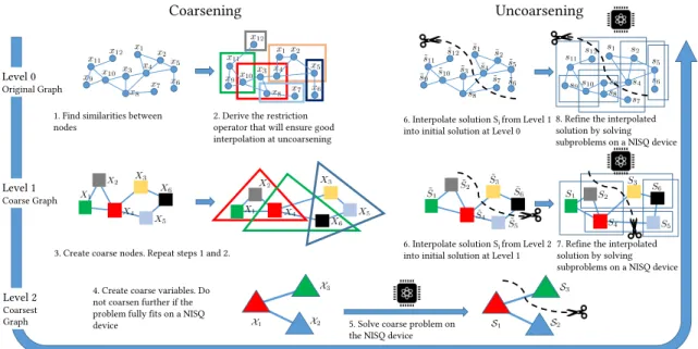
coarsening is followed by solving the problem onGkas best as we can (preferably exactly) do and finally uncoarsening the solution back toG0through gradual refinement at all levels of the hierarchy, with a refined solution at leveli+1 serving as the initial solution at leveli. The entire coarsening-uncoarsening process is called a V-cycle. There are other variations of hierarchy levels’ coarsening-uncoarsening order, e.g., W- and Full cycles [11]. Fig. 1 presents an outline of
a V-cycle.
Typically, when solving problems on graphs in which nodes represent the optimization variables (such as those in
the partitioning and Community Detection), having fewer degrees of freedom implies a decreased number of nodes in
each next coarser graph|V0|>|V1|>|V2|> ... >|Vk|. 2
With a smaller number of variables at each level, one can use
more sophisticated algorithms at each level. However, it is still not sufficient to solve the original problem as a whole
until the coarsening reaches the coarsest level. As a result, at each level, the actual solution is produced by a refinement.
Refinement is typically implemented with a decomposition method that uses a previous iteration or a coarser level
solution as an initial guess. The multilevel algorithms rely heavily [64] on the quality of refinement solvers for small
and local subproblems at all levels of coarseness. Thus, the most straightforward way to use NISQ devices in multilevel
frameworks is to iteratively apply them as local solvers to refine a solution inherited from the coarse level. Because the
refinement is executed at all levels of coarseness, it is clear thateven a small improvement of a solution at the coarse level
2
Note that this does not necessarily imply|E0|> |E1|>|E2|> ... >|Ek|
Coarsening Uncoarsening Level 0 Original Graph Level 1 Coarse Graph Level 2 Coarsest Graph
1. Find similarities between
nodes 2. Derive the restriction operator that will ensure good interpolation at uncoarsening
3. Create coarse nodes. Repeat steps 1 and 2. 4. Create coarse variables. Do not coarsen further if the problem fully fits on a NISQ
device 5. Solve coarse problem on the NISQ device
6. Interpolate solution Si from Level 2
into initial solution at Level 1 7. Refine the interpolated solution by solving subproblems on a NISQ device 6. Interpolate solution Si from Level 1
into initial solution at Level 0 8. Refine the interpolated solution by solving subproblems on a NISQ device
Fig. 1. V-cycle for a graph problem. First, the problem is iteratively coarsened (left). Second, the coarse problem is solved using a NISQ optimization solver (bottom). Finally, the problem is iteratively uncoarsened and the solution is refined using a NISQ solver (right).
may cause a major improvement at the finest scale. Typically, this is the most time-consuming stage of the multilevel process which is expected to be fundamentally better if improved by NISQ devices. Most refinement solvers in multilevel
frameworks rely on fast but low-quality heuristics, rather than on the ability to compute an optimal solution. Moreover,
in many existing solvers, the number of variables in such local subproblems is comparable with or smaller than the the
size of the problems that can be directly embedded on the NISQ devices (see examples in [20, 28, 31]), making them a
perfect target for NISQ optimization algorithms. In most multilevel/multiscale/multigrid-based optimization solvers, a
refinement consists of covering the domain (or all variables) withsmallsubsets of variables (i.e., small subproblems) such that solving a small local problem on a subset improves the global solution for the current level.
Multilevel Graph Partitioning and Community Detection algorithms are examples of the most successful applications
of multilevel algorithms for large graphs, achieving excellent time/quality performance [12]. In this paper, we use the
simplest version of coarsening (in order to focus on the hybrid quantum-classical refinement) in which the edges of the
fine level graph are collapsed and create coarse level vertices by merging the fine level ones. There are several classes of
refinement for both problems but in all of them, at each step a small subset of nodes (or even a singleton) is reassigned
with partition (or cluster) that either better optimizes the objective or improves constraints. Some variants of stochastic
extensions also exist.
3 METHODS
An iterative improvement scheme is a common approach for solving large scale problems with NISQ devices.
Tradi-tionally, this is done by formulating the entire problem in the Ising model or as a QUBO and then solving it using
hybrid quantum-classical algorithms (see, for example, "qbsolv" from D-Wave systems [8]). These methods decompose
the large QUBO into smaller sub-QUBOs or decrease the number of degrees of freedom to fit the subproblem on the
hardware (for example, using a multilevel scheme), and iteratively improve the global solution by solving the small
subproblems (sub-QUBOs). One of the main limitations of this approach is the size and density of the original QUBO.
For example, in the graph partitioning formulation given by equation 3, the termvvT leads to the formulation of a completely densen×nQUBO matrix regardless of whether or not the original graph was sparse. Storing and processing this dense matrix can easily make this method prohibitively computationally expensive even for moderately sized
problems. In our implementation of Quantum Local Search (QLS) [56] we circumvent this limitation by developing a
novel subproblem formulation of the Graph Partitioning Problem and Modularity Maximization as a QUBO that does
not require formulating the entire QUBO.
Another concern is the effectiveness of selection criteria of candidate variables (or nodes) to be included in each
subproblem. A common metric used in selecting whether or not a variable is to be included in the subproblem is whether
or not changing the variable value would reduce (increase) the objective value for a minimization (maximization)
problem. Thus, since computing the change in objective value for a small change in the solution is performed multiple
times, it is important to ensure that this computation is efficient. We derive a novel efficient way to compute the change
in the objective value of the entire QUBO also without formulating the entire QUBO and thus provide an efficient
refinement scheme using current NISQ devices.
We begin by introducing an efficient QUBO subproblem formulation for the Graph Partitioning Problem, and the
Community Detection Problem. Then we present an efficient way to compute the gain and change in the objective of
the entire QUBO. Finally, we put it all together and outline our algorithm.
3.1 QUBO formulation for subproblems
LetMbe ann×nsymmetric matrix that represents the QUBO for a large scale problem such that it is prohibitively expensive to either generate or storeM. However, for QLS we need to generate constant-size sub-QUBOs ofMwhich in turn represent subproblems of the original problem. In order to generate a sub-QUBO, letkbe the size of the desired sub-QUBO. In other words, the sub-QUBO will havekvariables andn−kfixed variablesthat remain invariant for this specific sub-QUBO. We refer to thekvariables asfree variables. Without loss of generality, let the the firstkvariables of sbe the free variables, then we writesas
s= " sv sf # ,
wheresv represents thekfree variable terms andsf represents then−kfixed terms. In the next step,Mcan be represented using block form
M= Mvv Mvf MT vf Mf f (11)
such thatMvvis ak×kmatrix. Next, we can writesTMsas
sTMs=sTvMvvsv+sTv(2Mvfsf)+sT
fMf fsf (12)
Sincesf are fixed values, we havesT
fMf fsf as a constant thus
minsTMs=min sTvMvvsv+sTv(2Mvfsf) (13) From equation (11), we have
vvT = vvvTv vvvTf vfvTv vfvTf (14)
Therefore, from equation (13), we have
min sTvvTs=minsTvvvvTvsv+2sTvvvvT
fsf (15)
The formulation in (15) is particularly important because it shows that the matrixvvT does not need to be explicitly created at each iteration during refinement. This is a crucial observation becausevvT is a completely dense matrix.
As described in Sec. 2.1, the Community Detection Problem is given by
max 1 4|E|s T A− 1 2|E|kk T s (16)
or minsT 1 2|E|kk T −A s (17)
and the Graph Partitioning Problem is given by
minsT
αvvT −βAs. (18)
In the above formulation, modularity clustering can be viewed as the Graph Partitioning Problem in a QUBO model,
where the volume of a node is defined as the weighted degree and the penalty constant is 1
|E|Therefore, in both cases we can perform a refinement while defining fixed values as
minsT 1 2|E|kk T −A s=minsTv 1 2|E|kvk T v sv+sTv 1 |E|kvk T f sf −sTAs (19) and minsT αvvT −βAs=min sTv αvvvTv sv+sTv2αvvvT f sf −βsTAs (20) with
min−βsTAs=min−βsTvAvvsv−sTv(2βAvfsf) (21) The formulation in (19) and (20) are particularly important during the refinement step because this implies that the
complete dense (and therefore prohibitively large) QUBO or Ising model does not need to be created at each iteration.
These formulations also demonstrate a close relationship between the Graph Partitioning Problem and the Community
Detection Problem.
3.2 Efficient Evaluation of the Objective
In order to select the free variables for the subproblem, we need to be able to efficiently compute the change of the
objective function by moving one node from one part to another. In other words, for each vertexv, we need to efficiently compute thegainwhich is the decrease (or increase) in the edge-cut together with penalty ifvis moved to the other part.
For a symmetric matrixM, the change in the valueQ=sTMsby flipping a single variablesi corresponding to the nodeiis given by ∆Q(i)=2( Õ j∈C1 Mij−Õ j∈C2 Mij) (22)
whereC1andC2correspond to all variables withsi=−1 andsi =1 respectively. Next, we define
deд(v,C):= Õ j∈C Av j; Deд(C):= Õ i∈C ki; Vol(C):= Õ i∈C vi then 2( Õ j∈C1 Aij−Õ j∈C2 Aij)=2deд(vi,C1) −2deд(vi,C2) and finally 2( Õ j∈C1 (vvT)ij−Õ j∈C2 (vvT)ij)=2 vi Õ j∈C1,i,j vj−vi Õ j∈C2 vj =2vi Vol(C1\i) −Vol(C2)
where we assume thati∈C1. This expression can be computed inO(1)time.
In the same way 2( Õ j∈C1 (kkT)ij− Õ j∈C2 (kkT)ij)=2 ki Õ j∈C1,i,j kj−ki Õ j∈C2 kj =2ki Deд(C1\i) −Deд(C2)
can also be computed inO(1)time givenDeд(C1)andDeд(C2), whereDeд(Ci)represents the sum of weighted degrees of nodes in communityi.
Therefore, the change in modularity is given by
∆Q(i)= ki |E| Deд(C1\i) −Deд(C2) −2 deд(vi,C1) −deд(vi,C2) (23)
and change in edge-cut together with penalty value is given by
∆Q(i)=2αvi Vol(C1\i) −Vol(C2) ) −2β deд(vi,C1) −deд(vi,C2) (24)
For each nodei, both expressions (23) and (24) can be computed inO(ki)time, whereki is the unweighted degree of
i.
At no point during the algorithm should the complete QUBO matrix be formulated. This also applies to the process
of evaluating a given solution. In other words, evaluating the modularity for the Community Detection Problem or
edge-cut together with penalty term for the Graph Partitioning Problem should be done inO(1)time and space. The term is sTvvTs= Vol(C1) −Vol(C2) 2 where as sTAs=2(|E| −2cut). Therefore,
sT(αvvT −βA)s=αVol(C1) −Vol(C2) 2 −2β(|E| −2cut) (25) and sT 1 2|E|kk T −A s= 1 2|E| Deд(C1) −Deд(C2) 2 −2(|E| −2cut) (26) where equations (25) and (26) give the formulations for computing the modularity and edge-cut with corresponding
penalty value respectively without creating the QUBO matrix.
3.3 Algorithm Overview
Now we can combine the building blocks described in the previous two subsections. LetG=(V,E)be the problem graph. ML-QLS begins by coarsening the problem graph. During the coarsening stage, for some integerk, a hierarchy of coarsened graphsG=G0,G1, . . . ,Gkis constructed. In this work, we used the coarsening tools implemented in KaHIP Graph Partitioning package [51]. We used the coarsening implementation that is performed using maximum weight
matching with “expansion∗2” metric as described in [22]. The maximum edge matching is found using the Global Path
Algorithm [22]. In the next step, a QUBO is formulated for the smallest graphGkand solved on the quantum device. If |Vk|is greater than the hardware size3, QLS [56] with a random initialization is used to solve forGk. Then, the solution is iteratively projected onto finer levels and refined using QLS. The algorithm overview is presented in Alg. 1.
3
more specifically, greater than the maximum number of variables in a problem that can be embedded on the device Manuscript submitted to ACM
Algorithm 1Multilevel Quantum Local Search functionML-QLS(G, problem_type)
ifproblem_type is modularitythen
G= UpdateWeights(G) G0,G1, . . . ,Gk= KaHIPCoarsen(G) if|Vk| ≤HardwareSizethen //solve directly QUBO = FormulateQUBO(Gk) solution = SolveSubproblem(QUBO) else //use QLS initial_solution = RandomSolution(Gk) solution = RefineSolution(Gk, initial_solution) forGi inGk−1,Gk−2, . . . ,G0do
projected_solution = ProjectSolution(solution,Gi,Gi+1) solution = RefineSolution(Gi, projected_solution) returnsolution
functionRefineSolution(Gi, projected_solution) solution = projected_solution
whilenot convergeddo
∆Q= ComputeGains(Gi, solution)
X= HighestGainNodes(∆Q) QUBO = FormulateQUBO(X)
//using IBM UQC or D-Wave QA
candidate = SolveSubproblem(QUBO) ifcandidate>solutionthen
solution = candidate returnsolution
For the Graph Partitioning Problem, the initial weight of each node is one by definition, therefore coarsening of the
nodes keeps the total node volume constant at each coarsening level. For the Community Detection Problem, the initial
weight of each node is set to the degree of the node. This ensures that the size of the graph (total number of weighted
edges) is also kept constant at each level. Note that Graph Partitioning is defined with respect to total node volume
(|V|), while modularity is defined with respect to the size (|E|, the total number of weighted edges) of the graph.
3.4 Addressing the Limited Precision of the Hardware
One of the subproblem solvers we used in this work is Quantum Annealing, which we ran on the LANL D-Wave 2000Q
machine. The D-Wave 2000Q is an analog quantum annealer with limited precision. In this work, we used a simple
coarsening that constructs coarser graphs by aggregating nodes at a finer level to become a single node at the coarser
level (i.e. many nodes on the finer level are merged into one node at the coarser level, with the volume of the new node
set to be the sum of the volumes of the nodes on the coarser level). This causes the precision required to describe the
node volumes and edge weights for coarser graphs to increase dramatically, especially for the large scale problems. Thus,
a QUBO describing the coarsest graph could require significantly more precision to represent compared to the finest
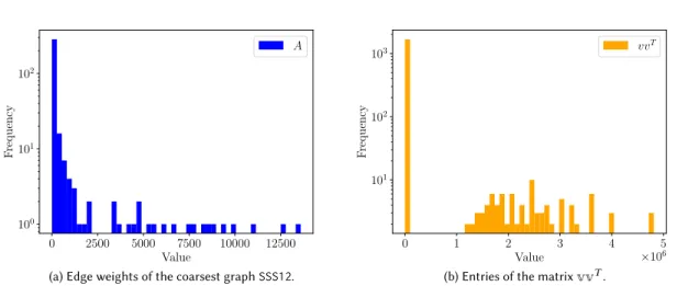
graph. For example, in Graph Partitioning where the QUBO problem to be minimized isA−αvvT, the range of values in the matrixAincrease at a different rate than the range of values in the matrixvvT during the coarsening process, Manuscript submitted to ACM
0 2500 5000 7500 10000 12500 Value 100 101 102 F requency A
(a) Edge weights of the coarsest graphSSS12.
0 1 2 3 4 5 Value ×106 101 102 103 F requency vvT
(b) Entries of the matrixvvT.
Fig. 2. In Figure 2a, the maximum value is approximately13×103.In Figure 2b, the maximum value is approximately5×106and
minimum value1. A naive scaling of QUBO matrixA−vvT can result in values that are too large to be handled by the quantum
annealer due to its limited precision. Such values ofAare ignored, leading to random balanced partitions.
increasing the precision required to describe the overall QUBO formed at each level (see an example on Fig. 2a). Thus, if
the QUBOA−αvvT is directly scaled to accommodate the limited precision of the device, the quality of the results can suffer. In our experiments, we observe that directly scaling the QUBO returned feasible, but low quality solutions. In
order to overcome this challenge, for the problems solved on the D-Wave device, we first scaled the matricesAand
αvvT separately, and then formed the QUBO to be optimized. This approach then resulted in achieving results with high quality solutions on the D-Wave device.
4 EXPERIMENTS AND RESULTS
Implementation.The general framework for ML-QLS is implemented in Python 3.7 with NetworkX [19] for network
operations. We have used the coarsening algorithms available in the KaHIP Graph Partitioning package [51] which are
implemented in C++. The code for the general ML-QLS framework is available on GitHub [1].
Systems. The refinement algorithms presented in this work require access to NISQ devices capable of solving problems
formulated in the Ising model. To this end, we have used the D-Wave 2000Q quantum annealer located at Los Alamos
National Laboratory, as well as IBM’s Poughkeepsie 20 qubit quantum computer available on the Oak Ridge National
Laboratory IBM Q hub network together with the high-performance simulator, IBM Qiskit Aer Simulator [7]. However,
our framework is modular and can easily be extended to utilize other novel quantum computing architectures as they
become available.
The D-Wave 2000Q is the state-of-the-art quantum annealer at this time. It has up to 2048 qubits which are laid out in a
special graph structure known as a Chimera graph. The Chimera graph is sparse, thus the device has sparse connectivity.
Fully connected graphs as dense problems need to be embedded onto the device, which leads to the maximum size
of 64 variables. We have used the embedding algorithm described in [9] to calculate a complete embedding of the 64
variable problem. We found this embedding only once and reused it during our experiments. We utilized D-Wave’s
Solver API (SAPI) which is implemented in Python 2.7, to interact with the system. The D-Wave system is intrinsically
a stochastic system, where solutions are sampled from a distribution corresponding to the lowest energy state. For each
subproblem, the best solution out of 10,000 samples is returned. The annealing time for each call to the D-Wave system
was set to 20 microseconds.
In order to solve problems formulated in the Ising model on IBM’s Poughkeepsie quantum computer and simulator,
we implemented QAOA using the SBPLX [45] optimizer to find the optimal variational parameters. We allowed 2000
iterations for SBPLX to find optimal parameters for QAOA run on the simulator and 250 iterations for QAOA on the
device. Due to the limitations of NISQ devices available in IBM Q hub network [54], we used the RYRZ variational
form [3] (also known as a hardware-efficient ansatz) as the ansatz for our QAOA implementation. For the experiments
run on IBM quantum device Poughkeepsie, we perform the variational parameter optimization on the simulator locally
and run QAOA on the device via the IBM Q Experience cloud API. This is done due to the job queue limitations provided
via the IBM Q Experience. However, we expect to be able to run QAOA variational parameter optimization fully on
a device as more devices are becoming available on the cloud. We have used GNU Parallel [59] for the large-scale
numerical experiments performed on the quantum simulator.
Considering the fact that solutions from the NISQ devices and simulator do not provide optimality guarantees,
we have also solved various subproblems formulated in the Ising model using the solver Gurobi [36] together with
modeling package Pyomo [21]. The results using Gurobi as a solver for each subporblem are denoted as "Optimal" in
our plots to highlight the point that each subproblem was solved and proven to be optimal.
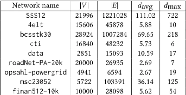
Instances. A summary of the graphs used in the experimentes together with their properties is presented in
Ta-ble 1. For the Graph Partitioning ProTa-blem, we evaluate ML-QLS on five graphs, four of which are drawn from The
Graph Partitioning Archive [58] (4elt,bcsstk30,ctianddata) and one from the set of hard to partition graphs (vsp_msc10848_300sep_100in_1Kout, denoted in figures asSSS12) [49]. For the Modularity Maximization Problem, we evaluate ML-QLS on six graphs. The graphsroadNet-PA-20kandopsahl-powergridare real-world networks from the KONECT dataset [29]. Graphsmsc23052andfinan512-10kare taken from the graph archive presented in [50]. The graphsfinan512-10kandroadNet-PA-20kare reduced to 10,000 and 20,000 nodes respectively by performing a breadth-first search from the median degree node. Note that due to the high diameter of these networks and their
structure (portfolio optimization problem and road network), this preserves their structural properties.GirvanNewmanis a synthetic graph generated using the model introduced by Girvan and Newman (GN) [17]. The graphlancichinetti1 is a synthetic graph generated using a generalization of the GN model that allows for heterogeneity in the distributions
of node degree and community size, introduced by Lancichinetti et al. [30]. Table 2 shows the parameters used to
generate the synthetic graphs.
Experimental Setup.Our experiments are performed in order to compare the solutions from ML-QLS with those
of high-quality classical solvers, and the best known results, if available. For the Graph Partitioning Problem, the
results are compared to those produced by KaHIP [51] which is a state-of-the-art multilevel Graph Partitioning
solver. The best known results are taken at The Graph Partitioning Archive [58] where applicable. In order to make
our approach more comparable to KaHIP, we follow the user guide [4], and use thekaffpaEversion of the solver with the option--mh_enable_kabapEfor high quality refinement for perfectly balanced parts. We use the option
--preconfiguration=fastto ensure results are compared with a single V-cycle. Our results (cut values) are normalized with either the best known value when applicable or by the smallest cut value found by any of the solvers used.
Network name |V| |E| davg dmax SSS12 21996 1221028 111.02 722 4elt 15606 45878 5.88 10 bcsstk30 28924 1007284 69.65 218 cti 16840 48232 5.73 6 data 2851 15093 10.59 17 roadNet-PA-20k 20000 26935 2.69 7 opsahl-powergrid 4941 6594 2.67 19 msc23052 5722 103391 36.14 125 finan512-10k 10000 28098 5.62 54
Table 1. Properties of the networks used to evaluate ML-QLS.davg is average degree,dmax is maximum degree
Network name |V| |E| davg dmax γ β µ
GirvanNewman 10,000 75,000 15.0 15 1 1 0.1
lancichinetti1 10,000 76,133 15.22 50 2 1 0.1
Table 2. Properties of synthetic networks used in the Modularity evaluation.davg is average degree,dmax is maximum degree,γis the exponent for the degree distribution,βis the exponent for the community size distribution andµis the mixing parameter. For a detailed discussion of the parameters the reader is referred to Ref. [30]
Network name Best modularity
finan512-10k 0.499 GirvanNewman 0.459 lancichinetti1 0.452 msc23052 0.499 opsahl-powergrid 0.497 roadNet-PA-20k 0.499
Table 3. Highest modularity value found by all methods for a given problem. The highest possible modularity value for at most 2 communities is 0.5.
For the Modularity Maximization Problem, we compare our solutions using ML-QLS with two classical clustering
methods, Asynchronous Fluid Communities [39] (implemented in NetworkX [19]) and Spectral Clustering [57, 62]
(implemented in Scikit-learn [40]). Note that even though these methods solve the same problem (namely, Community
Detection or clustering), they do not explicitly maximize modularity. Therefore, it is unfair to directly compare the
modularity of the solution produced by them to ML-QLS, which is explicitly maximizing modularity. However, they
provide a useful baseline. Moreover, since the maximum possible modularity for at most 2 communities is 0.5, the best
solutions found by all methods are no more than 1%–10% away from the optimal (see Table 3)
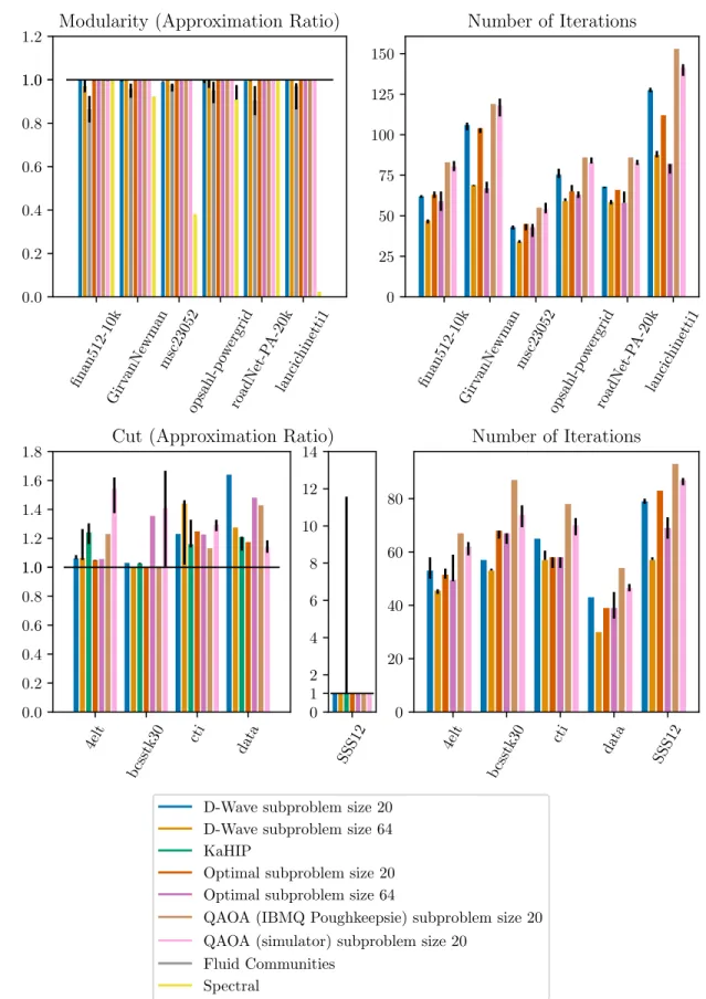
The experimental results are presented in Figure 4. We have made all raw result data available on Github [2]. For
each problem and method (except for QAOA on IBM Q Poughkeepsie quantum computer, labeled “QAOA (IBMQ
Pough-keepsie)” in Figure 4), we perform ten runs of a single V-cycle with different seeds. For “QAOA (IBMQ PoughPough-keepsie)”,
we perform just one run per each problem due to the limited access to quantum hardware.
Observations.We observe that ML-QLS is capable of achieving results close to the best ones found by other solvers
for all problems. For Graph Partitioning, Figure 4 shows significant variability in the quality of the solution across
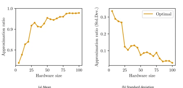
0 25 50 75 100 Hardware size 0.8 0.9 1.0 Appro ximation ratio (a) Mean 0 25 50 75 100 Hardware size 0.1 0.2 0.3 Appro ximation ratio (Std.Dev.) Optimal (b) Standard deviation
Fig. 3. Modularity (Approximation ratio) as the function of the size of the subproblem (hardware size). The performance is projected using Gurobi as the subproblem solver and allowing it to solve each subproblem to optimality. The top plot presents the mean approximation ratio averaged over the entire benchmark. The bottom plot presents the standard deviation. As the hardware size increases, the quality of the solution found by ML-QLS improves.
different solvers and problem instances. This effect is also observed for the state-of-the-art Graph Partitioning solver
KaHIP, when run for a single V-cycle. This is partially due to the fact that we normalize the objectives to make them
directly comparable. For example, for the graph4eltthe best known cut value presented in The Graph Partitioning Archive [58] is 139. Therefore, anabsolutedifference of 28 edges in cut obtained by a solver translates into a 20%relative difference presented in Figure 4. However, the sameabsolutedifference of 28 edges would translate into≈0.44% for the graphbcsstk30(best known cut 6394). The graphSSS12is specifically designed to be hard for traditional Graph Partitioning frameworks [49]. This explains the high variation in the performance of KaHIP on it.
It is worth noting that QAOA on the IBM quantum computers (see “QAOA (IBM Q Poughkeepsie)” in Figure 4) takes
more iterations to converge to a solution compared to D-Wave. This is partially due to the fact that we perform the
QAOA variational parameter optimization on the simulator and only run once with the optimized parameters on the
device. As a result, the learned variational parameters do not include the noise profile of the device, limiting the quality
of subproblem solutions. As devices become more easily available, we expect to be able to run full variational parameter
optimization on the quantum hardware.
To project the performance improvements for future hardware, we simulate the performance of ML-QLS as a function
of hardware (subproblem) size shown in Figure 3. As the subproblem size increases, the average quality of the solution
found by ML-QLS improves and variation in results decreases. This shows that performance of ML-QLS can be improved
as larger size quantum devices and better quantum optimization routines are developed.
16 Ushijima-Mwesigwa and Shaydulin, et al. finan512-10k Girv anNewmanmsc23052 opsahl-p ow ergrid roadNet-P A-20k lancic hinetti1 0.0 0.2 0.4 0.6 0.8 1.0 1.2 1.0 finan512-10k Girv anNewmanmsc23052 opsahl-p ow ergrid roadNet-P A-20k lancic hinetti1 0 25 50 75 100 125 150 4elt bcsstk30 cti data 0.0 0.2 0.4 0.6 0.8 1.0 1.2 1.4 1.6 1.8 1.0 SSS12 0 2 4 6 8 10 12 14 1 4elt bcsstk30 cti data SSS12 0 20 40 60 80
Number of Iterations
Cut (Approximation Ratio)
D-Wave subproblem size 20 D-Wave subproblem size 64 KaHIP
Optimal subproblem size 20 Optimal subproblem size 64
QAOA (IBMQ Poughkeepsie) subproblem size 20 QAOA (simulator) subproblem size 20
Fluid Communities Spectral
Fig. 4. Quality of the solution and the number of iterations for all problems and solvers. The height of the bars is the median over 10 seeds. Error bars (black) are 25th and 75th percentiles. For the objective function (Cut or Modularity) all results are normalized by the best solution found by any solver (for Graph Partitioning this includes the best known cuts from The Graph Partitioning Archive [58]). Number of iterations is the number of calls to the subproblem solver (ML-QLS only).
5 OPEN PROBLEMS AND DISCUSSION
Revising (un)coarsening operators in anticipation of the new class of high-quality refinement solvers is the first major
open problem. The majority of multilevel algorithms for combinatorial optimization problems are inspired by the idea of
"thinking globally while acting locally". However, there is a crucial difference between these algorithms for combinatorial
problems and such methods as multigrid for continuous problems or multiscale PDE-based optimization. In multigrid
(e.g., for systems of linear equations), a relaxation at the uncoarsening stage is convergent [10], and in most cases assumes
an optimal solution (up to some tolerance) for a subset of relaxed variables given other variables are invariant (i.e., a fixed
solution for those variables that are not in the optimized subset). Examples include easily parallelizable Jacobi relaxation,
as well as hard to parallelize Gauss-Seidel relaxation in which most variables are typically optimized sequentially,
and many more. Both coarsening and uncoarsening operators (also known as the restriction, and prolongation in
multigrid) assume this convergence which in the end provides guarantees for the entire multilevel framework. However,
for thecombinatorialmultilevel solvers, the integer variables make this assumption practically impossible, even for subproblems containing tens of variables optimized simultaneously. With the development of noiseless NISQ devices,
we can assume that in our hands will be extremely fast heuristics to produce nearly (if hypothetically not completely)
optimal solutions for combinatorial optimization problems of up to several hundreds variables. In order to use the
multilevel paradigm correctly, there will be a critical need to revise (un)coarsening operators that take this feature into
account because (to the best of our knowledge) all existing versions of coarsening operators do not consider optimality
of the refinement. Moreover, most existing multilevel frameworks exhibit more emphasis on computational speedup
rather than on the quality of the solution to better approximate the fine problem.
The second problem is not unique to multilevel methods but to most decomposition based approaches. Even if
quantum devices become fully developed and become more accessible for the broad scientific community, they will
still remain more expensive than regular CP U based devices. The decomposition approaches split the problem into
many small local subproblems, while multilevel methods may need even more of them because solving subproblems
is required at all levels of coarseness. Thus, there is a critical need in developing an extremely fast routing classifier
for a subproblem that will decide whether solving a particular subproblem on the NISQ device will be beneficial in
comparison to the CP U.
6 CONCLUSION
Current Noisy Intermediate-Scale Quantum (NISQ) devices are limited in the number of qubits and can therefore only
be used to directly solve combinatorial optimization problems that exhibit a limited number of variables. In order to
overcome this limitation, in this work we have proposed the multilevel computational framework for solving large-scale
combinatorial problems on NISQ devices. We demonstrate this approach on two well-known combinatorial optimization
problems, the Graph Partitioning Problem, and the Community Detection Problem, and perform experiments on the 20
qubit IBM gate-model quantum computer, and the 2048 qubit D-Wave 2000Q quantum annealer. In order to implement
an efficient iterative refinement scheme using the NISQ devices, we have developed novel techniques for efficiently
formulating and evaluating sub-QUBOs without explicitly constructing the entire QUBO of the large-scale problem,
which in many cases can be a dense matrix that makes it computationally expensive to store and process. In our
experiments, for the Graph Partitioning Problem, five graphs were chosen such that the smallest graph had 2851 nodes
while the largest had 28924 nodes, while for the Community Detection Problem, the smallest graph had 4941 nodes and
largest had 10,000 nodes. For both problems, for comparison purposes, we run one V-cycle of the multilevel framework
with the different NISQ devices multiple times and compared the results to the state-of-art methods. Our experimental
results give comparable results to the state-of-the-art methods and for some cases we were able to get the best-known
results. This work therefore provides an important stepping stone to demonstrating practical Quantum Advantage.
As the capabilities of NISQ devices increase, we are hopeful that similar methods can provide a path to adoption of
quantum computers for a variety of business and scientific applications.
ACKNOWLEDGMENTS
This work was supported in part by NSF award #1522751. High-performance computing resources at Clemson University
were supported by NSF award MRI #1725573. This research used resources of the Oak Ridge Leadership Computing
Facility, which is a DOE Office of Science User Facility supported under Contract DE-AC05-00OR22725. This research
also used the resources of the Argonne Leadership Computing Facility, which is DOE Office of Science User Facility
supported under Contract DE-AC02-06CH11357. Yuri Alexeev and Ruslan Shaydulin were supported by the DOE
Office of Science. The authors would also like to acknowledge the NNSA’s Advanced Simulation and Computing (ASC)
program at Los Alamos National Laboratory (LANL) for use of their Ising D-Wave 2000Q quantum computing resource.
LANL is operated by Triad National Security, LLC, for the National Nuclear Security Administration of U.S. Department
of Energy (Contract No. 89233218NCA000001). Susan Mniszewski and Christian Negre were supported by the ASC
program at LANL. Assigned: Los Alamos Unclassified Report 19-30113.
REFERENCES
[1] [n. d.]. https://github.com/rsln- s/ml_qls
[2] [n. d.]. https://github.com/rsln- s/ml_qls/tree/bc376276ba684460aeccaa371b4fc38003139e34/multilevel/data/results_csv
[3] [n. d.]. IBM QISKit Aqua: Variatinal forms. https://github.com/Qiskit/qiskit- aqua/blob/master/qiskit/aqua/components/variational_forms/ryrz.py. [Online; accessed July 16, 2019].
[4] [n. d.]. KaHIP v2.10 – Karlsruhe High Quality Partitioning User Guide. http://algo2.iti.kit.edu/schulz/software_releases/kahipv2.10.pdf .[Online; accessed July 31, 2019].
[5] [n. d.]. Quantum Enhanced Optimization (QEO). https://www.iarpa.gov/index.php/research- programs/qeo.[Online; accessed September 25, 2018]. [6] Tameem Albash and Daniel A Lidar. 2018. Adiabatic quantum computation.Reviews of Modern Physics90, 1 (2018), 015002.
[7] Gadi Aleksandrowicz, Thomas Alexander, Panagiotis Barkoutsos, Luciano Bello, Yael Ben-Haim, et al. 2019. Qiskit: An Open-source Framework for Quantum Computing. https://doi.org/10.5281/zenodo.2562110
[8] Michael Booth, Steven P Reinhardt, and Aidan Roy. 2017. Partitioning optimization problems for hybrid classical.quantum execution. Technical
Report(2017), 01–09.
[9] Tomas Boothby, Andrew D King, and Aidan Roy. 2016. Fast clique minor generation in Chimera qubit connectivity graphs.Quantum Information
Processing15, 1 (2016), 495–508.
[10] A. Brandt. 2002. Multiscale Scientific Computation: Review 2001. InMultiscale and Multiresolution Methods. LNCSE, Vol. 20. Springer, 3–95. http://dx.doi.org/10.1007/978- 3- 642- 56205- 1_1
[11] A. Brandt and D. Ron. 2003. Chapter 1 : Multigrid solvers and multilevel optimization strategies. InMultilevel Optimization and VLSICAD, J. Cong and J. R. Shinnerl (Eds.). Kluwer.
[12] Aydın Buluç, Henning Meyerhenke, Ilya Safro, Peter Sanders, and Christian Schulz. 2016. Recent advances in graph partitioning. InAlgorithm
Engineering: Selected Results and Surveys. LNCS 9220, Springer-Verlag. Springer, 117–158. [13] J. Cong and J. R. Shinnerl (Eds.). 2003.Multilevel Optimization and VLSICAD. Kluwer.
[14] D-Wave Systems Inc. 2018. Introduction to the D-Wave Quantum Hardware. (2018). www.dwavesys.com/tutorials/background- reading-series/introduction- d- wave- quantum- hardware
[15] Alexander Elgart and George A. Hagedorn. 2012.A note on the switching adiabatic theorem.J. Math. Phys.53, 10 (Oct. 2012), 102202. https: //doi.org/10.1063/1.4748968
[16] E Gelman and J Mandel. 1990. On multilevel iterative methods for optimization problems.Mathematical Programming48, 1-3 (1990), 1–17. [17] M. Girvan and M. E. J. Newman. 2002. Community structure in social and biological networks.Proceedings of the National Academy of Sciences99,
12 (June 2002), 7821–7826. https://doi.org/10.1073/pnas.122653799
[18] Serge Gratton, Annick Sartenaer, and Philippe L Toint. 2008. Recursive trust-region methods for multiscale nonlinear optimization.SIAM Journal on
Optimization19, 1 (2008), 414–444. Manuscript submitted to ACM
[19] Aric A. Hagberg, Daniel A. Schult, and Pieter J. Swart. 2008. Exploring Network Structure, Dynamics, and Function using NetworkX. InProceedings
of the 7th Python in Science Conference (SciPy 2008), Gaël Varoquaux, Travis Vaught, and Jarrod Millman (Eds.). Pasadena, CA USA, 11–15. [20] William W Hager, James T Hungerford, and Ilya Safro. 2018. A multilevel bilinear programming algorithm for the vertex separator problem.
Computational Optimization and Applications69, 1 (2018), 189–223.
[21] William E Hart, Carl D Laird, Jean-Paul Watson, David L Woodruff, Gabriel A Hackebeil, et al. 2017.Pyomo-optimization modeling in python. Vol. 67. Springer.
[22] Manuel Holtgrewe, Peter Sanders, and Christian Schulz. 2010. Engineering a scalable high quality graph partitioner. In2010 IEEE International
Symposium on Parallel & Distributed Processing (IPDPS). IEEE. https://doi.org/10.1109/ipdps.2010.5470485
[23] Reiner Horst, Panos M Pardalos, and Nguyen Van Thoai. 2000.Introduction to global optimization. Springer Science & Business Media. [24] Abhinav Kandala, Antonio Mezzacapo, Kristan Temme, Maika Takita, Markus Brink, et al. 2017. Hardware-efficient variational quantum eigensolver
for small molecules and quantum magnets.Nature549, 7671 (2017), 242.
[25] G. Karypis and V. Kumar. 1999. A Fast and High Quality Multilevel Scheme for Partitioning Irregular Graphs.SIAM Journal on Scientific Computing 20, 1 (1999).
[26] Tosio Kato. 1950. On the Adiabatic Theorem of Quantum Mechanics.Journal of the Physical Society of Japan5, 6 (Nov. 1950), 435–439. https: //doi.org/10.1143/jpsj.5.435
[27] Carl T Kelley. 1999.Iterative methods for optimization. SIAM.
[28] Y. Koren and D. Harel. 2002. Multi-Scale Algorithm for the Linear Arrangement Problem.Proceedings of 28th Inter. Workshop on Graph-Theoretic
Concepts(2002). citeseer.nj.nec.com/koren02multiscale.html
[29] Jérôme Kunegis. 2013. Konect: the koblenz network collection. InProceedings of the 22nd International Conference on World Wide Web. ACM, 1343–1350.
[30] Andrea Lancichinetti, Santo Fortunato, and Filippo Radicchi. 2008. Benchmark graphs for testing community detection algorithms.Physical Review
E78, 4 (Oct. 2008). https://doi.org/10.1103/physreve.78.046110
[31] Sven Leyffer and Ilya Safro. 2013. Fast response to infection spread and cyber attacks on large-scale networks.Journal of Complex Networks1, 2 (2013), 183–199.
[32] Athanasios Migdalas, Panos M Pardalos, and Peter Värbrand. 2013.Multilevel optimization: algorithms and applications. Vol. 20. Springer Science & Business Media.
[33] Christian F A Negre, Hayato M Ushijima-Mwesigwa, and Susan M Mniszewski. 2019. Detecting multiple communities using quantum annealing on the D-Wave system.arXiv preprint arXiv:1901.09756(2019).
[34] M. E. J. Newman. 2006.Modularity and community structure in networks.Proceedings of National Academy of Sciences103 (2006), 8577. doi: 10.1073/pnas.0601602103
[35] Sergey Novikov, Robert Hinkey, Steven Disseler, James I Basham, Tameem Albash, et al. 2018. Exploring More-Coherent Quantum Annealing.arXiv
preprint arXiv:1809.04485(2018).
[36] Gurobi Optimization. 2014. Inc.,“Gurobi optimizer reference manual,” 2015. http://www.gurobi.com. (2014).
[37] JS Otterbach, R Manenti, N Alidoust, A Bestwick, M Block, et al. 2017. Unsupervised Machine Learning on a Hybrid Quantum Computer.arXiv
preprint arXiv:1712.05771(2017).
[38] G Pagano, A Bapat, P Becker, KS Collins, A De, et al. 2019. Quantum Approximate Optimization with a Trapped-Ion Quantum Simulator.arXiv
preprint arXiv:1906.02700(2019).
[39] Ferran Parés, Dario Garcia Gasulla, Armand Vilalta, Jonatan Moreno, Eduard Ayguadé, et al. 2017. Fluid communities: a competitive, scalable and diverse community detection algorithm. InInternational Conference on Complex Networks and their Applications. Springer, 229–240.
[40] F. Pedregosa, G. Varoquaux, A. Gramfort, V. Michel, B. Thirion, et al. 2011. Scikit-learn: Machine Learning in Python.Journal of Machine Learning
Research12 (2011), 2825–2830.
[41] Alberto Peruzzo, Jarrod McClean, Peter Shadbolt, Man-Hong Yung, Xiao-Qi Zhou, et al. 2014. A variational eigenvalue solver on a photonic quantum processor.Nature communications5 (2014), 4213.
[42] Hannes Pichler, Sheng-Tao Wang, Leo Zhou, Soonwon Choi, and Mikhail D Lukin. 2018. Quantum Optimization for Maximum Independent Set Using Rydberg Atom Arrays.arXiv preprint arXiv:1808.10816(2018).
[43] Dorit Ron, Ilya Safro, and Achi Brandt. 2010. A Fast Multigrid Algorithm for Energy Minimization under Planar Density Constraints.SIAM Multiscale
Modeling & Simulation8, 5 (2010), 1599–1620.
[44] Dorit Ron, Ilya Safro, and Achi Brandt. 2011. Relaxation-based coarsening and multiscale graph organization.Multiscale Modeling & Simulation9, 1 (2011), 407–423.
[45] Thomas Harvey Rowan. 1990.Functional stability analysis of numerical algorithms.Ph.D. Dissertation. University of Texas at Austin. [46] Ehsan Sadrfaridpour, Talayeh Razzaghi, and Ilya Safro. 2019. Engineering fast multilevel support vector machines.Machine Learning(2019), 1–39. [47] Ehsan Sadrfaridpour, Jeereddy Sandeep, Ken Kennedy, Andre Luckow, Talayeh Razzaghi, et al. 2017. Algebraic multigrid support vector machines.
InESANN 2017 proceedings, European Symposium on Artificial Neural Networks, Computational Intelligence and Machine Learning. ESANN, Bruges, Belgium. https://www.elen.ucl.ac.be/Proceedings/esann/esannpdf/es2017- 37.pdf
[48] Ilya Safro, Dorit Ron, and Achi Brandt. 2008. Multilevel algorithms for linear ordering problems.ACM Journal of Experimental Algorithmics13 (2008).
[49] Ilya Safro, Peter Sanders, and Christian Schulz. 2015. Advanced coarsening schemes for graph partitioning.ACM Journal of Experimental Algorithmics
(JEA)19 (2015), 2–2.
[50] Ilya Safro and Boris Temkin. 2011. Multiscale approach for the network compression-friendly ordering.J. Discrete Algorithms9, 2 (2011), 190–202. [51] Peter Sanders and Christian Schulz. 2013. Think Locally, Act Globally: Highly Balanced Graph Partitioning. InProceedings of the 12th International
Symposium on Experimental Algorithms (SEA’13) (LNCS), Vol. 7933. Springer, 164–175.
[52] Ruslan Shaydulin, Jie Chen, and Ilya Safro. 2019. Relaxation-Based Coarsening for Multilevel Hypergraph Partitioning.SIAM Multiscale Modeling
and Simulation17 (2019), 482–506. Issue 1.
[53] Ruslan Shaydulin and Ilya Safro. 2018. Aggregative Coarsening for Multilevel Hypergraph Partitioning. In17th International Symposium on
Experimental Algorithms (SEA 2018) (Leibniz International Proceedings in Informatics (LIPIcs)), Gianlorenzo D’Angelo (Ed.), Vol. 103. Schloss Dagstuhl–Leibniz-Zentrum fuer Informatik, Dagstuhl, Germany, 2:1–2:15. https://doi.org/10.4230/LIPIcs.SEA.2018.2
[54] Ruslan Shaydulin, Hayato Ushijima-Mwesigwa, Christian F. A. Negre, Ilya Safro, Susan M. Mniszewski, et al. 2019. A Hybrid Approach for Solving Optimization Problems on Small Quantum Computers.Computer52, 6 (June 2019), 18–26. https://doi.org/10.1109/mc.2019.2908942
[55] Ruslan Shaydulin, Hayato Ushijima-Mwesigwa, Ilya Safro, Susan Mniszewski, and Yuri Alexeev. 2018. Community Detection Across Emerging Quantum Architectures.Proceedings of the 3rd International Workshop on Post Moore’s Era Supercomputing(2018).
[56] Ruslan Shaydulin, Hayato Ushijima-Mwesigwa, Ilya Safro, Susan Mniszewski, and Yuri Alexeev. 2019. Network Community Detection On Small Quantum Computers.accepted in Advanced Quantum Technologies, preprint arXiv:1810.12484(2019). https://doi.org/10.1002/qute.201900029 [57] Jianbo Shi and Jitendra Malik. 2000. Normalized cuts and image segmentation.Departmental Papers (CIS)(2000), 107.
[58] A.J. Soper, C. Walshaw, and M. Cross. 2004. A Combined Evolutionary Search and Multilevel Optimisation Approach to Graph-Partitioning.Journal
of Global Optimization29, 2 (June 2004), 225–241. https://doi.org/10.1023/b:jogo.0000042115.44455.f3 [59] Ole Tange. 2018.GNU Parallel 2018. Ole Tange. https://doi.org/10.5281/zenodo.1146014
[60] Hayato Ushijima-Mwesigwa, Christian F. A. Negre, and Susan M. Mniszewski. 2017. Graph partitioning using quantum annealing on the D-Wave system. InProceedings of the Second International Workshop on Post Moores Era Supercomputing. ACM, 22–29.
[61] Hayato M Ushijima-Mwesigwa, Christian F A Negre, Susan M Mniszewski, and Ilya Safro. 2018. Multilevel Quantum Annealing For Graph Partitioning.Qubits 2018 D-Wave Users Conference(2018).
[62] Ulrike Von Luxburg. 2007. A tutorial on spectral clustering.Statistics and computing17, 4 (2007), 395–416.
[63] Stefan Voß, Silvano Martello, Ibrahim H Osman, and Catherine Roucairol. 2012.Meta-heuristics: Advances and trends in local search paradigms for
optimization. Springer Science & Business Media.
[64] C. Walshaw. 2004. Multilevel Refinement for Combinatorial Optimisation Problems.Annals Oper. Res.131 (2004), 325–372.