Financial Fraud Detection and Data Mining of Imbalanced Databases using State Space Machine Learning

(1)

Financial Fraud Detection and Data

Mining of Imbalanced Databases using

State Space Machine Learning

by

Deitra Sawh

A thesis

presented to the University of Waterloo in fulfillment of the

thesis requirement for the degree of Doctor of Philosophy

in

Systems Design Engineering

Waterloo, Ontario, Canada, 2015

(2)

AUTHOR'S DECLARATION

I hereby declare that I am the sole author of this thesis. This is a true copy of the thesis, including any required final revisions, as accepted by my examiners.

(3)

Abstract

Risky decisions made by humans exhibit characteristics common to each decision. The related systems experience repeated abuse by risky humans and their actions collude to form a systemic behavioural set. Financial fraud is an example of such risky behaviour. Fraud detection models have drawn attention since the financial crisis of 2008 because of their frequency, size and technological advances leading to

financial market manipulation. Statistical methods dominate industrial fraud detection systems at banks, insurance companies and financial marketplaces. Most efforts thus far have focused on anomaly

detection problems and simple rules in the academic literature and industrial setting. There are unsolved issues in modeling the behaviour of risky agents in real-world financial markets using machine learning. This research studies the challenges posed by fraud detection, including the problem of imbalanced class distributions, and investigates the use of Reinforcement Learning (RL) to model risky human behaviour.

Models have been developed to transform the relevant financial data into a state-space system. Reinforcement Learning agents uncover the decision-making processes by risky humans and derive an optimal path of behaviour at the end of the learning process. States are weighted by risk and then classified as positive (risky) or negative (not-risky). The positive samples are composed of features that represent the hidden information underlying the risky behaviour.

Reinforcement Learning is implemented as unsupervised and supervised models. The unsupervised learning agent searches for risky behaviour without any previous knowledge of the data; it is not “trained” on data with true class labels. Instead, the RL learner relates samples through experience. The supervised learner is trained on a proportion (e.g. 90%) of the data with class labels. It derives a policy of optimal actions to be taken at each state during the training stage. One policy is selected from several learning agents and then the model is exposed to the other proportion (e.g. 10%) of data for classification. RL is hybridized with a Hidden Markov Model (HMM) in the supervised learning model to impose a

probabilistic framework around the risky agent’s behaviour.

We first study an insider trading example to demonstrate how learning algorithms can mimic risky agents. The classification power of the model is further demonstrated by applying it to a real-world based

database for debit card transaction fraud. We then apply the models to two problems found in Statistics Canada databases: heart disease detection and female labour force participation.

(4)

All models are evaluated using appropriate measures for imbalanced class problems: “sensitivity” and “false positive”. Sensitivity measures the number of correctly classified positive samples (e.g. fraud) as a proportion of all positive samples in the data. False positive counts the number of negative samples classified positive as a proportion of all negative samples in the data. The intent is to maximize

sensitivity and minimize the false positive rate. All models show high sensitivity rates while exhibiting low false positive rates. These two metrics are ideal for industrial implementation because of high levels of identification at a low cost.

Fraud detection rate is the focus with detection rates of 75-85% proving that RL is a superior method for data mining of imbalanced databases. By solving the problem of hidden information, this research can facilitate the detection of risky human behaviour and prevent it from happening.

(5)

Acknowledgements

Thank you Professor K. Ponnambalam, my supervisor, for your support, guidance, and patience during my PhD education.

Thank you to my committee members, Professors Hipel, Karray and Kolkiewicz for providing valuable feedback and believing in my ability to produce this body of work.

Until now I have not had professional mentors I could look up to; now I have four.

Thank you to my friends and colleagues who have supported me through this process. Your technical support, advice, stimulating conversation, and friendship were all fundamental to the success of this work. I wish to express my love and gratitude to my beloved family for their support, feedback and consistent love for the duration of this degree, and throughout my life. I love you.

(6)

Dedication

I dedicate this thesis to anyone who has ever left the tribe to find a better source of food and found paradise. Gassho.

(7)

List of Figures

Figure 2-1: Financial fraud detection systems diagram ... 5

Figure 2-2: Component diagram of agent-environment interaction ... 8

Figure 2-3: HMM representation ... 13

Figure 2-4: ROC curve for five discrete classifiers ... 29

Figure 3-1: Classification algorithms ... 33

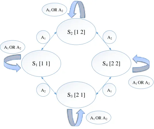
Figure 3-2: Possible state transitions in the insider trading problem ... 37

Figure 3-3: ε-greedy learning ... 41

Figure 3-4: Optimal learning ... 42

Figure 3-5: Boltzmann learning ... 44

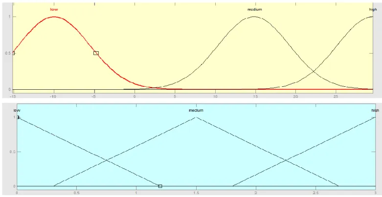
Figure 3-6: Quantile discretization ... 49

Figure 3-7: Single-input Mamdani fuzzy model membership functions and input-output curve ... 50

Figure 3-8: Output curve for Mamdani FIS ... 51

Figure 3-9: Fuzzy discretization ... 51

Figure 3-10: Sample Venn diagram ... 53

Figure 3-11: State transition diagram ... 55

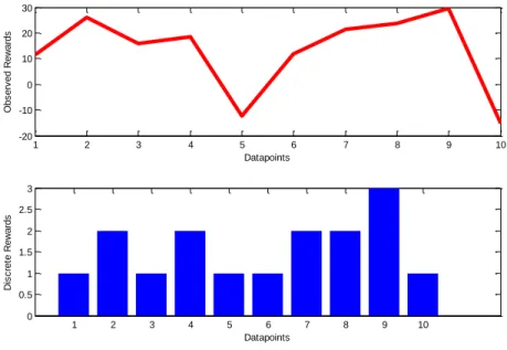
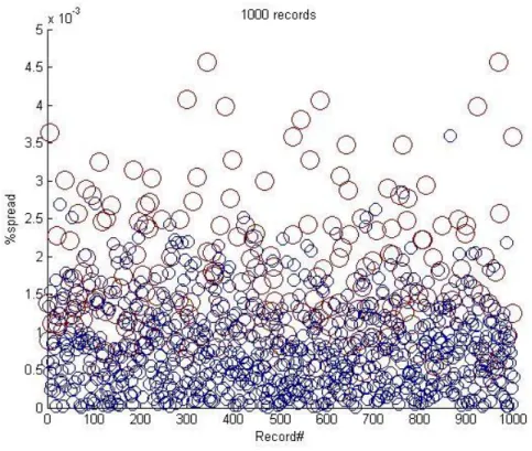
Figure 4-1: Insider trading reward distribution for a database of 1000 records. ... 67

Figure 4-2: Insider trading RL Search paths ... 68

Figure 4-3: Insider trading ROC for RL Search ... 69

Figure 4-4: Insider trading sensitivity rate for unsupervised algorithms across all testing percentages ... 71

Figure 4-5: Insider trading false positive rate for unsupervised algorithms across all testing percentages 72 Figure 4-6: Insider trading AUC for unsupervised algorithms across all testing percentages ... 73

Figure 4-7: Q-tables for training data ... 75

Figure 4-8: Q-table for validation on training data ... 76

Figure 4-9: Q-values for testing data. ... 76

Figure 4-10: Paths after discretization ... 77

Figure 4-11: Posterior probabilities for insider trading problem ... 78

Figure 4-12: State probability of risk for insider trading problem ... 78

Figure 4-13: ROC for supervised models insider trading ... 79

Figure 4-14: Insider trading AUC ... 80

Figure 4-15: Time difference variables distribution for deposit and withdrawal ... 82

Figure 4-16: DCFD RL Search Sensitivity ... 84

(11)

Figure 4-18: DCFD ROC for supervised models ... 87

Figure 4-19: DCFD AUC ... 87

Figure 4-20: CHHD RL Search Sensitivity ... 91

Figure 4-21: CHHD RL Search False Positive. ... 92

Figure 4-22: CHHD ROC for supervised models ... 93

Figure 4-23: CHHD state probabilities for supervised models ... 93

Figure 4-24: CHHD AUC ... 94

Figure 4-25: LFS RL Search Sensitivity ... 98

Figure 4-26: LFS RL Search False Positive ... 98

Figure 4-27: LFS ROC for supervised models ... 99

(12)

List of Tables

Table 2-1: Las Vegas Filter ... 22

Table 2-2: Confusion Matrix ... 26

Table 2-3: Example confusion matrix ... 27

Table 3-1: Records in a database ... 35

Table 3-2: States ... 35

Table 3-3: Link analysis using 4 records ... 37

Table 3-4: Q-table for insider trading problem ... 39

Table 3-5: Q-table for insider trading problem using ε-greedy learning ... 39

Table 3-6: V-table for insider trading problem using ε-greedy learning ... 39

Table 3-7: General search algorithm ... 40

Table 3-8: ε -greedy learning algorithm - general... 41

Table 3-9: Optimal learning algorithm ... 42

Table 3-10: Boltzmann learning algorithm ... 43

Table 3-11: Comparing learning algorithms ... 44

Table 3-12: V-table for the insider trading problem ε-greedy learning ... 45

Table 3-13: Optimal policy for all learning algorithms ... 46

Table 3-14: Probability of feature value occurring ... 53

Table 3-15: Probability of pairs of values occurring in the table ... 53

Table 3-16: State probabilities ... 54

Table 3-17: Transition probability calculations ... 57

Table 3-18: Transition probability matrix ... 58

Table 3-19: Empirical calculation of emissions matrix ... 58

Table 3-20: Solving HMM fundamental problems ... 58

Table 3-21: Hidden Markov Model procedure ... 60

Table 3-22: Classification steps ... 61

Table 4-1: Summary of database specifications ... 64

Table 4-2: Model summary and notation for thesis algorithms results. ... 64

Table 4-3: Insider trading characteristics of the data sets ... 66

Table 4-4: Unsupervised learning insider trading standard deviation (%) ... 74

Table 4-5: DB-PDF parameters for time difference model. ... 81

Table 4-6: DCFD statistics ... 83

Table 4-7: Unsupervised learning DCFD standard deviation (%). ... 86

(13)

Table 4-9: CHHD features ... 90

Table 4-10: Unsupervised learning CHHD standard deviation (%). ... 92

Table 4-11: LFS features ... 96

Table 4-12: LFS Database statistics – February 2013 ... 96

Table 4-13: Unsupervised learning DCFD standard deviation (%). ... 99

(14)

List of Acronyms

NN Artificial Neural Network

AUC Area under the ROC curve BAV Bellman Action-Value equation CHHD Canadian Heart Health Database CVD Cardiovascular disease

DB-PDF Double Bounded Probability Density Function DCFD Debit Card Fraud Database

EM Emissions matrix FICO Fair Isaac Corporation FIS Fuzzy inference system FN False Negative

FP False Positive

HyF RL-HMM hybrid with fuzzy discretization HyQ RL-HMM hybrid with quantile discretization HMM Hidden Markov Model

IC Inconsistency criterion

IIROC Investment Industry Regulatory Organization of Canada KNN K-Nearest Neighbour

LFS Labour Force Survey LR Linear Regression LVF Las Vegas Filter

MDP Markov Decision Process

NASDAQ National Association of Securities Dealers Automated Quotations RL Reinforcement Learning

RL-HMM Reinforcement Learning - Hidden Markov Model (hybrid) ROC Receiver Operator Characteristic

SMOTE Synthetic minority over-sampling technique SVM Support Vector Machine

TM Transition probability matrix

TN True Negative

TP True Positive

(15)

List of Variables

α Learning parameter in Bellman Action-Value equation 𝛼_𝑡(𝑖) forward probability variable

𝐴(𝑖) Number of actions available at state 𝑖 𝛽_𝑎𝑊 _{Precision of}_𝑊

𝑎

𝛽_𝑎𝑛 _{Precision update variable}

c Cut-off value representing the percentage of states classified as fraudulent 𝛿𝑚 Number of discrete values feature m is represented by in the database

ε Percentage of time policy explores the database (i.e. randomly select an action) 𝜆 Model parameter set in HMM

𝑃(𝑎) Probability of selecting action 𝑎 (for Boltzmann learning policy) 𝑝_𝑖𝑗 Probability of transitioning from state 𝑖 to state 𝑗

Φ Emissions probabilities in HMM 𝜋_𝑖 Initial state probability for state 𝑖

K Observation paths in HMM M Number of features in a database

N Number of states

O path of observable emissions Ω Finite set of γ types of observations Q Subset of states in HMM

𝑄(𝑖, 𝑎) Q-value for state-action pair (𝑖, 𝑎) in RL

𝑟_𝑖𝑗(𝑎) Reward in RL when agent moves from state 𝑖 to state 𝑗 by selecting action 𝑎 𝑆 finite set of 𝑁 states in HMM

𝜎_𝑊2_𝑎 _{variance of}_𝑊

𝑎 (for optimal learning policy)

𝑡 time

𝜏 temperature (for Boltzmann learning policy) 𝜃_𝑎𝑛 _{Estimate of}_𝜇

𝑎

𝜇_𝑎 mean of 𝑊𝑎

𝑉_𝜋 Optimal weights on each state in RL for policy π

𝑊_𝑎 Reward associated with RL action 𝑎 in the optimal learning policy 𝑋_𝑡 Random variable at time t

𝛾 Number of observations/emissions

(16)

Chapter 1 Introduction

Data mining of large databases has increased in societal importance as computers are faster, storage is larger and a large amount of data of varying data types is encountered. Generally, data mining is the search for patterns, behaviours and anomalies that cannot be easily calculated from the data or gleaned from a visual representation.

Databases in industry generated by human behaviour often may have examples that reflect an exchange of risk for reward, for example, financial market trading. Risk may be both a qualitative and quantitative measurement of what someone is willing to sacrifice for a potential reward [ [1], [2], [3]]. High risk is usually associated with high rewards. An example of a risk-reward system is a financial market in which the corresponding risky behaviour is insider trading. Health is another example of a system in which there is a risk-reward relationship associated with lifestyle characteristics such as high stress and poor diet [4]. A paradigm shift in the approach to data mining of risk-reward systems is introduced in this thesis by modeling, isolating and exploiting two types of risky human behaviour: collusion and repeated abuse. Collusion is a secret agreement between two or more persons for a deceitful or illegal purpose [5]. This definition is extrapolated to be “two or more database features” for a “risky” purpose where a “feature” is a column in the dataset. A recent example of collusion in finance is in the foreign exchange markets where traders at different leading global financial institutions colluded to manipulate benchmark foreign exchange rates between 2009 and 2012 [6].

Repeated abuse occurs when consistently higher than average rewards are associated with risky activity. “Abuse” is a term known to be associated with taking advantage of a system, such as finance or the human body.

A general exploration of collusion and repeated abuse has not been previously researched in data mining literature and is the foundation of this thesis [7]. In addition to a lack of modeling general behaviours in risk-reward systems, current data mining solutions are limited by unadaptive solutions [8], domain-centric models [7], a lack of knowledge-based components [8] as well as lack of focus on misclassification [7]. In the following sections, the risk-reward problem will be described in the context of data mining as well as the representative learning and decision-making models. Performance evaluation and the need for algorithm design to meet the needs of industry are also discussed. In the last section the thesis outline will be presented.

(17)

1.1 Problem Description

The main objective of most data mining applications is to accurately identify specified samples in the dataset. The objective of this research is to detect risky behaviour with a classifier. The classifier is evaluated based on its ability to find the risky samples (called sensitivity or recall) and misclassify non-risky samples as non-risky (called false positive). The datasets are primarily bi-class imbalanced; these are datasets in which there are two classes and the majority class (non-risk) is much larger than the minority class (risk). Ultimately the problem is to construct the most sensitive classifier with the lowest

misclassification rate, not necessarily the most accurate classifier. The problem of characterizing risky behavior is approached using machine learning algorithms and statistical models.

1.1.1 Description of risk – reward relationship for data mining

Risky behaviour in risk-reward systems is modeled by feature values in the database sample

corresponding to high rewards. The features are types of “behaviour” and the reward is a feature in the database summing up the benefit of that behaviour. Collusion and repeated abuse are represented by several samples having the same feature values corresponding to high rewards. In specific scenarios, high rewards can be associated with smart investing, or healthy living, for example. It is assumed that cases such as these do not exhibit the same feature values in all samples whereas risky samples in the thesis applications do share feature values.

1.1.2 Learning and decision making

To learn is to acquire knowledge, understanding, or mastery (of) by study, or experience [9]. Learning to solve a problem requires decision-making: selecting the optimal steps to reach a solution.

Machine learning has been employed by data miners across many industries to solve problems such as forecasting consumer behaviour (retail [10], online advertising [11]), and anomaly detection (health [4], finance [7] [12]). In this thesis, machine learning is used to learn the behaviour of the risky person through experience. The learning process consists of an “agent” making decisions as it explores the database to derive optimal decisions for achieving the highest rewards. Machine learning algorithms are known to require a lot of experience to draw conclusions [13]; this means they use a lot of data and time. To minimize this aspect, a statistical model was integrated with the optimal behaviour paths to uncover the samples with groups of feature values resulting in the highest rewards.

1.1.3 Classification of imbalanced databases

“Bi-class” or “binary” classification problems can be considered as anomaly detection problems, particularly in imbalanced databases [14]. For the purpose of binary classification, risky samples are

(18)

labeled as “positive” and non-risky samples as “negative”. Because of the imbalanced distribution of the classes, traditional classifiers can easily find the negative class because there are so many samples to use for modeling. These classifiers do not describe the positive class data at all and usually consider it as part of the negative class. This results in high misclassification costs, which are unacceptable in industrial applications [15]. Approaches to the problem manifest in three ways: data level techniques to balance the data, algorithm techniques which model the minority class, cost-sensitive methods that combine data and algorithm techniques by assigning misclassification costs to classes [15]. He and Garcia [16] describe the objective of classification for imbalanced data is to obtain high accuracy for the minority class while not jeopardizing the accuracy of the majority class. Therefore, an algorithm technique is used in this thesis to solve the problem. It is evaluated by specific metrics to reflect the ability of the classifier to identify the minority class. This objective is further explored in the thesis.

1.1. Research objectives and scope

The objective of this research is to accurately represent the risky behavioural patterns of agents in risk-reward systems. The problem is approached by constructing three models: an unsupervised

Reinforcement Learning Search model, a Reinforcement Learning Classifier and a hybridized classifier using a Reinforcement Learning algorithm and a Hidden Markov Model. To capture the agents’ risky behaviour three learning algorithms are employed: ε-greedy, Optimal Learning, and Boltzmann learning. The classifier is evaluated on four real-world databases, one of which contains balanced classes to test its applicability outside of anomaly detection problems. Ultimately, the intention is to integrate the model into an industrial system; the goal is achieved when a sensitive classifier is constructed with minimal misclassification.

1.2. Thesis outline

The requisite background knowledge and a general literature review of relevant research on machine learning and statistical models in the context of data mining are presented in Chapter 2. In Chapter 3, the Reinforcement Learning algorithms and Hidden Markov Model formulations are proposed. The methods are then applied to financial fraud, heart disease, and female labour force participation in Chapter 4. The conclusions and contributions to knowledge are summarized in Chapter 5.

(19)

Chapter 2 Background and Literature Review

2.1 Introduction

The exciting problem of representing risky behavioural patterns of humans in risk-reward systems is best understood contextually. Collusive and repeatedly abusive behaviour are known to be systemic in financial fraud and are both manifestations of “greed” [17]. The research conducted here was motivated by the author witnessing such behaviour for insider trading while working at a bank. The specific type of insider trading observed is called “front running”, the practice of manipulating rates on a client's order to skim off extra points for the bank. Manipulation usually involves some knowledge of future trades (e.g. insider information) to know the direction of the market. This type of financial fraud can be collusive and frequently involves repeated abuse; a trader who is willing to front run one client is likely willing to front run many clients. Front running is the main lever Bernie Madoff used [18] [19] to execute his Ponzi scheme in the years preceding the Global Financial Crisis of 2008; it is a common practice in the financial markets regulated in the equity and derivative markets by IIROC [20] in Canada. One of the chief

investigators of the Madoff case, Harry Markopolos, claims that front running is a widely occurring, common abuse that is openly tolerated [19] but has widespread consequences. It is therefore necessary to characterize and identify this behaviour in the trading book so as to prevent and minimize the damage to investors and the financial markets.

Palshikar and Apte [21] approached collusion detection using a graph-clustering algorithm, playing on the “network” aspect of collusion sets. Their work inspired Wu et al [22] to focus on one type of collusion-based financial crime – circular trading in stock markets. This is a practice of colluders (called a

“collusion set”) circulating a large amount of shares within a short period of time to feign demand for the stock. They approached the problem using a standard HMM with the Nelder-Mead simplex method for parameter estimation. The term "collusion" appears [19] several times in descriptions of fraudulent scenarios where multiple participants perpetuated fraud. The manipulation of foreign exchange [6] and interest rates [23] are examples of collusive behaviour for which legal proceedings are in progress for traders at several banks colluding over instant messaging to manipulate rates for profit.

More generally, insider trading is a crime for which systems have been constructed for detection. In the American stock exchange, NASDAQ [24], the problem of insider trading is attacked by reviewing market activity for stocks that will have material news released that day by the stock-issuing company [25]. Their treatment of insider trading is focused on trading that occurs on material non-public information. The main limitation is that the system is not flexible for new domains or markets and requires a lot of maintenance due to its level of detail. Other fraud detection systems rely on scenarios of events

(20)

(time-based) and known patterns [8]. The scenarios and patterns are updated after consultation with domain experts, a detection paradigm that lacks automated adaptability.

On a larger scale, financial fraud is a pervasive practice ranging from mortgage fraud to accounting fraud, money laundering to insider trading [7]. This research focuses on two types of financial fraud: insider trading (including front running), and plastic card fraud (debit card fraud). Lu states two challenges to fraud research [26]: 1) secrecy with regards to techniques - banks do not want people to know their techniques so the public can get around them, 2) limited availability of real fraud records. These challenges were overcome by accessing public information and using techniques gleaned from the author's work experience in the financial industry.

The authors of [27] comment that the major task in fraud detection is the construction of algorithms or models that can learn how to recognize a variety of patterns [27]. While collusion and repeated abuse can be viewed as two patterns, they cover a large behavioural space and generalize a lot of patterns. They are also not content specific and, within an adaptable system, can classify many types of behaviour under one umbrella.

Zhang and Zhou [27] emphasized that fraud detectors require systems that can detect rare events, outliers or noise. There is evidence that financial fraud is often executed by the same individual repeatedly via transactions in which he is making higher than normal profits [17]. Traders are aware that sophisticated algorithms exist to detect their transactions. Therefore, the risk of being detected is lower when trades are slightly more profitable than average trades as opposed to executing extremely profitable trades.

Repeated abuse can be characterized by frequency and density. Plastic card fraud experiences this phenomenon where several transactions are executed rapidly and in nearby locations. A systems diagram of a typical industrial financial fraud detection system with inputs and outputs is shown in Figure 2-1.

Figure 2-1: Financial fraud detection systems diagram

Financial transactions are the raw data that is preprocessed, grouped and classified based on the System Model used by the financial institution. Examples of the System Model are Linear Regression, Artificial Neural Networks, and Rule-based systems [7]. The resulting patterns are compared to known patterns

System Model Known patterns

Fraudulent transaction

ID Financial

(21)

and those that either match known patterns of fraud or do not match regular patterns of behaviour are output as fraudulent transactions or “breaks” [28]. These breaks are not necessarily descriptive. The entire transaction is visible, but the reasons for which it was flagged are because it broke a rule or was anomalous to known behaviour. Since the fraud detection is conducted on a one-off basis, seemingly fair transactions go undetected. However, when several “fair” transactions are grouped together by an individual or asset, the behaviour can be illegal. Therefore, current industrial methods are not focused on detecting groups of fraudulent behaviour such as those modeled in this thesis.

In [19], Francis suggests that financial regulators must act like public health experts and constantly search for pathologies (e.g. criminal pathologies) that have the capacity to spread and cause severe crisis. The health analogy of pathology of financial fraud allowed us to consider general systems that demonstrate risky pathologies.

Financial systems are generalized as “risk-reward” systems because humans acting on the system absorb some level of risk for reward. This system representation can then be extended to other systems in which risk is exchanged for reward. An example of such a system is the human body. Humans make risky decisions with respect to their lifestyle choices in exchange for heart disease. Conversely, a non-risky (healthy) lifestyle is typically rewarded with long life. Repeated abuse is a characteristic of human systems where poor choices are made daily. Additionally, different choices can collude in the human body with deleterious results [4]. Dahlof observed that moderate risk levels in several risk factors is often more dangerous to health than large risk in one risk factor. Heart disease is commonly detected by

searching clinical data where there are more cases of health than disease.

Diagnosis of heart disease has been approached from a risk perspective in the literature [29] [30]. The authors remark that in the emergency room, clinicians require a decision-making tool to assess risk and diagnosis. Liu et al [30] use a combination of data level sampling processed through an ensemble of support vector machine classifiers (SVM) from which a risk score is generated. They simulate the real-world medical setting where more than one opinion is sought before making final decisions.

Heart disease has been generalized in this research to a “risk-reward” system based on the literature and that it is related to “risky behaviour”. Health is certainly a more complicated domain with underlying genetic and biological systems that we cannot necessarily control nor fully understand. In the interest of studying imbalanced databases we pursued heart disease with the understanding that a domain expert would be required in order to accomplish a more thorough investigation in the health care domain. In the context of data mining, isolating cases of collusion and repeated abuse can be a classification problem: from a group of samples, a subset is classified as risky, and the rest of the samples are classified as non-risky. This can also be considered as an anomaly detection problem in which the model figures out or is instructed as to what is “normal” behaviour, and then uses a distance calculation to compare new

(22)

samples to “normal” samples. The main problem with an anomaly approach is that suspicious samples are dependent on described normal or average behaviour in the database, and anything else is labeled fraud.

Many different algorithms have been developed to solve the problem of fraud detection, and more generally, classification: linear regression (LR), artificial neural networks (NN), support vector machines (SVM), and K-nearest neighbor (KNN). Because classification is a broad area, the following literature review is performed only on some of the methods related to fraud detection and generally, imbalanced databases. Imbalanced databases have many more samples belonging to some classes than others whereas balanced databases have a consistent number of samples attributed to each class. A deeper discussion of imbalanced databases will follow later in Chapter 2. The literature review will also discuss Reinforcement Learning and Hidden Markov Models which were used to develop new methods for classification of imbalanced databases in the thesis. The sections in this chapter will present detailed background information on relevant concepts and mathematical formulations popular in the literature.

2.2 Important Reinforcement Learning concepts and techniques

Reinforcement Learning (RL) is a computational approach to learning from interaction between an agent and its environment [31]. It is a type of goal-directed learning in which the agent receives a numerical reward signal. RL is model-free; it does not fit the data to a function nor estimate function parameters. In practice, this means that it does not require a transition probability matrix as in a Markov Decision Process (MDP) [32]. It simply begins searching through the environment without any examples of desired behaviour by making decisions and assigning scores to each example of behaviour [33]. The study of behaviour dates back to 1911 in which Thorndike [34] studied animal psychology. He concluded that animals learn from experience and associations, not memory or imitation. In particular, repetition of an experience consecrates a reaction in the animal’s mind to reach a goal. RL applies the concept of repetition by frequently visiting states of the system that provide the highest reward.

RL is classically applied in the field of control theory where actions are repeated and modified until stability or an optimal policy is achieved [33] [13]. The applications range from manufacturing to playing games to optimal routing [35]. RL appeared in the data mining literature as part of a Learning Classifier System in 1978 but gained popularity in the early 1990s [36]. Since then, RL has been applied to classification [37] [38], clustering [39] [40], and outlier detection problems [41].

The application of RL in this thesis was motivated by financial fraud investigative techniques used by Lu [41]. Lu's exploration of fraud detection hinged off constructing a “fraud case builder”. The goal of the algorithm was not to find fraud; instead it was to gather the elements contributing to fraud, and build policies that dictate fraudulent behaviour. RL is an improvement to current systems by performing the

(23)

role of identifying suspicious data. Due to its “trial and error” approach, it eliminated the need for expert intervention because it built a body of evidence based on best rewards [42]. Sawh et al. [43] applied RL to two problems in finance: derivation of an optimal trading strategy and detection of insider trading. Lu [41] and Sawh et al. [43] demonstrated how operating in a model-free environment increased the agent’s ability to detect new instances of anomalous data. RL does not require knowledge of the entire

environment; calculations are based on a temporal differencing equation which only looks one step ahead. This is in contrast to learning models that examine an entire database or network [44]. RL examines data directly by linking records with large rewards; other learning methods often group records based on statistical features [45]. The main disadvantage of RL is that sometimes the problem can have a large state space; it takes a long time to converge and requires a lot of data to learn the problem [33] [46]. The ability to operate unconstrained can be a disadvantage because it might identify anomalies that do not characterize anomalous behaviour and draw incorrect conclusions. Improvement to RL techniques will be presented later in this thesis.

2.2.1 Reinforcement Learning components

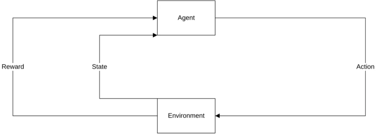
The RL problem is described by three main components: an agent, an environment and an action. In engineering terms, the components are analogous to a controller, a controlled system/plant and a control signal. A schematic of the components is shown in Figure 2-2.

Figure 2-2: Component diagram of agent-environment interaction

The agent interacts with the environment by an action. Once the action is taken, the environment produces a numerical reward. The agent receives the information, evaluates it and selects an action based on the evaluation. The action takes the agent to the next state. In defining an environment, anything that cannot be changed arbitrarily by the agent is considered to be part of the environment.

Generally, states are the information available to the agent, actions are any decision it wants to learn how to make, and rewards represent desired outcomes. For example, if the system problem is a human

Agent

Environment

Action

(24)

throwing a ball, then the states are the different positions of the human muscles in the act of throwing. The action is throwing the ball and the reward is the accuracy of the throw.

The difference between MDPs and RL is that RL does not require transition probabilities to move between states; rather, change of state is dictated by action selection. A reward function is also not required by RL. Instead, the reward is computed and collected as the agent traverses the environment. An important step in RL is that the agent must collect a reward before recognizing a new state as part of the feedback loop. In the example of throwing a ball, a human must assess the accuracy of his throw before throwing again. In doing so, he can modify his eye-hand coordination and muscle movement so that the next throw is more accurate. In the sport of baseball, athletes repeatedly throw balls to train their muscles during practice so that they do so automatically and accurately under the pressure of a game.

2.2.2 Bellman Action-Value equation

RL applies a temporal differencing method called the Bellman Action-Value equation (BAV) [31] for solving MDPs:

𝑄𝑡_{(𝑖, 𝑎) = 𝑄}𝑡_{(𝑖, 𝑎) + 𝛼[𝑟}

𝑖𝑗𝑡(𝑎) + 𝛾𝑄𝑡(𝑗, 𝑏) − 𝑄𝑡(𝑖, 𝑎)] (2-1) In the BAV equation (2-1), 𝑖, 𝑗 are the states, 𝑎, 𝑏 are actions, and 𝑟_𝑖𝑗(𝑎) is the reward obtained when the agent moves from state 𝑖 to state 𝑗 via action 𝑎. The equation also supplies a learning rate, α, which controls the rate of convergence of the model. RL methods can be episodic or continuous. For episodic applications, the discounting factor 𝛾 = 1 because the applications do not require discounting in time. All applications in this thesis were episodic. The symbol for time, 𝑡, represents the simulation number and if the RL algorithm is run over the input table 100 times, then t = 1, … ,100.

The agent begins at state 𝑖 and takes action 𝑎. The agent's position is represented by a “state-action” pair, (𝑖, 𝑎). The agent then obtains a new state-action pair, (𝑗, 𝑏), from where the next iteration will begin. The resulting values output from equation (2-1) are called “Q-values”. Q-values are stored in a matrix called a “Q-table” where each cell represents a value for 𝑄(𝑖, 𝑎). The matrix is of size (number of states x number of actions). Q-values are considered to be “weightings” on each state-action pair.

Once the simulation has converged and the Q-table is complete, the optimal action (i.e. decision) is determined for each state. This translates into the optimal behaviour of the agent in each state. To do this, the heaviest weightings for each state are examined. The corresponding actions are the underlying behaviour to be extracted and studied. Therefore the maximum Q-value is selected for each state. The resulting column vector of states is called the “V-table”.

The V-table represents the “optimal policy”. A policy is a stochastic rule by which the agent selects actions as a function of states [31]. The optimal policy maps the best action for each state. The best action

(25)

represents the action that returns the highest reward in that state. The agent's objective is to maximize the amount of reward it achieves over time. The V-table gives the maximum return across all actions for each state.

Knowledge of the optimal policy is useful to decision-makers in three significant ways. It indicates what action to take, in the future, when in that state. It indicates the action resulting in the highest reward for each state. In a reverse engineering problem it indicates the optimal path of states and actions for the environment.

Temporal differencing is appropriate for data mining applications because it links records in a database. By differencing between two Q-values in equation (2-1), it finds a differential, or a distance in Q-values. The size of this difference contributes to the Q-value, and ultimately, the weighting of that state. For those states that are close in weights, the Q-value is smaller and thus the state-action pair is similar to the other state-action pairs. However, when the Q-values greatly differ, the larger Q-values represent a deviating state-action pair. Over many simulations one state-action pair is compared with several others and a distinct set of state-action pairs stand out as significantly weighted.

2.3 Learning algorithms

In Reinforcement Learning optimal policies are used to take actions. These policies are constructed by learning algorithms. The learning algorithms “learn” the problem by balancing between exploration and exploitation. Exploration of the database occurs when the learning agent varies the actions it takes in order to explore opportunities for finding higher rewards. This behaviour is equivalent to a non-risky human who varies his decisions according to the environment. Exploration also allows the agent to search for collusive agents in the database. Exploitation occurs when the learning agent has found the action that consistently returns higher rewards and repeatedly takes that action in order to achieve the highest expected value. This is the behaviour of a risky agent who repeatedly abuses a system. The behaviour of the decision-makers must be learned based on the assumption that risky human

behaviour is adaptive; in this sense the learning agent is “unsupervised” in that it is not told which state to go to and does not realize a reward until it reaches that state. RL is an unsupervised model when it is not trained on data containing the true classes (i.e. labeled data). When the agent is exposed to true class labels during the learning process it is “supervised” because it is trained on labeled data. The models in this thesis use RL in both its unsupervised and supervised forms.

There are four common policies in the literature: random, greedy, ε-greedy and Softmax [31]. The random policy is purely exploration; there is no preferred action. Therefore the probability of selecting an action is _|𝐴(𝑖)|1 where |𝐴(𝑖)| represents the number of actions available at state 𝑖. The random policy is

(26)

called Sarsa in the literature [31]. Sarsa stands for: State, Action, Reward, State, Action. It tends to be exploratory and time-consuming.

The greedy policy is a purely exploitative learning algorithm, called Q-learning. Because action 𝑎 has the highest Q-value for state 𝑖 and is selected each time the state is visited, 𝑄(𝑖, 𝑎) increases and therefore the same action is selected each time. Q-learning is an exploitative method that follows the greedy behavior. Q-learning is considered to be an “off-policy” method because it is always maximizing(𝑖, 𝑎)∀ 𝑎 ∈ 𝐴(𝑖). Therefore the policy for action selection is not “learned”; it is the same every time.

The ε-greedy policy balances exploration and exploitation based on the value of ε. Actions in the set of admissible actions are selected with probability _|𝐴(𝑖)|𝜖 . The Softmax policy, also known as Boltzmann Learning [47] is another method of balancing exploration with exploitation. The probability of selecting an action is given by the following formula:

𝑃(𝑎) = 𝑒𝑄(𝑖,𝑎)/𝜏 ∑ 𝑒𝑄(𝑖,𝑧)/𝜏

𝑧∈|𝐴(𝑖)| (2-2)

where 𝑄(𝑖, 𝑎) is the action-values for state 𝑖 when action 𝑎 is taken. 𝜏 is a positive number called

temperature which is the variable used for tuning the model to the problem. When the temperature is high the probabilities of taking all actions are the same; as the temperature decreases with the number of samples, the higher probabilities are assigned to actions with higher values for 𝑄(𝑖, 𝑎). This results in an exponentially increasing probability for the most frequently selected action. Boltzmann learning has the advantage of not spending a lot of time on bad alternatives and works best when there are a small number of alternatives (e.g. less than 100) [47].

The third learning algorithm employed in this thesis is a statistical method outside of the RL literature; it is called “Adaptive learning” [47]. This is a novel approach to learning in the RL setting introduced by this thesis. In honour of Powell’s text this learning algorithm will be called “optimal learning” going forward. Optimal learning is set in a Bayesian framework; the Bayesian perspective is primarily

interested in estimating the mean and variance of µ which is the true mean of the random variable W. In the RL setting, the random variable W represents the reward associated with a RL action and is recast as 𝑊_𝑎. The model assumes that a prior distribution of belief about the unknown parameter 𝜇_𝑎 exists and that selection of one action over another is independent.

The action with the highest estimated mean reward is selected when the agent enters a state. The mean for the action selected is updated with the reward the agent collects.

It is assumed 𝑊𝑎~𝑁(𝜇𝑎, 𝜎𝑊𝑎 2 ₎_._𝜃

𝑎𝑛 is used to estimate 𝜇𝑎 after n observations for action a. 𝛽𝑎𝑛 is used to estimate the precision of 𝑊_𝑎 as 𝛽_𝑎𝑊=_𝜎1

𝑊𝑎2 . 𝜃_𝑎𝑛_{is iteratively updated using equation (2-3):}

(27)

𝜃𝑎𝑛+1 =

𝛽_𝑎𝑛_𝜃

𝑎𝑛+ 𝛽𝑎𝑊𝑊𝑛+1

𝛽_𝑎𝑛_{+ 𝛽}

𝑎𝑊 (2-3)

𝛽_𝑎𝑛_{is iteratively updated using equation (2-4):}

𝛽_𝑎𝑛+1_{= 𝛽}

𝑎𝑛+ 𝛽𝑎𝑊 (2-4)

Once the agent collects a reward Wn+1 is set equal to the reward which represents the newest information in the model. The equations for 𝜃𝑎𝑛 and 𝛽𝑎𝑛are then updated for each action. Then the action producing the highest mean is selected: max_𝑎∈𝐴𝜃_𝑎𝑛.

The learning algorithms presented in this section were selected based on their diversity; varying from simple to complex, and a mix of artificial intelligence with statistical methods. Moreover, they most similarly mimicked a risky agent in a risk-reward system by repeatedly abusing the system (i.e. exploitation) while colluding with other agents (i.e. exploration).

The RL algorithm finds the optimal path of a risky agent. The path outputs are Q-values and rewards. This research used Q-values to determine risk in the RL Search and RL Classifier models. To assess state riskiness using rewards, a Hidden Markov Model was applied.

2.4 Important Hidden Markov Model concepts and techniques

The intuition behind Markov models is to use the Markov property to simplify a Markov chain of events. 𝑃[𝑋_𝑡+1|𝑋_𝑡, 𝑋_𝑡−1, 𝑋_𝑡−2, … , 𝑋₀] = 𝑃[𝑋𝑡+1|𝑋𝑡] (2-5) (2-5) says that the value of 𝑋_𝑡 in the next time step is only determined by the most recent value of 𝑋_𝑡 and not the entire set of values 𝑋_𝑡 has taken in the past [48].

In practice, this means treating a stochastic process {𝑋_𝑡|𝑡 ∈ 𝑇} as a first-order Markov process. Typical Markov model analysis assumes that the state sequence of the process is known and observable. In a Hidden Markov Model (HMM), the state sequence through which the process passes is unobservable. The objective of the HMM is to use a sequence of observations of the dynamics of the process to uncover the underlying hidden states [32].

Formally, a HMM is applied when the problem is to recover a sequence of states 𝑥(𝑡) from observed data 𝑦(𝑡). The main assumption is that a Markov chain is the underlying process with internal states hidden from the observer [32]. HMM solves the conditional probability in equation (2-6).

𝑃[𝑦(𝑡)|𝑥(𝑡)] (2-6)

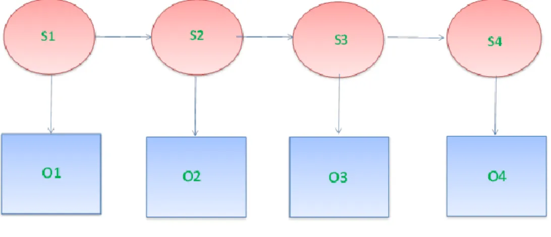
The observations are the output of the system, and are also referred to as “emissions”. HMMs are applied to state-based systems where the system outputs an emission when it arrives in a state. There are a finite number of possible emissions and states.

(28)

Hidden Markov Models are doubly stochastic processes. According to Ibe [32], this means that an underlying stochastic process is unobservable and can only be observed through another stochastic process that produces a sequence of observations. Using one observed stochastic process to derive another stochastic process makes it a doubly stochastic process. Figure 2-3 shows the two processes and the link between the states that make them sequential.

Figure 2-3: HMM representation

The square boxes represent the emissions O1, O2, O3, O4 that are some observable output from the system. These observations relate to hidden states S1, S2, S3, S4. The goal of a HMM is to find the states, in the correct order, that produced the emissions. The state sequence is found based on the information stored in two matrices: a transition matrix, 𝑃[𝑥(𝑡 + 1)|𝑥(𝑡)] which describes the probability of an agent’s transitions between states and an emissions matrix, 𝑃[𝑦(𝑡)|𝑥(𝑡)], which describes the probability of the output given the current state.

HMMs have many applications, the most popular being in speech recognition [49]. The observed data in this case is sounds and the hidden states represent words. The application of HMM in this thesis was motivated by Eisler’s application of HMM to uncover financial market volatility [50]. Volatility measures the uncertainty about returns of a stock [1] which is not directly observable from the stock prices

themselves. Volatility is instrumental in the decisions made by financial market agents because it gives the perception of the risk associated with that stock [51]. Eisler et al. selected HMM so they could visualize the sample path taken by volatility over time. The research by this thesis is intended to uncover risky behaviour, a hidden process like volatility.

HMMs appear in the financial fraud literature as well. Wu et al [22] observed financial trades to uncover multi-variable states where the variables indicate whether a transaction is malicious and part of a

collusion set. Khan et al [52] used HMMs to uncover spending behaviour via observed credit card transactions.

(29)

1. To derive the sequence of states, indexed by time, from a set of observations. 2. To assign probabilities of classes in the test dataset.

The main disadvantage of HMM is that model training can take long and convergence is not guaranteed [32]. The model is constrained by probabilistic assumptions which can be too restrictive for some systems. The documented limitations were overcome in this research by training the model using RL and then applying the HMM probabilistic model assumptions to quickly derive risky states.

2.4.1 HMM components

In a HMM model with N states, γ emissions and 𝑡 = {1, 2,3, … , T} steps in a sequence, the fundamental variables are as follows:

𝑆: finite set of N states 𝑆 = {𝑠1, 𝑠2, 𝑠3, … , 𝑠𝑁}

Ω : finite set of 𝛾 types of observations Ω = {Ω1, Ω2, Ω3, … , Ω𝛾}

𝑄 : hidden states 𝑄 = {𝑞1, 𝑞2, 𝑞3, … , 𝑞T}

O: path of observable emissions 𝑂 = {𝑜1, 𝑜2, 𝑜3, … , 𝑜T}

𝑄 is a subset of 𝑆

K : observation paths 𝐾 = {𝑘1, k2, k3, … , 𝑘𝐾}

𝑆 is a hidden Markov process that is observed through Ω; therefore Ω = 𝑓(𝑆) for some function 𝑓. 𝑆 is the state process and Ω is the observation process. The model parameters calculated prior to solving the HMM are the transition probabilities (𝑃 = {𝑝_𝑖𝑗}), emissions probabilities (Φ = {𝜙_𝑖(𝑜_𝑇)}) and initial state probabilities (𝜋 = {𝜋_𝑖}); When describing an HMM it is customary to denote the triplet 𝜆 = (𝑃, Φ, 𝜋) for the model parameters used to fully define the model.

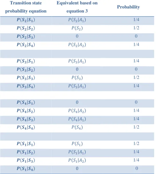
The transition probabilities 𝑃 = {𝑝_𝑖𝑗} reflect the probability of moving from state 𝑖 to state 𝑗 in a discrete first-order Markov chain. The Markov equation for transitioning between states is given by,

𝑃(𝑞_𝑡+1 = 𝑗|𝑞_𝑡 = 𝑖, 𝑞_𝑡−1= 𝑙, 𝑞_𝑡−2= 𝑚, … , 𝑞₀ = 𝑛) = 𝑃(𝑞_𝑡+1= 𝑗|𝑞_𝑡 = 𝑖) = 𝑝_𝑖𝑗, (2-7)

describing the assumption that the future state depends only on the current state. The probabilities satisfy conditions 1 and 2 [32]:

1. 0 ≤ 𝑝𝑖𝑗 ≤ 1

2. ∑ 𝑝𝑗 𝑖𝑗 = 1, 𝑖 = 1,2, … , 𝑁, since the states are mutually exclusive and collectively exhaustive. They are displayed in an [N x N] matrix 𝑃 which will also be called a “transition probability matrix” (TM) in this thesis. It takes the form:

𝑃 = [

𝑝₁₁ ⋯ 𝑝_1𝑁

⋮ ⋱ ⋮

(30)

The TM models the transitions between states thereby giving a fully-defined space from which to derive a state sequence.

A state transition diagram is a graphical representation of 𝑃. One is shown in Chapter 3 describing the fundamental transition assumptions underlying the algorithms developed during this research. Another component of 𝜆 is Φ = {𝜙_𝑖(𝑜_𝑇)}, the emissions matrix (EM). It is an [N x γ] matrix mapping the probability of an observation given that the system is in a specific state.

𝜙_𝑖 = 𝑃(𝑜_𝑡|𝑆𝑖) (2-8)

The EM can be calculated using two methods:

1. Empirical method. The probabilities are derived from observations resulting from some dynamic process which transitions through states in sample data.

2. Theoretical method. The probabilities are derived from a probability distribution of expected observations when in each state.

Note that the rows of the EM sum to 1. This is because the total probability of state output emissions must equal 1.

The final component of λ are the initial state probabilities, 𝜋 = {𝜋_𝑖}, otherwise known as the marginal probabilities. 𝜋𝑖 describes the probability of a single event occurring. A joint probability is the probability that two events will occur simultaneously. 𝑝𝑖𝑗 is a joint probability because it gives the probability of an agent being in 𝑠𝑖 and going to 𝑠𝑗. The marginal probability describes the probability that the system is in 𝑠𝑖, not accounting for where it transitioned to or from, and is used as the initial

probability for state 𝑠𝑖 of the system.

The system of equations represented by 𝐴𝑥 = 𝑏 is used to solve for π. 𝐴 = 𝑃 with the last row of 𝑃 replaced with 1s to satisfy the sum of probability condition [53]. 𝑥 is a vector of 𝑁 marginal probabilities and 𝑏 = [0,0, … 1].

The resulting probability output from the HMM is a posterior state probability. It is the conditional probability of being at a state given an observation and model λ.

𝑃(𝑄|𝑂, 𝜆) (2-9)

This calculation results in a [N x 𝛾] matrix. Posterior probabilities condition on observations so the total probability for the observation is distributed among the states. The columns of a posterior probability matrix sum to 1.

2.4.2 HMM assumptions

(31)

1. Markov Assumption

The next state in a system depends only on the current state, and the transition probabilities are defined by equation (2-7). The HMM is first-order.

2. The stationarity assumption

The state-transition probabilities are independent of the actual time the transitions take place. Thus, for any two times 𝑡1 and 𝑡2,

𝑃(𝑞𝑡1+1= 𝑗|𝑞𝑡1= 𝑖)) = 𝑃(𝑞𝑡2+1= 𝑗|𝑞𝑡2= 𝑖, ) = 𝑝𝑖𝑗 (2-10) 3. The observation independence assumption

The current observation or output is statistically independent of previous observations.

2.4.3 HMM fundamental problems

There are three fundamental problems that can be solved using HMM:

1. The learning problem. Given a set of observation sequences find a HMM that best explains the observation sequence. Find 𝜆∗= 𝑎𝑟𝑔𝑚𝑎𝑥𝜆𝑃(𝑂|𝜆).

2. Evaluation problem. Given a model 𝜆 = (𝑃, Φ, 𝜋), find the probability that observation sequence 𝑂 = {𝑜1, 𝑜2, 𝑜3, … , 𝑜T} comes from that model. Find 𝑃(𝑂|𝜆).

3. Decoding problem. Given a model, 𝜆 = (𝑃, Φ, 𝜋), find the most likely sequence of hidden states that could have generated a given observation sequence. Find 𝑄∗= 𝑎𝑟𝑔𝑚𝑎𝑥_𝑄𝑃(𝑄, 𝑂|𝜆). The learning problem estimates the HMM parameters 𝑃, Φ, 𝜋 given a set of observations in a training set. The Baum-Welch algorithm is commonly used to solve this problem [32]. In this thesis, HMM

parameters are calculated empirically from the observations collected by the RL agent, a procedure described in Chapter 3. The Baum-Welch algorithm is not used.

The goal of solving the evaluation problem is to find 𝑃(𝑂|𝜆). The evaluation problem estimates the probability of an emission 𝑜_𝑡 given the model 𝜆 = (𝑃, Φ, 𝜋). The most straightforward way to find this probability is to enumerate all possible state sequences of length T and then sum their output probabilities [54]. The method forms a trellis of states and calculates the probability of each state occurring at a specific time in the sequence, 𝑡_𝑖. [32]. For the calculation, compute a forward probability variable 𝛼_𝑡(𝑖) as defined in equation (2-11).

𝛼_𝑡(𝑖) = 𝑃(𝑜1, 𝑜2, … . , 𝑜𝑡, 𝑞𝑡 = 𝑠𝑖|𝜆)𝑡 = 1, … , 𝑇; 𝑖 = 1, … , 𝑁 (2-11)

𝛼_𝑡(𝑖) represents the probability of being in state 𝑠_𝑖 at time 𝑡 after having observed sequence

{𝑜₁, 𝑜₂, … , 𝑜_𝑇} . It is calculated by summing probabilities for all incoming arcs in the trellis node. The forward algorithm is implemented by the following steps:

(32)

Initialization:

𝛼₁(𝑖) = 𝜋𝑖 𝜙𝑖(𝑜1) 1 ≤ 𝑖 ≤ 𝑁 (2-12)

In the initialization step, the forward probability variable for state i is calculated as the marginal probability for state i multiplied by the emission probability of observation 1 (𝑜1) coming from state i. Induction:

𝛼_𝑡+1(𝑗) = {∑ 𝑝_𝑖𝑗

𝑁 𝑖=1

𝛼_𝑡(𝑖)} 𝜙𝑗(𝑜𝑡+1) 1 ≤ 𝑡 ≤ 𝑇 − 1; 1 ≤ 𝑗 ≤ 𝑁 (2-13) Iteratively the forward probability variable moves along a path of states using the transition probability, the forward probability from the previous step and the emission probability corresponding to the emission and state. The forward probability variable accumulates probability as it goes down a path so there is no need to save intermediate probability values.

Termination: 𝑃(𝑂|𝜆) = ∑ 𝛼_𝑇(𝑖) 𝑁 𝑖=1 = ∑ 𝑃(𝑂, 𝑞_𝑇 = 𝑠_𝑖|𝜆) 𝑁 𝑖=1 (2-14)

The model terminates at the end of the observation sequence T. It sums over all terminal probabilities from all state paths. The forward algorithm is linear in time. The output is a [1xK] matrix with one probability assigned to each sequence of observations.

The Viterbi algorithm is commonly described in the literature to solve the decoding problem: find the most likely path of states specified by 𝑃, Φ, and O [55] [56] [54]. The output of the algorithm is a set of optimized sequential states. Optimality is defined by the state sequence that has the highest probability of producing the given observation sequence.

This research takes the perspective on risky human behaviour that it is independent of time. Because of this, a unique approach has been invented using posterior probabilities to solve the decoding problem independent of time as described in Chapter 3.

This section has provided an overview of the fundamental assumptions, problems and applications for HMM. The probabilistic assumptions provide a holistic approach to analysis of state-based systems.

2.5 Classification

Classification is a supervised learning method by which data is optimally grouped together based on similar characteristics. Supervised learning methods are trained on data with labels assigning the correct class to the sample. After training, the classifier is validated on the same dataset to tune the parameters

(33)

and then tested on a separate set of unlabeled data to evaluate its ability to identify the correct classes. In contrast, unsupervised methods such as clustering are trained on unlabeled data and draw conclusions based on specified conditions and metrics [57]. Classifiers are implemented using a variety of techniques; a short summary of statistical and machine learning classifiers are presented in this section.

2.5.1 Statistical Classification

The oldest classification methods are statistical and can be described in two phases; the “classical phase” is based on linear discrimination [58], whereas the “modern” phase is more flexible looking for joint distributions of features in each class. Statistical classification is characterized by having an explicit underlying probability model to describe each class [49] [57]. Examples of modern statistical classifiers are linear regression [7], rule-based methods [59], peer-group analysis [60], Bayesian methods [45], Hidden Markov Model classifier [49], and Gaussian mixture models [61].

In risk models, statistical tools are founded upon comparing observed data with expected values and generating "behaviour profiles" [62]. The output model is typically the same: the system generates "alerts" which are in the form of a "risk score" describing a probability of suspicion. According to [60], there are two approaches for using statistical methods for fraud detection, depending on whether the pattern of the fraud is known or not. If known, then pattern matching techniques are employed for classification. If unknown, anomaly detection methods are used. Anomaly detection methods can be considered as "one-class" problems where the normal behaviour is characterized and everything else is outliers.

The advantage of statistical methods is that they have been around for a long time and are therefore industrially acceptable in the current infrastructure. They are well understood, fast, quick to train, and achieve good accuracy for simple datasets. The biggest drawback is these models are usually constructed by statisticians and lack knowledge-based components. When new data arrives the parameters must be re-estimated to capture the dynamics of the new information. When used on imbalanced databases, they model the negative class and, as a result, have trouble finding the positive class.

Rule-based methods are considered as statistical classifiers because they are of a logical form: If

{condition} then {outcome} and are implemented as a result of statistical analysis. The financial industry is heavily dependent on such methods because they are easy to implement, understand and investigate. Furthermore, a lot of banking fraud scenarios can be summarized into such conditional statements and has thus kept banking fraud to the low levels at which they currently exist [63].

Krivko [59] uses a hybrid model for plastic card fraud detection systems. His model first finds deviations of data from an account model of aggregated spending behaviour whereby he creates models for "groups"

(34)

then runs the deviating groups through a rule-based filter. Krivko's model is adaptive by modifying the degree of risk as new transactions enter the time window.

Current methods in the banking industry are rule-based ( [59], [62], [64], [7]) which have proven to be successful but mostly used because they are easy to understand and implement. While rules have been sufficient, they are limited to fixed values and thus are not always dynamic. This constraint provides an opportunity for fraudsters to exploit the gaps in the rules.

Linear regression (LR) is a statistical model whereby one or more input variables 𝑥𝑖 are used to predict one output variable 𝑦. When linear regression is used for binary classification it is called a logistic regression model and outputs a binary value. It is a very popular method in the fraud detection literature. Jha et al [65] apply a logistic regression model to credit card fraud; it is also used as a benchmark in [10] and is referred to 16 times as a financial fraud detection model in Ngai et al's literature review [7]. LR estimates parameters based on the dominating class in a binary problem and thus is insufficient for imbalanced problems.

HMM is considered to be a statistical classifier because it is fully described using probability. The properties of the HMM that make it so popular is the ease of implementation and a solid mathematical basis for classification problems. Khorasani et al use HMM to classify Parkinson’s disease using human gait data [66]. They apply the Baum-Welch algorithm for training the model and estimating 𝑃,Φ and π. Their results show success on a balanced database. HMM is the most used classifier in emotion

classification [49]. The drawbacks of HMM classifiers are that they require proper initialization for the model parameters before training and a long training time is often associated with them [49]. Other design issues of the HMM classifier include determining an optimal number of states, the type of observations and the optimal number of observation symbols.

Gaussian mixture models (GMM) have attracted considerable interest for data mining applications [61]. The underlying assumption of the GMM is that the dataset can be modeled using a Gaussian probability density function. In this research the dataset was purposely not modeled, or fitted to any distributions. Therefore GMMs were not applied.

The linear regression model is used as a benchmark for the results of this thesis. Rule-based models were reviewed due to their popularity in the financial industry and the Hidden Markov Model classifier was described because it is integrated in the invention proposed by this research.

2.5.2 Machine Learning

Machine Learningencompasses automatic computing procedures that learn a task from example. It endeavours to sufficiently mimic human perception, reasoning, and learning to make decisions from incomplete information [67]. Reinforcement learning is a machine learning technique. Examples of