Sales and Demographic Data Visualization, Analysis and Forecasting

(1)

UNIVERSITY OF TARTU

Faculty of Science and Technology Institute of Technology

Taavi Ilmjärv

Sales and Demographic Data Visualization, Analysis

and Forecasting

Master thesis (30 EAP)

Supervisor: Dr. Amnir Hadachi

(2)

2

Abstract

Computerized data collection is constantly increasing. With technological progress more data is becoming available at any time on public databases. Also, private companies are collecting more data. Having thousands of observations in data sets makes it impossible for human to grasp trends and patterns. This raises a need for data mining and visualization for business intelligence. In order to optimize the use of sales territories and support companies growth it is important to understand the underlying patterns and associations between sales results and demographics. This thesis aims to accomplish three main objectives. Firstly, develop a web service to visualize demographic and sales data. Secondly, analyze demographics and sales data obtained, from company to get insight if success in sales is determined by placing representatives in “good” areas, or are there other factors that might predict success. The third aim is to create a predictive model that could predict sales results.

Keywords: Demographics, door to door sales, data visualization, data analysis, data mining, neural network, machine learning, geographic information systems.

(5)

5

Resümee

Arvuti abil andmete kogumine on tõusev trend. Järjest rohkem andmeid on kättesaadavad avalikest andmebaasidest. Ka eraettevõtted koguvad järjest rohkem andmeid. Andmekogudes on tuhandeid kirjeid, mis muudavad nad inimesele esmasel vaatlusel hoomamatuks. Andmekaeve ja visualiseerimine paljastavad trendid, mis aitavad ettevõtetel teha paremaid otsuseid. Et paremini ära kasutada müügipiirkondi ja toetada kogu ettevõtte kasvu, on oluline aru saada mustritest ja seostest müügitulemuste ning demograafiliste näitajate vahel. Käesolev töö kätkeb endas kolme põhilist eesmärki. Esiteks, luua veebirakendus demograafiliste näitajate ja müügitulemuste visualiseerimiseks. Teiseks, analüüsida demograafiliste ja ettevõtte poolsete andmete omavahelist suhet, et mõista kas müügiedu saavutatakse „hea“ piirkonna valimisega või on müügiedu taga peidus midagi muud. Kolmas eesmärk on luua mudel, mis suudaks sisendandmete põhjal ennustada müügitulemusi. This thesis aims to accomplish three main objectives. Firstly, develop a web service to visualize demographic and sales data. Secondly, analyze demographics and sales data obtained, from company to get insight if success in sales is determined by placing representatives in “good” areas, or are there other factors that might predict success. The third aim is to create a predictive model that could predict sales results.

Võtmesõnad: Demograafia, ukselt-ukesele müük, andmete visualiseerimine, andmeanalüüs, andmekaeve, tehisnärvivõrgud, masinõpe, geograafilised infosüsteemid.

(6)

6

Acknowledgement

Firstly, I would like to thank my supervisor Dr. Amnir Hadachi for motivation, support, guidance and faith. Most of all I would like to thank my parents, that have pushed me to pursue higher levels of education. Also, I would like to thank my partner in life for always pushing me to new levels of excellence.

(7)

7

Abbreviation and Acronyms

ROS - Record of Sales

ACS - American Community Survey

NCES - National Center for Education Statistics. OL - Organizational Leader

SL – Sales Leader

CSV - Comma-Separated values

GIS – Geographical Information System SDM – Spatial data mining

NHGIS - National Historical Geographic Information System IPUMS - Integrated Public Use Microdata Series

CSS - Cascading Style Sheets

(8)

8

1 Introduction

The amount of data in the world seems to be ever-increasing. Ubiquitous computers make it easy to collect data that previously would have been trashed. Inexpensive disks and online storage make it too easy to delay the decision about what to do with all of this data. There is a growing gap between the generation of data and the benefit we get from it. Big corporations have seen the opportunity to reap the rewards of big data [1, 2]. Yet, the tools for data visualization and mining are available to virtually anyone. Within the thousands of observations, there is possibly useful information that we rarely take advantage of. There is nothing new in finding patterns in data. People have been seeking patterns since the beginning of times. The entrepreneurs job is to identify patterns in data that could be turned into profitable business opportunities. What is new is the increase of possibilities to find patterns in data. It has been estimated that the amount of data in worlds databases doubles every 20 months. Intelligently analyzed data is valuable. It can give better insights, help to make better decisions and in commercial cases lead to competitive advantage. [2]

Humans are by nature living in a low dimensional world. Our senses and instincts make it possible to deal with three to five dimensions. How would we deal with tens, hundreds or even thousands of dimensions as we see today in e-commerce and even with scientific observations? We wouldn’t imagine carrying out computations with hundreds of thousands or even millions of records by hand or even by using modern spreadsheet tools. With massive data sets in hand we need tools and techniques to extend our analysis abilities to higher dimensions. To identify patterns in data, it usually has to be summarized in some form to reduce the complexity and capture the important information. Modern graphical techniques build a bridge from data to human mind. This provides opportunity to make use of humans creative and exploratory capabilities. [3]

A lot of the data is spatially referenced. Yet many of the conventional solutions perform poorly when it is needed to answer seemingly simple queries in space and time. The challenge on the

(9)

9 other hand, is that many of the users find GIS systems too hard to operate and have to make themselves familiar to make effective use of it. [4]

Spatial data mining is used to extract implicit knowledge from explicit data sets. Spatial data is beyond common transactional data. The content is richer in depth and breadth. Analysts may be looking into a large data set using GIS tools or similar systems. Spatial data mining is used to find useful and non-trivial patterns in the data. This means that just setting up a visual map of geographic data might not be considered spatial data mining by experts. The goal of data mining is to build real, actionable patterns, excluding statistical coincidence, randomized spatial modeling or irrelevant results. [5]

1.1 Problem statement

Southwestern Advantage is the one of the biggest employers of college students in Estonia, offering students opportunity to travel to USA for the summer and work there marketing educational materials door to door. In 2017 there were more than 300 students from Estonia working with the company. Students work in groups of 10-20 (summer organization). The groups are sent to different areas every summer. Some of the students are assigned as organizational leaders (OL). They are responsible for logistics, motivation and revenue of the summer organization. Gathering information about an unknown area can be a tedious job. Having a systemized way to gather and analyze information about sales territories will save countless hours of work for the managers in the company.

There has been studies about what affects sales results. Most of these studies investigate the relationship between sales person personality traits and sales performance. [6] There is no study within the company about demographic indicators affecting sales performance. Looking into the relationship of demographic data to sales performance could give the company valuable insights to help placing its salesforce more efficiently. Based of those patterns, we could develop a model that would predict sales results [7].

(10)

10 1.2 Objectives

There are three objectives in this master thesis. Firstly, to create a web service for viewing and accessing relevant data about sales localities for Sales Leaders and Organizational Leaders. Secondly, analyze previous sales records and match it with demographic data to gain insight into what affects sales. Third aim is to create a machine learning model to predict sales.

1.3 Road Map

The rest of the thesis thesis is organized as follows.

Chapter 2: Presents an overview of related articles and books about sales forecasting, neural networks and spatial data mining.

Chapter 3: Describes technologies used to create the web service. Also, it specifies the origin of the data.

Chapter 4: Introduces data preprocessing and data mining techniques

Chapter 5: Presents results of the data analysis on actual data. Also, we investigate various predictions based on results obtained in the data analysis.

Chapter 6: Concludes the results as well as presents future perspectives for research and development.

(11)

11

2 State-of-the-art

Spatial data mining is a topic of high interest. Spatial data is more complex than traditional data. Hence, managing spatial databases has to be approached differently. The complexity of spatial data raises the need for extended operators which redefine spatial selection and join in spatial databases [17]. One of the most comprehensive books about spatial data mining is published by Deren Li, Shuliang Wang, Deyi Li. The authors give an overview of SDM principles, spatial data cleaning methods and techniques and GIS data mining [5]. Domain of geographic visualization can be used in all stages of geographical problem-solving, from development of hypotheses through knowledge discovery, analysis, presentation and evaluation [10]. Data might originate from a variety of sources. Most of the times, this spatial data is in classic GIS object format such as points, polygons, vector and raster. Nevertheless, common GIS files like ESRI shapefiles cannot be imported to Google Maps directly and require preprocessing to display them on the platform using Google Map API [11] .

Sales forecasting plays a role of increasing importance in supporting decisions of commercial enterprises. It helps to determine how much good should be kept in inventory, which goods are the most popular etc. [8]. On the other hand, sales forecasting can be a complex problem since it is influenced by factors in internal and external environments [9].

It has been shown that demographic indicators can affect sales [10, 11]. Thus, targeting customers that fit ideal customer profile is important. The United States is unusual in both the level of publicly available data and the relatively few restrictions on commercially available household data. Even in non-census years, US Census Bureau surveys the US population. Information is not released about individuals to protect their privacy. Data is aggregated by small geographic areas. Usually, census tract is used. There are also smaller geographical units available, like blocks and block groups. In marketing, there is a theory that people who have similar interests and tastes live in similar areas. According to that, it might be a good idea to market to people in areas, where company already has customers [12].

(12)

12 Neural networks have been applied in many cases for sales forecasting [14, 15]. In [14] the authors discovered that sales tend to be higher on the weekends. Also, neural networks performed perform better than traditional forecasting methods [15]. It is a sign of maturity of neural networks that methods which were used to be justified by vague guesses have now a solid statistical foundation [16].

(13)

13

3 Data sources, design and technology

3.1 Data sources

3.1.1 Demographic division of US

To understand what kind of data we would need, it would be good to have a basic understanding of how United States is divided into geographic entities. Figure 1 illustrates the geographic division. We will look at the data on zip code tabulation area and block group level. These levels will give the most intuitive insight about different neighborhoods when rendered on the map. We decided not to visualize data on county level, since counties cover too big of an area geographically. Zip code tabulation areas can sometimes be too large as well, but most of the times they are of optimal size. The lowest level, that have boundary files publicly available is block group. Looking data at block group level would give the most granular overview of data when rendered on a map.

(14)

14 Figure 1 Standard Hierarchy of Census Geographic Entities [18]

3.1.2 National Center for Education Statistics School Attendance Boundary Survey

The Department of Education’s (ED) National Center for Education Statistics (NCES) is the main federal entity in the U.S. that is responsible for collecting, analyzing and reporting data related to education. NCES gathers school attendance boundaries every two years from school districts in 50 different states. School attendance boundary is a geographical area where students are entitled to attend a local school. Usually, the boundaries are determined by the local school districts. There are different forms to collect the data, such as web-based reporting and e-mail as well as mailed paper maps. School districts are contacted directly to invite them to participate in the survey.

Typically, a local school district determines the school attendance boundaries for schools within its district. The SABS data is collected over a web-based self-reporting system, through e-mail,

(15)

15 and mailed paper maps. School districts are contacted directly and are invited to participate in the survey [19]. One could also download school data from NCES by state into separate files. Schools information was merged into one general file [20]. The general file was uploaded to Google Fusion Tables1_{, where it was also geocoded.}

3.1.3 Integrated Public Use Microdata Series National Historical Geographic Information System

IPUMS provides data that is integrated over time and space. The integration makes it easy to study, merge information across different data types and analyze data on different geographic levels. The data and services are available free of charge [21]. One of the IPUMS data integration projects is NHGIS. The National Historical Geographic Information System (NHGIS) gives free access to summaries and GIS files for US censuses and other surveys starting from 1790 until now. Using NHGIS Data Finder we can download tables and boundary files for different geography levels across the whole U.S with one request. NHGIS does not provide tools for data analysis or visualization. It serves more as supplier of the input data, that could be used in data analysis applications like R, SPSS, Microsoft Excel etc [22].

3.1.4 American Community Survey

The American Community Survey (ACS) provides information about people in US on year to year basis. About 1 in 38 households gets an invitation to take part in ACS [12]. We can access ACS results using different public interfaces like NHGIS or American Factfinder (offered by US Census Bureau). Through the ACS, we know about estimated number of households with children, household median income, ethnic makeup of area and how many people speak english. We can use this information to make decisions about who and where to send to work [23] .

1_{https://fusiontables.google.com/}

(16)

16

3.1.5 TIGER/LINE School district boundaries

Topologically Integrated Geographic Encoding and Referencing (mostly referred to as TIGER/Line) files are a digital database of geographic features, such as roads, railroads, rivers, lakes, political boundaries, census statistical boundaries, etc. covering the entire United States. It contains information about features such as latitude-longitude, name and type of feature and relationship to other geographical entities. They are the public product created from the Census Bureau's TIGER data base of geographic information. It was developed to support mapping of decennial census and other sample survey programs such as ACS. Tiger/Line products do not include demographic data. This data has to be acquired from US Census Bureau. The SABS boundary files, necessary for visualization were downloaded from TIGER/Line database [24].

3.1.6 Demographic data

Demographic data was acquired using NHGIS Data Finder2_{. We needed data on two census levels} – zip code tabulation area and census block group level. We acquired the following data.

• Census block group geographical identification number • Zip code

• Median household income in the past 12 months in 2016 inflation adjusted dollars • Total POPULATION

• Number of households • Households owning children under 18 years

• Household Language English only • Household Language Spanish

• Household Language Spanish Limited English speaking household

(17)

17

3.1.7 Record of Sales data

The initial data acquired from company consisted of 424838 records, out of which 28713 lied in Canada. 224 customer records from UK were discarded as well. For the analysis we will discard all the records outside of US. That left 395901 customer records to the US. From the company we acquired the following data about each sale.

• Customer ID • Address • City • Postal Code • State • Date Sold • Products purchased • Disposition Description • Dealer Account Number • Dealer Experience Level

3.1.7.1 Geocoding Record of Sales

Data was geocoded using “Census Block Conversions API” [25] over R3_{. The initial data we} had by zip code was supposedly to wide view. We wanted to get more granular insight. Therefore, we decided to geocode customer records to census block group. Out the 395 901 records we were able to geocode 325876 records. We were unable to geocode the rest of entries, mostly because of data entry mistakes by the dealers.

3_{https://www.r-project.org/}

(18)

18

3.2 Web service requirements, technologies and architecture

3.2.1 Web service requirements

To get an overview of area where people are going, the OL-s are required to put together a spreadsheet table of the bigger towns in area. Table should be organized by county and contain following information about the towns:

• Name of town • Population

• Household median income • Overview of ethnic groups

• Percentage of households with kids

The process so far has been that the OL will search the internet to find the bigger towns in area and finds the relevant information about each town one by one. This is a tedious and time-consuming task. A system that could pull the data from web and visualize it on a map would save days of mundane work.

Using NHGIS4_{, relevant data was downloaded and added into the database supporting the web} service. Data was made downloadable, so the OL can fill the spreadsheet with necessary information with couple of clicks. Considering that companies management consists of college students with various academic backgrounds, many of the students lack necessary IT skills to work with data, a series of supportive tutorial videos was developed to show how to use the system.

To make logistic planning easier and more intuitive, the info was displayed on a Google Maps platform. We decided to use Google Maps, because it is reliable and scalable. Also, it is easy to set up. We looked also into using ARCGIS5_{and GeoServer}6_{. ARCGIS was cumbersome to set up}

4_{https://www.nhgis.org/} 5_{https://www.arcgis.com} 6_{http://geoserver.org/}

(19)

19 and would require additional investment. GeoServer was also cumbersome to set up. Both of them would require to set up additional servers. Data was stored and geocoded using Google Fusion Tables platform which is easy to integrate with Google Maps.

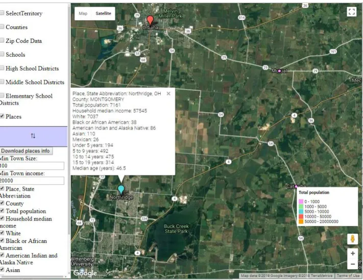
Figure 2 Towns are displayed on Google Maps with a legend about population in bottom right corner7

The web service was developed using the principle of multi-tenancy, where multiple users can access the service independently [26]. Users can select the relevant area, to view and download neccessary information in a CSV format. The solution makes possible to filter data geographically

7_{http://prep.swturf.eu/}

(20)

20 and intuitively for the users. In addition a filter was created to sort out towns by household median income and total population.

3.2.2 User interface

Figure 2 shows the interface of the web service. User interface was developed using HTML and CSS. User interface consists of two modules – layer selection panel and Google Maps8_{panel. The} functionality was written in JavaScript9_.

Using layer selection panel, user can select what kind of data it wants to render on the map. Layers should be the following:

• County layer • Town layer

• Zip Code area layer

• Census block group layer (not implemented yet) • School district boundaries

o High school districts

o Middle school district boundaries

o Elementary school district boundaries • Map of schools

8_{https://developers.google.com/maps/documentation/javascript/tutorial} 9_{https://www.javascript.com/}

(21)

21 Figure 3 Zip code tabulation areas colored according to household median income

3.2.3 Back end

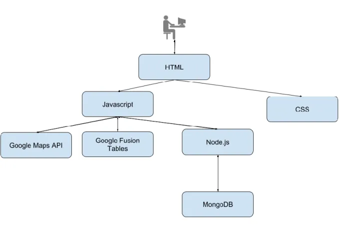
School district boundary files were hosted in MongoDB10_{. To interact with MongoDB, a} Node.js11_{server was set up. Other data layers we can see on the map are hosted on Google} Fusion Tables Platform.

10_{https://www.mongodb.com} 11_{https://nodejs.org/}

(22)

22 Boundary files are of considerable size (2.8 GB), which makes it not possible to store in Google Fusion Tables. Thus, the data was purified using Quantum GIS12_{and converted to GEOJSON}13 format. We ended up storing the data in MongoDB. We found after deployment that QGIS, makes it possible to simplify geometries, which would reduce the file size and make rendering school district boundaries faster [27].

Figure 4 Web service architecture

12_{https://qgis.org}

(23)

23

4 Methodology

4.1 Data preprocessing

4.1.1 GISJOIN and GEOID crosswalk

GISJOIN identifiers are used in NHGIS data tables. GEOID identifiers correspond to American FactFinder, TIGER/Line etc. These codes include all the information of every geographic census level starting from state identifier which are the first 2 or 3 digits of GEOID or GISJOIN code respectively. See Table 1 and Table 2 for the structure of both identifiers.

Component Notes

"G" prefix This prevents applications from automatically reading the identifier as a number and, in effect, dropping important leading zeros

State NHGIS code

3 digits (FIPS + "0"). NHGIS adds a zero to state FIPS codes to differentiate current states from historical territories.

County NHGIS code

4 digits (FIPS + "0"). NHGIS adds a zero to county FIPS codes to differentiate current counties from historical counties.

Census tract code

6 digits for 2000 and 2010 tracts. 1990 tract codes use either 4 or 6 digits.

Census block code

4 digits for 2000 and 2010 blocks. 1990 block codes use either 3 or 4 digits.

Table 1 GISJOIN identifier structure [28] Component Notes

State FIPS code 2 digits County FIPS

code

3 digits

Census tract code

6 digits. 1990 tract codes that were originally 4 digits (as in NHGIS files) are extended to 6 with an appended "00" (as in Census Relationship Files).

Census block code

4 digits for 2000 and 2010 blocks. 1990 block codes use either 3 or 4 digits.

Table 2 GEOID structure [28]

Data obtained from NHGIS had GISJOIN as identifiers and record of sales data had GEOID identifiers after geocoding. Thus, the identifiers had to be converted.

(24)

24

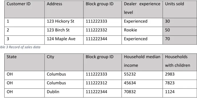
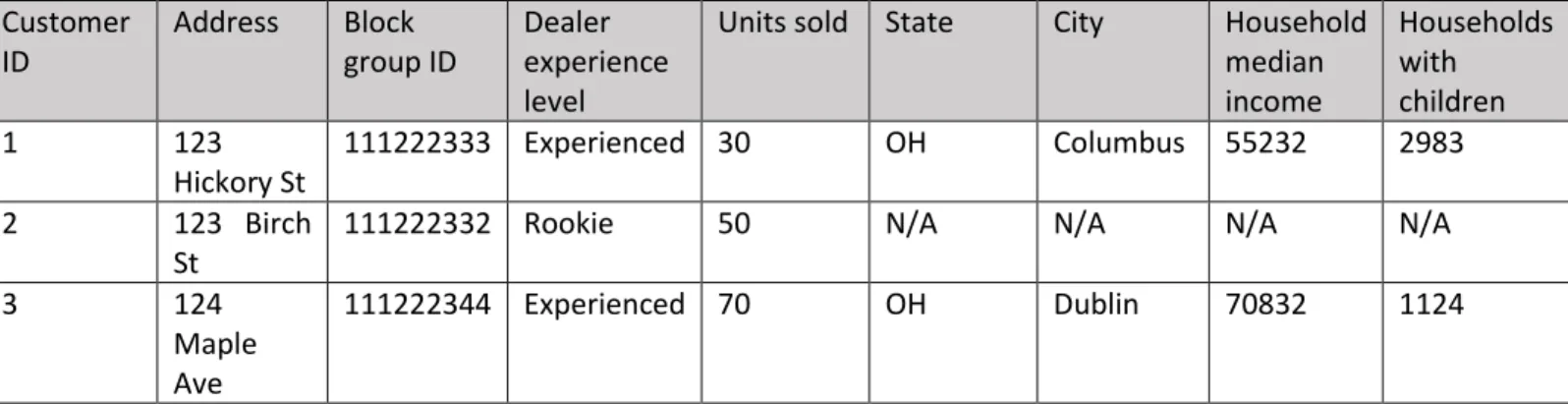
4.1.2 Matching data

Two tables Table 3 Table 4 could be matched by a key. In our case, the key could be block group ID. Left join creates a complete set of records from Table 3, with matching records from Table 4, where available. Left Join is illustrated by Figure 5.

Figure 5 Left join Venn diagram [29]

Customer ID Address Block group ID Dealer experience level

Units sold

1 123 Hickory St 111222333 Experienced 30

2 123 Birch St 111222332 Rookie 50

3 124 Maple Ave 111222344 Experienced 70

Table 3 Record of sales data

State City Block group ID Household median

income Households with children OH Columbus 111222333 55232 2983 OH Columbus 111222312 45634 7823 OH Dublin 111222344 70832 1124

(25)

25 Customer ID Address Block group ID Dealer experience level

Units sold State City Household median income Households with children 1 123 Hickory St 111222333 Experienced 30 OH Columbus 55232 2983 2 123 Birch St

111222332 Rookie 50 N/A N/A N/A N/A

3 124

Maple Ave

111222344 Experienced 70 OH Dublin 70832 1124

Table 5 Table 3 and Table 4 after left join has been performed.

A left join was performed joining record of sales data to demographic data, using block group id as the key. This is just a simplified example - actual datasets had more rows and columns. If there is no match N/A will be inserted [29].

4.1.3 Melting and casting data

Often data is collected and stored in a way optimized for ease and accuracy of collection. It doesn’t resemble the form necessary for statistical analysis. Therefore, reshaping data is a task that comes up often in real life data analysis. To be clear, data reshaping means rearranging the form of the data, but not the content.

Usually, we are used to think about data in terms of matrix or data frame, where observations are in the rows and variables are in columns. To understand reshaping, let’s divide the variables in two groups: identifier and measured variables.

Identifier variables identify the unit that measurement takes place on. In a database notation, id variables are referred to as a composite primary key.

Measured variables show what is measured on the unit.

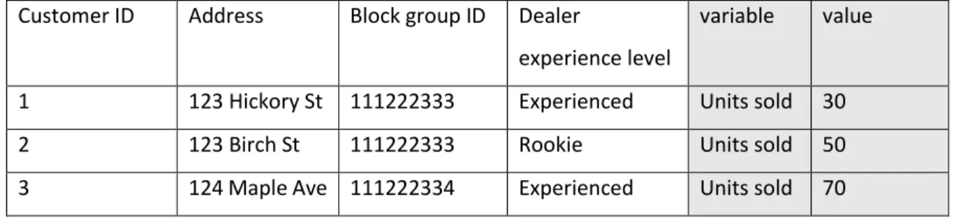
In our case we can rearrange Table 3 that has four id variables (Customer ID, Address, block group ID, Dealer experience level) to look like this:

(26)

26 Customer ID Address Block group ID Dealer

experience level

variable value

1 123 Hickory St 111222333 Experienced Units sold 30

2 123 Birch St 111222333 Rookie Units sold 50

3 124 Maple Ave 111222334 Experienced Units sold 70 Table 6 Molten data

This process is called melting data. The molten data has a new id variable ‘variable’, and a new column ‘value’. From now on, if we skip some of the original id variables in a new form, the combination of id variables will represent more than one observation. For example, we can summarize the data by Dealer experience level or on block group level. Aggregating data is also sometimes referred to as casting data. Table 7 shows aggregated data from Table 6 where ‘Units sold’ are summarized by ‘Dealer experience level’. Using this methodology, we melt and cast the data in numerous ways. We could also find out, what is the size of average sale by experience level etc [30].

Dealer

experience level

Units sold

Experienced 100

Rookie 50

(27)

27 4.2 Neural network

In many cases, relationship between input variables(covariates) and output variables (also known as response variables) are of big interest. For example, for a bank trying to predict which attributes would predict that it is safe to give out a loan to a person based on customers financial history. Neural network is an information processing paradigm, which is evolved during attempts to construct mathematical representation of information processing in biological systems. Neural networks have an ability to detect patterns and trends from data, where it would be too complex to be noticed by humans or other computer techniques [31]. Conventionally an algorithmic approach is used to solve problems i.e. computer takes specific steps that are pre-coded. This limits computer problem solving capability to problems that we already know how to solve. Neural networks are able to learn how to do tasks based on initial training data. The downside is that because the network finds out how to solve the problem independently, its operations might be unpredictable [16].

4.2.1 Multi-layer perceptron

The multi-Layer perceptron in its essence, is a directed graph that is made up by vertices and directed edges. In the contexts of artificial neural networks vertices are called neurons and edges are called synapses. Neurons are organized in layers that are usually connected fully by synapses. The input layer is made up of all covariates as separate neurons. The output layer is made up of response variables. Layers between input and output layers are referred to as hidden layers, since these layers are not directly observable. Input layer as well as the hidden layers have a neuron that is constant to account for synapses that are not affected by any of the input variables. This neuron is also referred to as bias unit [32].

(28)

28 Figure 6 Neural network with two input neurons (A and B), one output neuron (Y) and one hidden layer consisting of three hidden neurons. Bias unit is shown on the top [32].

The weight (𝑤_𝑖) attached to each of the synapse indicates the effect of a corresponding neuron. Most simple multi-layer perceptron is made up of input layer consisting of n covariates and output layer with one output neuron. It calculates the following function:

Equation 1 Simple multi-layer perceptron .

In this function, 𝑤₀ marks the intercept, vector 𝑾 = (𝑤₁, … , 𝑤_𝑛) is consisting of all weights without the bias unit.𝑿 = (𝑥₁, … , 𝑥_𝑛) is the vector representing all covariates.

For increasing modeling flexibility, we can include hidden layers. MLP with a hidden layer made up of 𝐽 hidden neurons. It calculates the following function:

(29)

29 Equation 2 MLP with hidden layer

where 𝑤₀ denotes the intercept of the output neuron. 𝑤_0𝑗 marks the intercept of 𝑗th hidden neuron. Also, 𝑤_𝑗 denotes weight corresponding to the synapse starting at the 𝑗th hidden neuron and going to the output neuron.

All hidden neurons and output neurons calculate an output 𝑓(𝑔(𝑧₀, 𝑧₁, … , 𝑧_𝑘)) = 𝑓(𝑔(𝒛)) from the output of all preceding neurons 𝑧0, 𝑧1, … , 𝑧𝑘, where 𝑔 is the integration function and 𝑓 the activation function. Integration function is usually 𝑔(𝒛) = 𝑤₀𝑧₀+ ∑_𝑖=1𝑘 𝑤_𝑖𝑧_𝑖 = 𝑤₀+ 𝒘𝑻𝒛. The activation function 𝑓 is often a bounded nonlinear and nondecreasing function e.g. logistic function (𝑓(𝑢) = 1

1+𝑒−𝑢) [32].

4.2.2 Supervised learning

Neural network fits to the data, using learning algorithms. This is called the training process. Given output is compared to the predicted output and the parameters are adjusted according to the comparison. Neural network parameters are its weights 𝒘. Weights are usually initialized with random values. The training process consist of following steps:

1. Neural network calculates an output 𝒐(𝒙)for given inputs 𝒙(also referred to as training set) and current weights. If the predicted output 𝒐 differs from the observed output 𝒚, then the training process continues.

2. Error function 𝐸 e.g. sum of squared errors (Equation 3) measures the difference between the predicted and observed output.

(30)

30 Equation 3 Sum of squared errors

In Equation 3 𝑙 = 1, … , 𝐿 indexes given input-output pairs, and ℎ = 1, … , 𝐻 the output nodes. 3. Weights are adjusted according to the learning algorithm.

Training process is being stopped when a pre-specified criterion is fulfilled. Usually, if all partial derivatives of the error function with respect to the weights _{(𝛿𝐸 𝛿𝑤}⁄ ) are smaller than predefined threshold. Backpropagation is the most commonly used learning algorithm [32].

4.2.3 Resilient backpropagation

The resilient backpropagation algorithm is very similar to the traditional backpropagation algorithm. Traditional backpropagation algorithm modifies weights of a neural network to find a local minimum of the error function. The gradient of the error function_{(𝑑𝐸 𝑑𝒘}⁄ ) is calculated with respect to the weights in order to find a root. Weights are modified in the opposite direction of the partial derivatives until a local minimum is reached. The idea for single variable error function is illustrated in Figure 7.

(31)

31 Figure 7 Basic concept for backpropagation algorithm illustrated for single variable error function [32]

The main difference between backpropagation and resilient backpropagation is the dynamic learning rate 𝜂_𝑘 in Equation 4. To speed up convergence in shallow areas (refer to Figure 7), the learning rate Re is increased until the corresponding derivative changes its sign. If the partial derivative is changes its sign, learning rate will be decreased since a changing sign means that the minimum was missed due to too large learning rate [33].

Equation 4 Resilient backpropagation weights adjustment

Last iteration will be undone by using weight backtracking and a smaller value will be added to the weight in the next step. Pseudocode is given by ref Riedmiller:

(32)

32 Pseudocode 1Resillient backpropagation [33]

4.2.4 Feature scaling

Some machine learning algorithms will not work well without normalization. Mostly, classifiers calculate distance between two points by the Euclidian distance. When some of the features have a wide range of values, the distance will be affected in big part by these features. Scaling is necessary, so that each feature would contribute proportionally to the final distance. Feature scaling makes gradient descent algorithm converge faster than without scaling.

The simplest way to scale is the so-called “Min-Max Scaling”. Using this method each feature is scaled to a fixed range [0,1]. This is done using the equation:

𝑋_{𝑛𝑜𝑟𝑚} = 𝑋−𝑋𝑚𝑖𝑛 𝑋𝑚𝑎𝑥−𝑋𝑚𝑖𝑛,

Where 𝑋_𝑚𝑖𝑛 is the minimum value of the feature and 𝑋_𝑚𝑎𝑥 is the maximum value of the feature.

(33)

33

5 Results and discussion

Using the methods discussed in Chapter 4, record of sales data was merged with demographic indicators and then aggregated to produce results discussed in current chapter.

5.1 Data analysis results

5.1.1 Sales results against dealer experience level

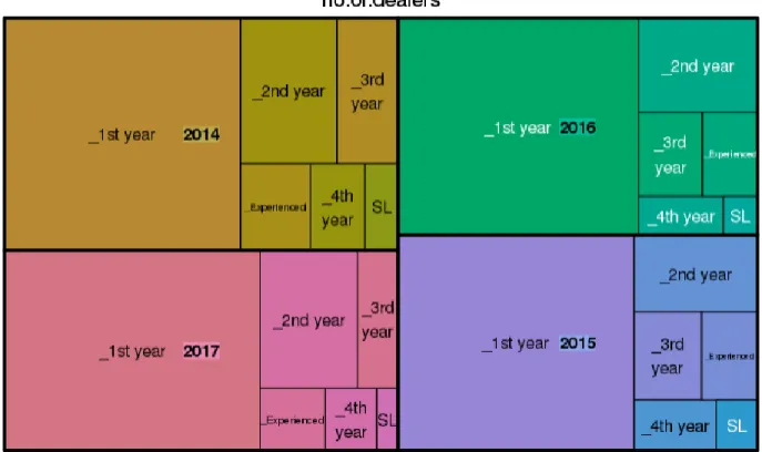
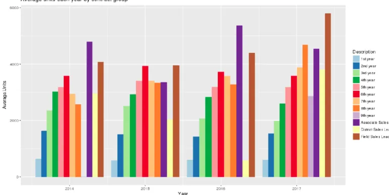
Figure 8 shows proportions of how many dealers company had by contract group last 4 years. The biggest group is the first-year dealers. The smallest group is the Sales Leaders. Figure 9 shows proportions of total revenue generated by contract group. Still, the first-year dealers are amounting to the biggest chunk of revenue, but their part is not proportional to the number of dealers in that group. This shows that experienced dealers are contributing more to the overall production than inexperienced dealers. This is illustrated more clearly in Figure 10 and Figure 11. As seen from Figure 10, dealer production tends to increase as dealer gains experience. This makes sense, because experienced dealers get more training. During training they learn and practice more sales techniques. Furthermore, as dealers gain more experience, the size of average sale goes up as well. This is illustrated by Figure 11. Figure 12 Shows average weekly production by contract groups. Error! Reference source not found. shows weekly sales by dealers i ndividually in 2017. We can see that there is a high concentration of dealers selling less than 250 units a week.

(34)

34 Figure 8 Number of dealers by contract group

(35)

35 Figure 10: Average units by year sold by contract group

(36)

36 Figure 12 Average weekly sales by contract group

(37)

37 Figure 13 Weekly production of individual dealers in 2017

5.1.2 Sales over time company wide.

(38)

38 Surprisingly, there is a strong pattern in company wide sales. Sales peak mid-July. Looking weekly patterns, then sales are higher on Saturdays (spikes on Figure 14) and sales are the lowest on Sundays (drops on Figure 14), because very few dealers go to sell on Sundays.

5.1.3 Sales against demographic data

5.1.3.1 Sales against income data

Figure 15 shows dealers individual weekly sales against household median income in the zip code area. The individual production is the highest in areas with household median income in between 45 000$ and 75 000$ a year.

Figure 15 Sales against household median income

5.1.3.2 Sales against family and population density

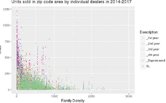
Figure 16 shows individual sales against family density in a zip code area. Counterintuitively, sales tend to be higher in areas with lower amount of families per square mile. The same occurs when looking at individual sales against population density in Figure 18,This could be due to the fact,

(39)

39 that first year dealers work mostly in suburban areas, which are accessible by bike. Managers work areas outside of cities, which could be reached by car. In Figure 17 we can see that sales tend to be higher if the percentage of families with children under 18 at home is close to 60 %. We can observe similar pattern also in Figure 15, where median household income is about 160000$ a year. This area could be classified as outlier, because it is very rarely occurring. Rest of the areas submit to normal distribution.

(40)

40 Figure 17 Sales against % of families having kids

(41)

41

5.1.4 Sales against sales in previous years in area

Figure 19 shows individual dealers performance against units sold in area previous years. We can see again, that sales tend to be higher in areas where less has been sold previous years. Yet, it doesn’t mean that one could not do well in an area where somebody has sold well just last year. This could be also because managers try to place salesforce to areas, that were not covered last year.

Figure 19 Weekly units of individual dealers plotted against units per households with children

5.1.4.1 Sales against dealers previous performance

Figure 20 - Figure 22 display clustering of production by dealer experience level. We can observe in Figure 20 that first-year dealers rarely sell more than 2000 units, many of the 2nd and 3rd_{year dealers sell anywhere between 2000 and 3000 units. Students selling their 4}th_year and up, are expected to sell 3000 to 6000 units. Leading the production, are the Sales Leaders

(42)

42 that most of the times reach more than 5000 units. From Figure 21 we can see that there is no telling if dealers next week production will be better than production last week, but there is a strong correlation with previous weeks production. This means that if a dealer is producing on a certain level one week, he or she is likely to continue with similar production. Comparing

current seasons production with last year production (Figure 22), we can see that majority of the times the observations fall above the black line. These data points indicate seasons where students have increased their production compared to previous year. We can still observe the clustering as in Figure 20.

(43)

43 Figure 21Weekly units against production last week

(44)

44 Figure 22 Dealers production this season against last years production

5.2 Data mining and predictions

5.2.1 Neural network structure

To train neural networks, data was normalized. Neural network had 3 hidden layers. Number of perceptrons for each layer was determined by the number of input variables 𝑛 with the following formula:

𝑁𝑁_{𝑠𝑡𝑟𝑢𝑐𝑡} = (1.5𝑛; 𝑛; 0.5𝑛)

Thus, having data with 8 input variables would yield a neural network with 𝑁𝑁_{𝑠𝑡𝑟𝑢𝑐𝑡} = (12; 8; 4).

Data from 2017 was used for testing and the rest was left for training the network. When performance from previous year was used as a feature, data from 2014 was discarded, because we didn’t have data from 2013.

(45)

45 Figure 25 shows neural network performance with the X- axis representing actual results (test.r) in the test set and Y-axis representing neural network predictions (pr.nn_). The line in the middle would show ideal performance where all the predictions would be correct. To evaluate performance, mean square error was used. The reader can interpret Figures Figure 24Figure 25Figure 26Figure 27 in the same manner.

5.2.2 Evaluating neural network performance

When dealing with classification problems, machine learning algorithms are evaluated mostly by their accuracy.

𝐴𝑐𝑐𝑢𝑟𝑎𝑐𝑦 = 𝑡𝑟𝑢𝑒 𝑝𝑜𝑠𝑖𝑡𝑖𝑣𝑒𝑠 + 𝑡𝑟𝑢𝑒 𝑛𝑒𝑔𝑎𝑡𝑖𝑣𝑒𝑠

𝑡𝑟𝑢𝑒 𝑝𝑜𝑠𝑖𝑡𝑖𝑣𝑒𝑠 + 𝑓𝑎𝑙𝑠𝑒 𝑝𝑜𝑠𝑖𝑡𝑖𝑣𝑒𝑠 + 𝑡𝑟𝑢𝑒 𝑛𝑒𝑔𝑎𝑡𝑖𝑣𝑒𝑠 + 𝑓𝑎𝑙𝑠𝑒 𝑛𝑒𝑔𝑎𝑡𝑖𝑣𝑒𝑠

Evaluating neural network with linear output is different. Mean square error is used to measure the differences between predicted values and observed values.

𝑀𝑆𝐸 =1

𝑛∑|𝑦𝑗− 𝑦𝑗

′_| 𝑛

𝑗=1

(46)

46

5.2.3 Predicting sales by contract group over time

Figure 23 Prediction of average daily sales by contract group

Figure 14 shows a clear pattern in sales company wide. Sales seem to be affected by the week number and day of the week. We could argue that people have higher motivation at the beginning of the work week after a day off. Also, on Sundays, there are group meetings, which supposedly boost motivation in sales force. The peaks on Saturdays could be also explained, because people are at home and on Saturdays most of companies dealers are working callbacks, this means that sales people are wasting less time on mapping out the area. It might be also explained by having higher motivation, because the work week is ending with Saturday. In Figure 10 we can see, that production is also dependent on the level of experience of a dealer. Therefore, a separate neural network was trained for each experience level. Figure 23 shows neural network predictions (red line) against the actual averages (green line) in 2017.

Figure 23 shows neural network performance while trying to predict average units by contract group each day.

(47)

47

Contract group Mean square error

1st_year _4.56 2nd_year _6.19 3rd_year _27.8 4th_year _122.67 Experienced dealers 46.07 Sales Leader 237.01

5.2.4 Predictions using dealer characteristics and demographic data

We tried to feed different features to our neural network. Surprisingly, it turned out that demographic features don’t predict sales results too well. Mixing demographic features to dealer experience and past performance characteristics worsens the results of the prediction algorithm.

Input features Mean square error Performance

figure Household median income, Family density,

Units per households with children last year

29354.78 Figure 24

Description, Dealer ID, Week, Dealer Units Last Week, Dealer Units Last Year

3776.82 Figure 25

Description, Dealer ID, Week, Dealer Units Last Week, Dealer Units Last Year, Household media n income, Family density, Units per households with children last year

6400.95 Figure 26

Description, Dealer ID, Week Dealer Units Last Week, Units per households with children last year

(48)

48 Figure 24 Household median income, Family density, Units per households with children last year

(49)

49 Figure 26 Description, Dealer ID, Week, Dealer Units Last Week, Dealer Units Last Year,

(50)

50 Figure 27 Description, Dealer ID, Week Dealer Units Last Week, Units per households with children last year

5.3 Conclusion

We see that there are patterns in the data. We saw also, that success in sales was not affected as much by the area as it was affected by characteristics of a specific dealer and week in the year. Thus, we can say that selling is a skill that one acquires over the years and has not much to do with the area someone is placed in. Drawing conclusions from Figure 23 the author suggests the sales management to place a motivational event on Wednesday, since this is the lowest day in production.

In this thesis data is not presented against block group indicators. The aim was to find out, what would increase weekly production. The issue we ran into was that dealers might work in many different block group areas, which makes data too granular to look on a block group level to reveal any patterns in dealer’s weekly performance. On the other hand, geocoding the record of sales data will be beneficial in future visualizations.

(51)

51

6 Conclusion and future perspectives

6.1 Conclusion

This thesis had three main objectives:

1. Visualize demographic and sales data on a map

2. Analyze relationship between sales performance against demographic indicators and dealer characteristics

3. Develop predictive models based on analysis.

To sum up, we can state that the thesis has been a success. The web service for pulling and visualizing data has been accepted and in constant use by the sales managers and organizational leaders in the company. In data analysis we were able to find some interesting relationships between sales performance, demographic indicators and dealer characteristics. Building predictive models revealed that demographic indicators don’t affect sales performance as much as dealer characteristics. It might be argued that experienced dealers are able to select better areas for themselves, but we are not able to conclude this within the scope of this thesis.

6.2 Future perspectives

6.2.1 Future perspectives for the web service

Hopefully, the web service developed within this thesis will serve as a prototype for future solutions and will be a valuable tool for planning workable territories for company’s management. There are many improvements that could be implemented in the future versions. There have been requests that demographic information could be merged also into the county layer and school district layers. To get more granular insights, data should be visualized also on block group level. From company’s databases potential host families and requirements to get solicitor permits could be displayed on the map for more intuitive planning of summer logistics.

(52)

52 Would be nice to have downloadable data already aggregated by the system. To enhance usability, the web service should be integrated with company’s internal systems. This would allow user to save its territory selection and continue from where he or she left off, when reloading the page. Currently, user must make geographical selection again every time system is refreshed. Also, we could have the system to aggregate data within its back end. This would eliminate the need for managing many custom spreadsheets by the management. Having these enhancements it could be possible to implement a territory planning algorithm based on the criteria and data available in the system.

6.2.2 Future perspectives for data analysis and predictions

With writing this thesis, the author developed a new skill set and framework to aggregate and visualize data quickly. This helps answering future queries and verifying or refuting future hypothesis stated by the management. To improve the predictive models, more research could be done by trying to predict with various combinations of attributes to minimize prediction error. There might be other attributes predicting sales performance that we haven’t investigated. For example, dealers work statistics could be also matched with dealers other characteristics and demographic data to produce even better results.

(53)

53

References

[1] A. Mislove, L. Sune, Y.-Y. Ahn, J.-P. Onnela and J. N. Rosenquist, "Understanding the Demographics of Twitter Users.," ICWSM, vol. 11, no. 5, p. 25, 2011.

[2] E. F. M. A. H. C. J. P. Ian H. Witten, I. H. Witten, F. Eibe, M. Hall and C. J. Pal, Data Mining: Practical Machine Learning Tools and Techniques.

[3] U. Fayyad, A. Wierse and G. Grinstein, Information Visualization in Data Mining and Knowledge Discovery, Morgan Kaufmann, 2002.

[4] C. Jones, Geographical Information Systems and Computer Cartography, Taylor \& Francis, 2014. [5] D. Li and S. Wang, Spatial Data Mining: Theory and Application, Springer Berlin Heidelberg, 2016. [6] Tamsin, P. Warr and D. Bartram, "Personality and Sales Performance: Situational Variation and

Interactions between Traits},," International Journal of Selection and Assessment, vol. 13, no. 1, pp. 87-91.

[7] G. Linoff and M. Berry, Data Mining Techniques: For Marketing, Sales, and Customer Relationship Management, Wiley, 2011.

[8] K. Au and N. Chan, "Quick response for Hong Kong clothing suppliers : a total system approach," in Proceedings of the Annual Conference of the Production and Operations Management Society,, San Francisco, USA, 2002.

[9] R. Kuo, "A sales forecasting system based on fuzzy neural network with initial weights generated by genetic algorithm," European Journal of Operational Research, vol. 129, no. 3, pp. 496--517, 2001.

[10] M. Giering, "Retail sales prediction and item recommendations using customer demographics at store level," ACM SIGKDD Explorations Newsletter, vol. 10, no. 2, pp. 84-89, 2008.

[11] E. W. Frees and T. W. Miller, "{Sales forecasting using longitudinal data models," International Journal of Forecasting, vol. 20, no. 1, pp. 99-114, 2004.

[12] G. a. B. M. Linoff, "Data Mining to improve direct marketing campaigns," in Data Mining

Techniques: For Marketing, Sales, and Customer Relationship Management, Wiley, 2011, pp. 41-46.

[13] Y.-W. Wang and P.-C. Chang, "Fuzzy Delphi and back-propagation model for sales forecasting in PCB industry," Expert systems with applications, vol. 30, no. 4, pp. 715-726, 2006.

[14] C. Frank, A. Garg, L. Sztandera and A. Raheja, "Forecasting women's apparel sales using

mathematical modeling," International Journal of Clothing Science and Technology, vol. 15, no. 2, pp. 107-125, 2003.

(54)

54 [15] S. Beheshti-Kashi, R. Karimi, T. Hamid, K.-D. Lütjen and M. Teucke, "A survey on retail sales

forecasting and prediction in fashion markets," in Systems Science & Control Engineering: An Open Access Journal, 2015, pp. 154-161.

[16] C. Bishop, Neural networks for pattern recognition, Oxford university press, 1995. [17] W. Aref and H. Samet, "Extending a DBMS with spatial operations," in Advances in Spatial

Databases.

[18] US Census Bureau, [Online]. Available:

https://www2.census.gov/geo/pdfs/reference/geodiagram.pdf. [Accessed 2018].

[19] National Center for Education Statistics, "School attendance boundaryu survey," [Online]. Available: https://nces.ed.gov/programs/sabs/. [Accessed 2018].

[20] National Center for Education Statistics, "Search for Public Schools," [Online]. Available: https://nces.ed.gov/ccd/schoolsearch/. [Accessed 2018].

[21] Integrated Public Use Microdata Series, "IPUMS org," [Online]. Available: https://www.ipums.org/whatIsIPUMS.shtml. [Accessed 2018].

[22] Integrated Public Use Microdata Series, "What is NHGIS?," [Online]. Available: https://www.nhgis.org/user-resources/project-description.

[23] US Census Bureau, "American Community Survey," [Online]. Available: https://www.census.gov/programs-surveys/acs/. [Accessed 2018]. [24] US Census Bureau, "U.S. Census TIGER/Line," [Online]. Available:

http://www.gdal.org/drv_tiger.html. [Accessed 2018].

[25] F. C. Commission, "Census Block Conversions API," [Online]. Available: https://www.fcc.gov/census-block-conversions-api. [Accessed 2018]. [26] M. Rouse, "DEFINITION multi-tenancy," [Online]. Available:

https://whatis.techtarget.com/definition/multi-tenancy. [Accessed 2018].

[27] J. A. C.-L. a. M. B.-G. a. A. F. a. M. R. Luaces, J. Luaces, L. Cotelo, M. Barcon-Goas and A. Farina, "Combining Geometry Simplification and Coordinate Approximation Techniques for Better Lossy Compression of GIS Data," in Data Compression Conference, 2013.

[28] IPUMS, "Geographic crosswalks," [Online]. Available: https://www.nhgis.org/user-resources/geographic-crosswalks. [Accessed 2018].

[29] Stitch, "SQL join," [Online]. Available: http://www.sql-join.com/sql-join-types/. [Accessed 2018]. [30] H. A. Wickham, Practical tools for exploring data and models, Iowa State University, 2008.

(55)

55 [31] A. Galushkin, Neural Network Theory. Secaucus, NJ, USA: Springer-Verlag New York, Inc, 2007. [32] G. Frauke and S. Fritsch, "neuralnet: Training of neural networks," The R journal, pp. 30--38, 2010. [33] M. Riedmiller and H. Braun, "A direct adaptive method for faster backpropagation learning: The

RPROP algorithm," in Neural Networks, 1993., IEEE International Conference on, 1993.

[34] S. Aksoy, H. Aksoy and R. M. , "Feature normalization and likelihood-based similarity measures for image retrieval," Pattern recognition letters, pp. 563-582, 2001.

[35] D. M. W. Powers, "Evaluation: From Precision, Recall and F-Measure to ROC, Informedness, Markedness & Correlation," Journal of Machine Learning Technologies, vol. 2, no. 1, pp. 37-63, 2011.

[36] W. Leigh, R. Purvis and J. Ragusa, "Forecasting the NYSE composite index with technical analysis, pattern recognizer, neural network, and genetic algorithm: a case study in romantic decision support," Decision support systems, vol. 32, no. 4, pp. 361-377, 2002.

(56)

56

Licence

Non-exclusive licence to reproduce thesis and make thesis public

I, Taavi Ilmjärv,

1. herewith grant the University of Tartu a free permit (non-exclusive licence) to:

1.1. reproduce, for the purpose of preservation and making available to the public, including for addition to the DSpace digital archives until expiry of the term of validity of the copyright, and

1.2. make available to the public via the web environment of the University of Tartu, including via the DSpace digital archives until expiry of the term of validity of the copyright,

„Sales and demographic data visualization, analysis and forecasting“ ,supervised by Amnir Hadachi,

2. I am aware of the fact that the author retains these rights.

3. I certify that granting the non-exclusive licence does not infringe the intellectual property rights or rights arising from the Personal Data Protection Act.