Pricing default swaps: empirical evidence

Pricing Default Swaps: Empirical Evidence

Patrick Houweling

Erasmus University Rotterdam

Rabobank International

Ton Vorst

Erasmus University Rotterdam

ABN Amro

November 14, 2003

Abstract

In this paper we compare market prices of credit default swaps with model prices. We show that a simple reduced form model outperforms directly com-paring bonds’ credit spreads to default swap premiums. We find that the model yields unbiased premium estimates for default swaps on investment grade issuers, but only if we use swap or repo rates as proxy for default-free interest rates. This indicates that the government curve is no longer seen as the reference default-free curve. We also show that the model is relatively insensitive to the value of the assumed recovery rate.

JEL codes: C13, G12, G13

Keywords:

credit default swaps, credit risk, default risk, recovery rates, reduced form models

Forthcoming in theJournal of International Money and Finance

1_{Corresponding author. Current contact details: Robeco Asset Management, P.O Box 973,} 3000 AZ Rotterdam, The Netherlands; tel: +31-10-244.3538; fax: +31-10-244.2164; e-mail:

p.houweling@robeco.nl

1

Introduction

During the last decade, credit derivatives have become important instruments to lay off or take on credit risk. The credit derivatives market has grown exponentially. Until today only very limited empirical research has been devoted to these new instruments, although several reduced form models have been developed to price them. Most empirical papers on credit risk modelling have focussed on defaultable bonds. In this paper, we estimate reduced form models and compare model-implied credit default swap premiums to market data. We show that a reduced form model gives more accurate estimates of default swap premiums than bonds’ yield spreads. Moreover, we shed light on the choice of the default-free term structure of interest rates. We find that swap and repo curves significantly outperform the government curve as proxy for default-free interest rates for investment grade issuers, but that their performance is similar for speculative grade issuers. As such, this is one of the first studies to empirically confirm that financial markets no longer see Treasury bonds as the default-free benchmark.

A default swap protects its buyer from losses caused by the occurrence of a default event to a debt issuer. In exchange for this default protection, the buyer pays a periodic premium to the protection seller. The no-arbitrage value of the default swap premium can be derived by applying a reduced form credit risk model. In these models, prices of default-sensitive instruments are determined by the risk-neutral default probability and the recovered amount at default. Default is often represented by a random stopping time with a stochastic or deterministic hazard rate, while the recovery rate is often assumed to be constant. We have a large data set of market quotes on credit default swaps at our disposal. This allows us to conduct empirical testing of reduced form models, which

the literature has lacked so far. To the best of our knowledge, the only other study that analyses credit default swap data is Aunon-Nerin et al. (2002). Their primary analyses are regressions of default swap premiums on proxies for credit risk, whereas we estimate and apply a reduced form credit risk model. Aunon-Nerin et al. (2002) also implement the Das and Sundaram (2000) tree model, but on just 75 observations. Moreover, they used spread curves per rating-sector combination, while we apply our models per issuer.

As a first indication, the default swap premium is often estimated by the yield spread of a bond with a similar maturity issued by the same borrower. We show analytically that this relationship only holds approximately. Moreover, we show empirically that the ap-proximation results in fairly large deviations between calculated and market default swap premiums. By deriving the risk-neutral pricing formula for a defaultable coupon-bearing bond, we can explicitly express its dependence on risk-neutral processes for default-free interest rates, hazard rates and and the recovery rate. Since we focus on the estima-tion and applicaestima-tion of credit risk models, we use a priori estimated default-free term structures. The choice for default-free interest rates has received little attention in the literature. Virtually all empirical papers on credit risk modelling used zero-coupon rates extracted from government bonds. However, since 1998, financial markets have moved away from estimating default-free interest rates from government securities, and started using swap and repo contracts instead. We find that using the government curve results in statistically significant overestimation of credit risk for investment grade issuers, that using swap curves result in a small but significant bias, and that using repo curves yields unbiased estimates. For speculative grade issuers, the choice for the default-free curve is less important, as the performance differences between the three curves are smaller.

to extract both the hazard rate and the recovery rate from prices of bonds of a single seniority class, we fix the recovery rate to identify the model. We show that not only bond spreads, but also default swap premiums are relatively insensitive to changes in the recovery rate as long as the hazard function is scaled accordingly. Therefore, there is no need to determine the recovery rate very accurately, as long as it takes a reasonable value. We model the hazard function as a constant, linear or quadratic function of time to maturity. The parameters of the hazard function are estimated using non-linear least squares from market prices of bonds of a single issuer. The estimated credit model is subsequently applied to the pricing of credit default swaps written on the same issuer. We observe that both the in-sample fit to bonds and the ‘out-of-sample’ fit to default swaps declines with an issuer’s credit quality. We also find that using the various hazard rate functions yield more accurate estimates of default swap premiums than directly using the yield spread of a similar bond. An analysis of the deviations between calculated and market premiums reveals that the deviations for all models are related to the maturity of the default swap and the rating of the underlying issuer.

The remainder of this paper is structured as follows. Section 2 discusses the charac-teristics of credit default swaps. The literature on reduced form credit risk modelling is reviewed in Section 3. In Section 4, we derive reduced form valuation models for bonds and default swaps, and present our estimation framework. The construction of our data set is outlined in Section 5. In Section 6 we present the results of applying the direct com-parison methods and the reduced form models. Finally, Section 7 concludes the paper.

2

Default Swaps

Default swaps are the most popular type of credit derivatives: according to the latest Credit Derivatives Survey by the British Bankers’ Association (BBA, 2002) they account for 45% of the global credit derivatives market and according to the most recent Credit Derivatives Survey by Risk Magazine (Patel, 2003) for even 73%. A default swap is a contract that protects the holder of an underlying obligation from the losses caused by the occurrence of a credit event to the obligation’s issuer, referred to as the reference entity. Credit events that trigger a default swap can include one or more of the follow-ing: bankruptcy, failure to make a principal or interest payment, obligation acceleration, obligation default, repudiation/moratorium (for sovereign borrowers) and restructuring; these events are jointly referred to as default. A default swap only pays out if the ref-erence entity defaults; reductions in value unaccompanied by default do not compensate the buyer in any way. Also, the default event must be verifiable by publicly available information or an independent auditor. The protection buyer either pays an up-front amount or makes periodic payments to the protection seller, typically a percentage of the notional amount. In the latter case, the percentage that gives the contract zero value at initiation is called the spread, premium or fixed rate. If default occurs, the default swap can be settled in one of two ways. With acash settlement, the buyer keeps the underlying asset(s), but is compensated by the seller for the loss incurred by the credit event. In a physical settlement procedure, the buyer delivers the reference obligation(s) to the seller, and in return, he receives the full notional amount. Either way, the value of the buyer’s portfolio is restored to the initial notional amount.

pe-riodic payments, and default occurs, the buyer is typically required to pay the part of the premium payment that has accrued since the last payment date; this is called the accrual payment. The credit event may apply to a single reference obligation, but more commonly the event refers to any one of a much broader class of debt securities, includ-ing bonds and loans. Similarly, the delivery of obligations in case of physical settlement can be restricted to a specific instrument, though usually the buyer may choose from a list of qualifying obligations, irrespective of currency and maturity as long as they rank pari passu with (have the same seniority as) the reference obligation. This latter feature is commonly referred to as the delivery option. Theoretically, all deliverable obligations should have the same price at default and the delivery option would be worthless. How-ever, in some credit events, e.g. a restructuring, not all obligations become immediately due and payable, so that after such an event bonds with different characteristics will trade at different prices. This is favorable to the buyer, since he can deliver the cheapest bonds to the seller. Counterparties can limit the value of the delivery option by restricting the range of deliverable obligations, e.g. to non-contingent, interest-paying bonds.

Counterparty risk is generally not taken into account in determining deal prices; if a party is unwilling to take on credit risk to its counterparty, it either decides to cancel the trade or to alleviate the exposure, e.g. by demanding that a collateral is provided or that the premium is paid up-front instead of periodically (Culp and Neves (1998) and O’Kane and McAdie (2001)).

An important application of default swaps is shorting credit risk. The lack of a market for repurchase agreements (repos) for most corporates makes shorting bonds unfeasible. So, credit derivatives are the only viable way to short corporate credit risk. Even if a bond can be shorted on repo, investors can only do so for relative short periods of time

(one day to one year), exposing them to changes in the repo rate. On the other hand, default swaps allow investors to go short credit risk at a known cost for long time spans: default swaps with maturities of up to 10 years can be easily contracted, but liquidity rapidly decreases for even longer terms.

3

Literature

In the literature, there are two approaches to price bonds and credit derivatives. In the class of structural models, due to Black and Scholes (1973) and Merton (1974), a firm defaults when the value of the firm’s assets drops below a certain threshold. The parameters of such models are hard to estimate, because the assets’ market value and volatility are difficult to observe. In reduced form models, developed by Litterman and Iben (1991), Jarrow and Turnbull (1995) and Jarrow et al. (1997), the direct reference to the firm’s asset value process is abandoned. Instead, credit risk is determined by the occurrence of default and the recovered amount at default. Default is often represented by a random stopping time with a stochastic or deterministic arrival intensity (hazard rate), while the recovery rate is usually assumed to be constant. In a somewhat different approach, due to Longstaff and Schwartz (1995), Duffie and Singleton (1999) and Das and Sundaram (2000), there is no need to separately model the hazard and recovery components of credit risk, but it suffices to model the spread process. In this paper, we use a reduced form model in the spirit of Jarrow and Turnbull (1995).

The empirical literature on reduced form models has focused on estimating the param-eters of one of three processes: the hazard process, the spread process or the risky short rate process. The first approach seems to be most popular. Cumby and Evans (1997)

considered both cross-sectional estimation of a constant hazard rate model and time-series estimation of several stochastic specifications. Madan and Unal (1998) estimated recovery and hazard processes in a two-step procedure using Maximum Likelihood (ML) and Gen-eralized Methods of Methods (GMM). Duffee (1998), Keswani (2000) and Driessen (2001) applied ML with Kalman filtering to obtain parameter estimates of Cox-Ingersoll-Ross (CIR) processes from time-series data. Bakshi, Madan and Zhang (2001), Fr¨uhwirth and S¨ogner (2001) and Janosi et al. (2002) used non-linear least squares to estimate the model parameters from cross-sectional data. Janosi et al. specified a stochastic hazard rate that depends on the default-free short rate and an equity market index; Bakshi et al. estimated a model with correlated interest rates, hazard rates and recovery rates; Fr¨uhwirth and S¨ogner used a constant hazard rate.

The second approach applies the Duffie and Singleton (1999) framework by directly estimating the spread process. Nielsen and Ronn (1998) estimated a log-normal spread model using non-linear least squares from cross-sectional data. Taur´en (1999) utilized GMM to estimate the spread dynamics as a Chan et al. (1992) process. D¨ulmann and Windfuhr (2000) and Geyer et al. (2001) implemented a ML procedure with Kalman filtering to obtain parameter estimates of Vasicek and/or CIR models for the instantaneous spread. Duffie et al. (2003) used an approximate Maximum Likelihood method to estimate a multi-factor model with Vasicek and CIR processes.

The third approach is to consider the sum of the default-free rate and the spread and estimate a model for the total risky rate. Duffie and Singleton (1997) utilized this approach to estimate the swap rate as a 2-factor CIR process using Maximum Likelihood. All discussed papers assessed the quality of the models on their ability to fit spreads or bond prices. Since credit derivatives allow credit risk to be traded separately from

other sources of risk, they provide a clean way of putting a price on credit risk. So, we may obtain better insights in the performance of credit risk models by applying them to the pricing of credit derivatives.

4

Methodology

In this section, we first discuss the valuation of bonds and credit default swaps in our reduced form credit risk model. Then, we elaborate on the specification and estimation of the model.

4.1

Valuing Bonds

Following Jarrow and Turnbull (1995), we assume a perfect and arbitrage-free capital market, in which default-free and defaultable zero-coupon bonds, a default-free money-market account and defaultable coupon bonds are traded. Uncertainty is represented by a filtered probability space (Ω,F,Q), where Ω denotes the state space, F is a σ-algebra of measurable events in Ω and Q is the actual probability measure. The information structure is represented by the filtration F(t). We take as given some non-negative, bounded and predictable default-free short-rate processr(t), which drives the default-free money-market account B(t). Let ˜Q denote the equivalent martingale measure that is associated with the numeraire B(t); see Harrison and Pliska (1981). That is, ˜Q is the risk-neutral measure. Letp(t, T) andv(t, T) denote the time-tvalues of adefault-free and a defaultable zero-coupon bond with maturity T and face value 1. Default occurs at a random timeτ, independent ofr(t) under ˜Q.1 _{Let ˜P(t, T) denote the risk-neutral survival}

1_{In our empirical application, we use readily available default-free term structures instead of specifying}

probability, i.e. ˜P(t, T) = ˜Et[1{τ >T}] with ˜Et[X] = EQ˜ [X|Ft] and 1{A} the indicator

function of event A. We assume the existence of a non-negative, bounded and predictable process λ(t), which represents thedefault intensity orhazard rate for τ under ˜Q. Then,

˜ P(t, T) = ˜Et · exp µ − Z _T t λ(s)ds ¶¸ = ˜Et[exp(−Λ(t, T))], (1)

where Λ(t, T) denotes theintegrated hazard function: Λ(t, T) =R_tT λ(s)ds.

Now, consider a defaultable coupon bond with coupon payment dates t= (t1, . . . , tn),

coupon payment c, maturity tn and notional 1. We assume that a constant2 recovery

fractionδof the notional (andnot of the remaining coupons too, see Jarrow and Turnbull (2000) and Sch¨onbucher (2000)) is paid at the random default time τ. To calculate the price v(t,t, c) of this bond, we apply the risk-neutral valuation principle to the coupon, notional and recovery cash flows (cf. Duffie and Singleton, 1997, Equation (26))

v(t,t, c) = n X i=1 p(t, ti)˜Et £ c1{τ >ti} ¤ +p(t, tn)˜Et £ 1{τ >tn} ¤ + ˜Et £ p(t, τ)δ1{τ≤tn} ¤ = n X i=1 p(t, ti)cP(˜ t, ti) +p(t, tn)˜P(t, tn) + Z _tn t p(t, s)δf(s)ds, (2)

where f(t) denotes the probability density function associated with the intensity process

λ(t). In our empirical application, we replace the integral in Equation (2) by a numerical approximation:3 _{we define a monthly grid of maturities s}

0, . . . , sm, where s0 = t and between default-free rates and the default time, so there is no use in allowing for a correlation parameter in our model.

2_{If we assume a stochastic recovery rate that is risk-neutrally independent from the default-free}

short-rate process and the default time, all formulas remain valid, except thatδ should be interpreted as the

expected recovery rate under the risk-neutral measure. Moreover, the results of Bakshi et al. (2001)

indicated that a model with a stochastic recovery rate performs equally well as a model with a constant recovery rate.

3_{This approximation is necessary, because we do not have an analytical expression forp(t,·), but use}

sm =tn and set Z _tn t p(t, s)δf(s)ds≈ m X i=1 p(t, si)δ ³ ˜ P(t, si−1)−P(˜ t, si) ´ .

4.2

Valuing Default Swaps

A default swap contract consists of a fixed leg and a floating leg. The former contains the payments by the buyer to the seller; it is called the fixed leg, because its payments are known at initiation of the contract. The floating leg comprises the potential payment by the seller to the buyer; at the start date, it is unknown how much the seller has to pay (if he has to pay at all).

Consider a default swap contract with payment dates T= (T1, . . . , TN), maturityTN,

premium percentage P and notional 1. Denoting the value of the fixed leg by ¯V(t,T, P) and the value of the floating leg by ˜V(t), the value of the default swap to the buyer equals

˜

V(t)−V¯(t,T, P). At initiation, the premium P is chosen in such a way that the value of the default swap is equal to zero. Since the value of the fixed leg is homogeneous of degree one in P, the premium percentage should be chosen as P = ˜V(t)/V¯(t,T,1).

We first determine the value of the fixed leg. At each payment date Ti, the buyer has

to pay α(Ti−1, Ti)P to the seller, where α(Ti−1, Ti) is the year fraction between Ti−1 and

Ti (T0 is equal tot). If the reference entity does not default during the life of the contract, the buyer makes all payments. However, if default occurs at time s≤TN, the buyer has

made only I(s) payments, where I(s) = max(i = 0, . . . , N : Ti < s) and the remaining

payment of α(TI(s), s)P at times.4 The value of the fixed leg at time t is thus equal to ¯ V(t,T, P) = N X i=1 p(t, Ti)˜Et £ α(Ti−1, Ti)P1{τ >Ti} ¤ + ˜Et £ p(t, τ)α(TI(τ), τ)P1{τ≤TN} ¤ = N X i=1 p(t, Ti)α(Ti−1, Ti)PP(˜ t, Ti) + Z _TN t p(t, s)α(TI(s), s)P f(s)ds. (3)

Next, we calculate the value of thefloating leg. If the contract specifiescash settlement, the buyer keeps the reference obligation at default and the seller pays the buyer the difference between the reference price and the final price. The reference price typically equals 100%. The final price is the market value of the reference obligation at the default date;5 _{under our recovery assumption, the final price is equal to δ, so that the value of} the floating leg under cash settlement equals

˜ V(t) = ˜Et £ p(t, τ)(1−δ)1{τ≤TN} ¤ = Z _TN t p(t, s)(1−δ)f(s)ds. (4)

If the contract specifiesphysical settlement, the buyer delivers deliverable obligations with a total notional of 1 to the seller and the seller pays 1 in return. Assuming one deliverable, the value of the floating leg is equal to Equation (4). However, a default swap contract generally has a delivery option (see Section 2), allowing the buyer to choose from a list of qualifying obligations. We refrain from valuing the delivery option, and use the value of the floating leg under cash settlement. To numerically approximate the integrals in Equations (3) and (4), we use the same method as for the defaultable coupon bond price.

4_{We assume that if the default time exactly coincides with a payment date Ti, the buyer does not}

make the regular payment, but makes an accrual payment, i.e. I(Ti) =i−1. Since the regular payment and the accrual payment are equal on a payment date, this assumption does not affect the value of the default swap.

5_{Commonly, the calculation agent has to poll one or more dealers for quotes on the reference}

Again, a monthly grid is chosen.

Our default swap pricing formula is very similar to other models encountered in the literature. The models by Aonuma and Nakagawa (1998), Brooks and Yan (1998), Scott (1998), Jarrow and Turnbull (1998) and Duffie (1999) are equal to our model, except that they only allow defaults on premium payment dates. Nakagawa (1999) and Hull and White (2000), like us, also allowed defaults to occur on other dates than payment dates. However, Nakagawa (1999) did not incorporate the accrual payment and Hull and White (2000) assumed that the protection buyer makes a continuous stream of premium payments, rather than a set of discrete payments.

4.3

Specification

Since we focus on credit risk models, we refrain from estimating a model for the default-free short-rate. Instead, we use a priori estimated curves to calculate the prices of default-free zero-coupon bonds. To completely specify the model, we have to (i) select the risk-neutral hazard model, (ii) pick a recovery rate and (iii) choose a proxy for the default-free term structure.

4.3.1 Hazard Process

In the literature discussed in Section 3, all studies that use time series estimation model the hazard rate stochastically, typically as a Vasicek or CIR process. Papers that use cross-sectional estimation consider either constant or stochastic hazard rates, where the stochastic process is chosen in such a way that the survival probability curve in Equa-tion (1) is known analytically. We follow an intermediate approach by using a deter-ministic function of time to maturity. This specification facilitates parameter estimation,

while still allowing for time-dependency. We model the integrated hazard function as a polynomial function of time to maturity

Λ(t, T) =

d

X

i=1

λi(T −t)i,

where d is the degree of the polynomial and λ1, . . . , λd are unknown parameters.6 This

specification implies that the hazard rate itself is a polynomial of degreed−1. The survival probabilities follow directly from Equation (1) as exp(−Λ(t, T)). To the extent that the survival probability curve from a stochastic hazard specification can be approximated by our exponential-polynomial function, deterministic and stochastic models will yield similar results.

4.3.2 Recovery Rate

There are two approaches for the estimation of the recovery rate. The first is to consider it as just another parameter, and estimate it from the data along with the other parameters. The second method is to a priori fix a value. Although the first method seems preferable, it turns out that it is hard to identify the recovery rate from the data. Figure 1a illustrates this for a constant hazard rate model estimated from a data set of Deutsche Bank bonds on May 4th, 1999 (the first day in our sample) using the swap curve as proxy for the default-free curve. We vary the recovery rate from 10% to 90% in steps of 10% and for each value we estimate the hazard rate. It is clear from the figure that the fitted zero-coupon curves are virtually identical, except for the one estimated with a recovery rate of 90%. To get some intuition for this outcome, consider the price of a defaultable

zero-coupon bond (cf. Jarrow and Turnbull, 1995, Equation (49))

v(t, T) =p(t, T)[1−(1−δ)(1−P(˜ t, T))].

So, given a default-free curve p(t, T), the price only depends on the product of 1−δ and 1−P(˜ t, T). Using Equation (1) and a first order Taylor expansion, the bond price can be approximated as

v(t, T)≈p(t, T)[1−(1−δ)Λ(t, T)].

For the constant hazard rate model, Λ(t, T) = λ1(T −t), so that the zero-coupon spread

s(t, T) with respect to the default-free rate is approximately equal to s(t, T) ≈ (1−

δ)λ1; see also Duffie and Singleton (1999, below Equation (5)). Decreasing 1−δ and simultaneously increasing λ1 by the same ratio will result in approximately the same spread. Figure 1b shows that this indeed happens when we estimate the hazard rate for different values of recovery rate. As long as the recovery rate is chosen between roughly 10% and 80%, the product of 1−δ and λ1 is approximately constant.

It is clear that it is hard to identify both the hazard and recovery processes from bond data; see also Duffee (1998, page 203), Duffie (1999, page 80), Duffie and Singleton (1999, page 705) and Fr¨uhwirth and S¨ogner (2003). This may pose a problem for some applications, but for our purpose of pricing default swaps it fortunately does not. It turns out that the default swap premium is also relatively insensitive to the assumed recovery rate. Figure 1c shows the premiums for a 5 year default swap written on Deutsche Bank for varying recovery rates (and thus varying hazard rates). As long as the recovery

rate is chosen between roughly 10% and 80%, the estimated default swap premium is approximately between 13 and 15 basis points (bps). A smaller range of 14 to 15 bps is obtained, if the recovery is chosen between 10% and 60%. In our implementation, we set

δ= 50%.

4.3.3 Default-Free Interest Rates

Our bond and default swap valuation models require a term structure of default-free inter-est rates as input data. Since a few years, fixed-income invinter-estors have moved away from using government securities to extract default-free interest rates and started using plain vanilla interest rate swap rates instead. Golub and Tilman (2000) and Koci´c, Quintos and Yared (2000) mentioned the diminishing amounts of US and European government debts, the credit and liquidity crises of 1998, and the introduction of the euro in 1999 as primary catalyzing factors for this development. Nowadays, government securities are considered to be unsuitable for pricing and hedging other fixed-income securities, because in addition to interest rate risk they have become sensitive to liquidity risk. Swaps, on the other hand, being synthetic instruments, are available in unlimited quantities, allowing investors to go long or short any desired amount. A disadvantage of swap rates is that they contain a credit risk premium due to two sources. First, being a bilateral agreement between two parties, an investor is exposed to the potential default of its counterparty. Duffie and Huang (1996) showed that this premium is quite small however: only one or two basis points for typical differences in counterparties’ credit qualities. Second, the swap’s floating leg payments are indexed on a short-term LIBOR rate, which is a default-risky rate. Therefore, the swap rate will be higher than the default-free rate even though the swap contract is virtually default-free; see Collin-Dufresne and Solnik (2001).

An instrument that is less sensitive to the risk of counterparty default and is not linked to a risky rate is a repurchase agreement (repo for short; see e.g. Duffie, 1996). A repo is basically a collateralized loan, typically between two banks for a relatively short time period (1 day to, at most, 1 year). Each instrument has its own repo rate, and the highest repo rate is referred to as the general collateral (GC) rate.7 _{GC rates have historically} been close to swap rates, but they were typically several basis points lower. The usage of repo rates as default-free interest rates was recommended by Duffie (1999, page 75). Repo rates were also used by Longstaff (2000).

Even though the above seems to be well-known to practitioners, the academic literature has paid little attention to the choice of the default-free curve. This is demonstrated by the fact that almost all empirical papers that estimate reduced form credit risk models used the government curve as the default-free curve; Duffie et al. (2003) are the only exception by using the swap curve. We estimate our models for all three proxies – government, swap and repo curves – and see which curve gives the best fit to bond prices and default swap premiums.

4.4

Estimation

We use cross-sectional estimation to estimate the parameters of our model. Suppose we are given a default-free zero-coupon curve at time t, and the market prices P1(t), . . . , Pb(t)(t)

of b(t) defaultable bonds issued by a single entity, where the ith _{bond has payment dates}

ti and coupon percentageci. Then we estimate the parameters of that entity’s integrated

hazard function using least squares optimization with the Gauss-Newton algorithm; see

7_{Instruments whose repo rates are at or near the GC rate, are calledgeneral collateral. Instruments}

whose repo rates are significantly below the GC rate are referred to as special. Since data on repo specialness is hard to obtain, we assume that all considered bonds are general collateral.

e.g. Greene (2000, Chapter 10). We repeatedly estimate the model until all residuals are smaller than 2.5 standard deviations, removing the bond with the largest residual (in absolute sense) each time this condition is not met. This procedure prevents strongly mispriced bonds from unreasonably affecting the estimated curves; see also Perraudin and Taylor (1999, Section 2.2). To estimate a curve on a particular trading day, we also consistently exclude all bonds with a remaining maturity of less than 3 months. In our data set, such bonds showed constant prices or they were not quoted at all for several consecutive days. Moreover, we require that on each day, quotes should be available for at least 5 bonds. This ensures some degree of statistical reliability of the estimated parameters.

5

Data

The bond data set consists of corporate and sovereign bonds and is obtained from two sources. From Bloomberg, we obtain bond characteristics, like maturity dates, coupon percentages and seniorities; a time series of credit ratings for each issuer is also downloaded from Bloomberg. Clean bid and ask price quotes are retrieved daily at 4.00pm from Reuters’Treasury and Eurobond pages. The data covers the period from January 1, 1999 to January 10, 2001 and contains prices of almost 10800 bonds issued by over 1600 different entities. The total number of price quotes is close to 2.5 million. To estimate the credit risk models, we construct a sample of fixed-coupon, bullet, senior unsecured bonds that are denominated in euros or in one of the currencies of the participating countries. This reduces the number of bonds to 3920, the number of unique issuers to 704 and the number of quotes to approximately 1.1 million.

Thedefault swap data setis constructed by combining quotes from two sources. Firstly, it contains indicative bid and ask quotes from daily sheets posted by commercial and investment banks, such as J.P. Morgan Chase, Salomon Brothers, Deutsche Bank and Credit Suisse, and by brokers, such as Prebon, Tradition and ICAP. Secondly, it com-prises bid and ask quotes from internet trading services creditex and CreditTrade, whose participants, in addition to banks and brokers, also include other financial institutions and corporates. The data period ranges from May 1, 1999 to January 10, 2001. In this period, we observed 48098 quotes on default swaps on 837 distinct reference entities. Con-tracts denominated in US dollars make up 82% of the quotes, euro-denominated conCon-tracts account for 17% and the remaining 1% is comprised of British pounds, Japanese yens and Australian dollars. Quotes on dollar contracts are observed in the entire data period, whereas quotes on euro-denominated default swaps are only observed from March 2000 to January 2001. All contracts specify quarterly payments by the protection buyer. Virtually all quotes (99.7%) are for contracts with a notional amount of 10 million (denominated in one of the above mentioned currencies). The maturity of the default swaps ranges from 1 month to 20 years, with multiples of 6 months up to 10 years being most common; 5-year deals are most popular, making up 53% of the observations, followed by 3-year (10%), 10-year (7%) and 1-year (4%) contracts. For our subsequent analyses, we constrain our-selves to default swaps that are euro- or dollar-denominated, have a maturity of at most 10 years and a notional amount of 10 million. Imposing these constraints reduces the number of observations by 2.7%, but creates a more uniform data set by removing the least liquid contracts. For our research, we need reference entities for which both bond and default swap prices are available. Restricting the data sets to this subset of entities, leaves us with 225 reference entities, 1131 bonds, about 258000 bond prices and about

23000 default swap prices.

As proxy for default-free interest rates, we consider three alternatives: government rates, swap rates, and general collateral (GC) repo rates. The zero-coupon ‘euro govern-ment’ curve is estimated on a daily basis from a data set of liquid German government bonds.8 _{We model the discount function as a linear combination of third degreeB-splines} basis functions with knots at 2, 5 and 10 years. Euro swap rates are downloaded from Bloomberg. We apply a standard bootstrapping procedure to extract zero-coupon rates and interpolate linearly between the available maturities to get a curve for all required maturities. Finally, we download euro repo benchmark rates from the website of the British Bankers’ Association (BBA, 2001). Unfortunately, the longest maturity for which GC rates are available is 1 year, which is too short for our purposes. Therefore, we use the following method to calculate approximate GC rates for all required maturities: on each day, we determine the 1-year swap-GC spread and assume that this spread may be subtracted from the swap rates of all other maturities to get the GC rates. Analogously to the swap curve, we use bootstrapping and linear interpolation to obtain a zero-coupon curve.

6

Results

In this section we first discuss the properties of the default swap data set and implement an approximate default swap pricing method. Then, we present the results of applying our reduced form credit risk model to our data set. We conclude by analyzing the pricing errors of the model.

8_{We assume that Germany is the most creditworthy sovereign issuer in the euro area. Therefore, we}

6.1

Analyzing Default Swap Premiums

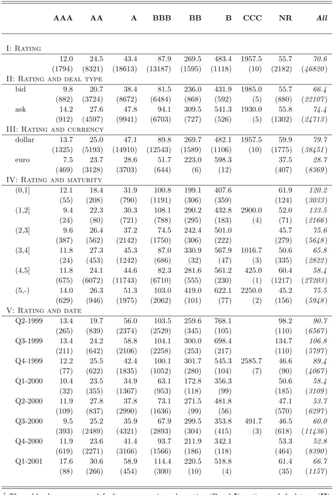
Since the empirical literature on credit default swaps is restricted to just one other study (Aunon-Nerin et al., 2002), it is interesting to look at the properties of the data first; see Table 1. Panel I subdivides the 46820 observations by the reference entity’scredit rating at the quote date. As may be expected, the rating is a very important determinant of default swap premiums as average premiums decrease monotonously with credit quality. In panel II, the sample is further subdivided by deal type. The number of bid quotes is roughly equal to the number of ask quotes. The average bid-ask spread is 8 bps, but an increasing pattern with ratings may be observed.9 _{Note that the bid-ask spreads are} relatively large compared to the quote size. For instance, for AA the average bid-ask spread of 6.8 bps amounts to 28% of the average quote of 43.4 bps. Contracts in our database are denominated in one of twocurrencies: either US dollars or euros. Panel III shows that dollar-denominated default swaps prevail, but recall that euro-denominated default swaps are only observed during the second half of the data period. For all ratings, dollar quotes are on average larger than euro quotes, except for rating B where the number of euro observations is rather small. This finding still holds, if we also control for quote date, though to a lesser extent (not shown here). The relation between premium level and contractmaturity is assessed in panel IV. Notice that more than 50% of the observations resides in the 4- to 5- year maturity range. There does not seem to be a clear relation between the average default swap premium and maturity. Our findings are in line with those of Aunon-Nerin et al. (2002), who tested several specifications for the maturity effect, but none of them appeared to be significant. Finally, panel V shows the behavior

9_{The bid-ask spread for CCC is negative, but this is most likely caused by the small number of}

of average premiums over time by grouping the default swaps by quote date into three-month periods. Except for AA and BB, the quotes for all ratings roughly follow a U-shape pattern over time: in the middle of the sample period, the average premium is lower than at the start and at the end.

6.2

Comparing Bond Spreads and Default Swap Premiums

To directly compare bonds and default swaps, we make the following intuitive argument. Suppose an investor in a coupon-bearing defaultable bond buys protection by entering into a credit default swap. The package consisting of the bond and the default swap is free of default risk, so we have “defaultable bond + default swap = default-free bond”. Hence, the default swap premium should be equal to the spread between the defaultable and the default-free bond.

To formalize our argument, consider a defaultable bond with coupon payment dates t = (t1, . . . , tn), coupon c, maturity tn and notional 1. Further, consider a default swap

with the same maturity, premium percentage P and notional 1. For simplicity, assume that the default swap’s and bond’s payment dates coincide. The valueV(t) of the package to the investor is given byv(t,t, c)−V¯(t,t, P) + ˜V(t), whose formulas are given by Equa-tions (2) to (4). We replace the integrals in the pricing formulas by the approximaEqua-tions from Section 4; the grids for both the bond and default swap are chosen to be equal to the payment dates t. Then

V(t) = n X i=1 p(t, ti)(c−P α(ti−1, ti))˜P(t, ti) + n X i=1 p(t, ti) ³ ˜ P(t, ti−1)−P(˜ t, ti) ´ +p(t, tn)˜P(t, tn).

‘insurance premium’ P α(ti−1, ti) on the default swap. The remaining terms shows that

the notional of 1 will be paid eventually, but that the timing depends on the occurrence of the credit event. The investor is thus protected against default risk, but is now exposed to the risk of prematurely receiving the notional and thus missing some of the promised coupons (prepayment risk).

If we further assume that the default-free and defaultable bond are priced at par, then their yields are equal to their coupon rates (ignoring the prepayment risk). Let y and

Y denote the yield of the defaultable and the default-free bond, respectively, then y =c

and Y =c−P, so that y−Y =P. This confirms that the bond spread should be equal to the default swap premium. However, we had to make several assumptions to get this result, so it is only approximately valid. Nevertheless, bond spreads and default swap premiums should be comparable. This relation was also presented by Aunon-Nerin et al. (2002), though without proof. Duffie (1999) showed that this relation holds exactly for par floating rate notes instead of fixed-income coupon bonds.

We will now determine to what extent this relation holds for our data set. For each quoted default swap written on an entity, we have to find a quoted bond issued by that same entity with the same maturity. Unfortunately, a bond with exactly the same ma-turity as the default swap is rarely available. Therefore, we examine two alternative methods:

1. Find a quoted bond whose maturity differs at most 10% from the default swap’s maturity;

2. Find two quoted bonds, one whose maturity is smaller than, but at most twice as small as, the default swap’s maturity, and one whose maturity is larger than, but at most twice as large as, the default swap’s maturity, and linearly interpolate their

spreads.

We call method 1 the matching method and method 2 the interpolation method. The performance of each method is evaluated for all three proxies for the default-free term structure.

Each time a pair can be formed of a default swap premium and a (matched or inter-polated) bond spread, we calculate two pricing errors.10 _{One by subtracting bond bid} spreads from default swap ask quotes, and the other by subtracting bond ask spreads from default swap bid quotes.11 _{The pricing errors are summarized in two ways. First, as} the average, denoted by the Mean Pricing Error (MPE), and second as the average of the absolute values, called the Mean Absolute Pricing Error (MAPE). A negative (positive) sign of the MPE statistic indicates that the bond market’s estimate of the issuer’s credit risk is larger (smaller) than the default swap’s market estimate. To test if this under-or overestimation is significant, we create a time series MPEi1, . . . ,MPEiS, where MPEit

denotes the mean pricing error for method i on date t. We then apply a one-sample Z-test (see e.g. Arnold, 1990, Chapter 11): Zi =

√

S·MPEi/si, where MPEi and si are

the sample mean and sample standard deviation of the MPEit series, respectively, and

S is the sample size. Asymptotically, Zi has a standard normal distribution. Similarly,

to determine if significant performance differences exist between our methods, we cre-ate a time series MAPEi1, . . . ,MAPEiS of mean absolute pricing errors for each method

i. Then, we use a paired Z-test (Arnold, 1990, Chapter 11) to determine if method i’s performance is significantly different from method j’s, while allowing for non-zero

corre-10_{The pricing error is often called the default swap basis by market participants; see O’Kane and}

McAdie (2001) and Hjort et al. (2002).

11_{In this way, we are comparing similar sides of the market. For instance, an investor can create an}

exposure to an issuer’s default by buying a bond – for which he pays the ask price – or by writing default swap protection – for which he receives the bid premium.

lation and unequal variances. The test statistic is defined as Zij =

√

S·d¯ij/sij, where

¯

dij and sij are the sample mean and sample standard deviation, respectively, of dijt =

MAPEit−MAPEjt, t= 1, . . . , S. Asymptotically, Zij has a standard normal distribution.

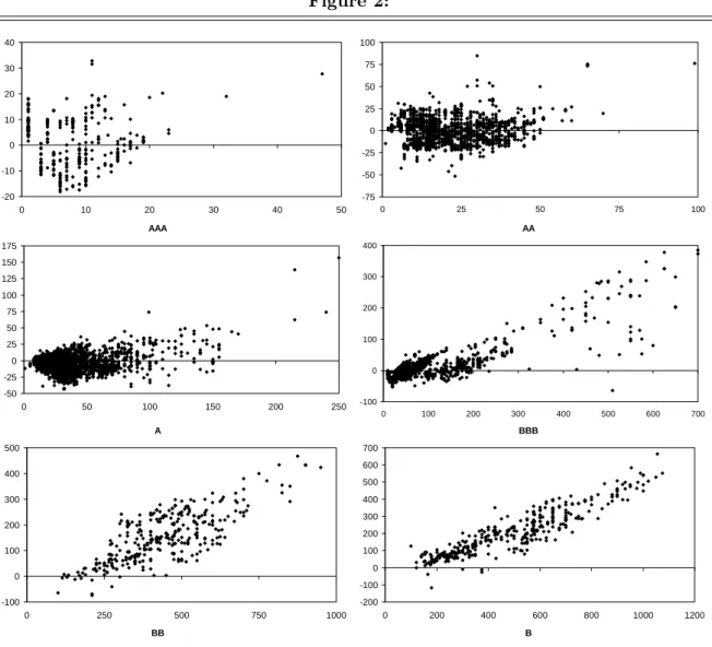
Figure 2 depicts scatter plots of pricing errors versus default swap premiums per rating for the interpolation method that uses the swap curve as default-free curve; the plots for the other methods are similar. If interpolated bond spreads over the swap curve are good estimates of default swap premiums, all points should lie on the horizontal axis. For ratings AAA, AA and A, this seems indeed to be the case, so that on average the method does a good job. This is confirmed by the MPE values in Table 2, which are approximately zero, though only for AAA insignificant. For rating BBB, the scatter plot and MPE statistic indicate that bond spreads are on average smaller than default swap premiums; for ratings BB and B this is almost always the case. Moreover, the Z-test indicates that the MPEs are significantly different from zero, so that for BBB, BB and B bond spreads are biased estimates of default swap premiums. For all ratings, the dispersion around the horizontal axis is fairly large: the MAPE statistics in Table 2, together with the average default swap premiums in Table 1, imply that the calculated premiums deviate on average 19% (for BBB) to 68% (for AAA) in absolute value from the market values.

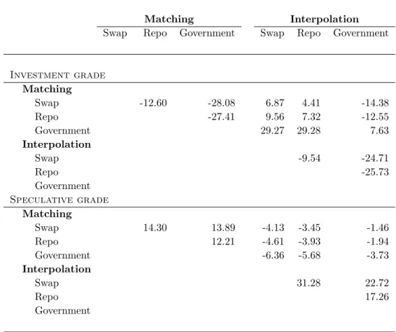
Tables 2 and 3 also shed light on the performance of the other methods. A striking result is the abominable performance of the government-based methods for AAA to A. Their MAPE values are up to four times higher than for methods that proxy the default-free curve with the swap or repo curve. As the paired Z-tests in Table 3 point out, the underperformance of the government curve for investment grade issuers (so including BBB too) is highly significant. Moreover, since the MPEs are negative, almost identical in size to the MAPEs and statistically significant, bond spreads relative to the government curve

are virtually always larger than default swap premiums for high grade issuers. The MPE values for the swap and repo curve methods are much closer to – but still significantly different from – zero. Looking at the MAPE statistics as well, the swap curve methods perform significantly better than the repo curve methods for investment grade, but signif-icantly worse for speculative grade entities. For speculative grade issuers, the government curve methods significantly outperform their swap- and repo-based counterparts. For all methods the MPE statistics take large, significantly positive values though, indicating that they all result in bond spreads being smaller than default swap premiums.

6.3

Estimating Hazard Functions

We now turn to the estimation of credit risk models as described in Section 4.4. We consider three proxies for the default-free curve – government, swap and repo curves – and three degrees for the integrated hazard function – linear, quadratic and cubic. For each issuer, we estimate all nine models for each day that we have at least one default swap quote and at least five bond quotes. Like in Section 6.2, this is done separately for the bid and ask sides of the market. A model’s quality at day t may be assessed by looking at the root mean squared error (RMSE) of the deviations between the market prices and the model prices

RMSE(t) = v u u t 1 b(t) b(t) X i=1 ei(t)2

where ei(t) = Pi(t)−v(t,ti, ci). A model’s RMSE is calculated as the average of its

RMSE(t) values over all days in the sample.

observe that the goodness of fit deteriorates as the rating declines. We further find that using more parameters (obviously) yields a better in-sample fit. This holds for all three proxies for the default-free curve, but especially for the government curve if we move from a linear to a quadratic model. Table 4 also indicates that using a cubic model has little advantage over a quadratic model for high grade bonds, but does fit better for low grade bonds. As to the choice of the default-free curve, we see that for the linear model, the government curve clearly underperforms the swap and repo curves. For quadratic and cubic models, on the other hand, choosing a proxy for the default-free curve is less important. Overall it seems sufficient for AAA and AA to use a linear model with a swap or repo curve, for A and BBB a quadratic model with a swap or repo curve, and for BB and B a cubic model with any default-free curve.

Now we turn to the discussion of the estimated coefficients of the integrated hazard function. For the constant hazard rate model, the average default intensity λ1 increases with the issuers’ credit rating, except that B’s is somewhat below BB’s. Therefore, on average, credit ratings do a good job in ranking firms by credit worthiness. However, the level of the default intensity differs considerably between the models, especially for investment grade bonds. For instance, if we use the swap curve, we would conclude that AAA’s default rate is only 7 bps, but if we use the government curve that number would be about ten times as large. In the quadratic integrated hazard model, the hazard function is linear, so that λ1 and λ2 are the level and slope coefficient of the hazard function, respectively. The estimates imply that if we compare the estimated spread curves of two ratings, the worst rating’s spread curve both starts at a higher level and is steeper. Again, noticeable differences exist between the three curves. Using the government curve, gives higher and steeper spread curves than using the swap curve. Comparing swap and repo

curves, we find that the levels differ by about 10 bps, just like in the linear model, but that the slopes are exactly equal.12 _{Finally, we look at the results of the cubic model.} Unlike the nicely ordered level and slope coefficients, there does not seem to be relation between λ3 and the credit rating. Interestingly, the λ3 parameters of the government curve models are almost equal to those of the swap and repo curve models.

In conclusion, the choice of a proxy for the default-free curve has a significant impact on the level and shape of the hazard function. Moreover, the fit of the model to investment grade bonds is better for the swap or repo curve than for the government curve. For speculative grade bonds, choosing a proxy is less important.

6.4

Comparing Model and Market Premiums

Having estimated a credit risk model for a specific issuer allows us to calculate model premiums of credit default swaps written on that issuer.13 _{Like above, we define two} pricing errors: as default swap ask quotes minus model premiums calculated from hazard functions estimated from bond bid quotes, and vice versa. Table 5 contains the MPEs and MAPEs for all nine models subdivided by rating, as well as one-sample Z-tests for the MPE statistics. Table 6 shows the outcomes of the paired Z-tests for the investment grade and speculative grade subsamples. If we compare these figures to the ones in Tables 2 and 3, we see very similar patterns. First, MAPEs increase with credit ratings for all models, except for high grade entities in the models that use the government curve. Second, government-based models perform very badly for investment grade issuers: their

12_{This simply reflects the construction of our repo curve as a parallel shift of the swap curve.}

13_{All premiums are calculated using euro proxies for the default-free term structure. Ideally, we}

should use dollar curves for dollar-denominated contracts, but we are unable to obtain dollar repo rates. However, repeating the analysis in this section for government and swap curves with dollar curves, gives very similar results (available on request from the authors): dollar-based and euro-based premiums have a correlation of over 99%.

MAPE statistics take significantly larger values than for swap- and repo-curve models, and their significantly positive MPE statistics indicate a large overestimation of default swap premiums. Third, the MPE values for the swap and repo curve models are close to zero, and for first degree swap models and second and third degree repo models mostly statistically insignificant. Fourth, for speculative grade bonds, the government curve models outperform the swap- and repo-based models; for quadratic and cubic models this outperformance is significant. Finally, for all models the MPE statistics take significantly positive values, indicating that they all underestimate the credit risk of low grade entities. Estimating a hazard rate model gives a clear improvement over the direct methods of Section 6.2. Comparing the best direct method to the best model for each default-free curve proxy, we find that MAPE statistics are reduced by 15% to 55% for investment grade issuers. For speculative grade issuers, hazard rate models outperform the direct methods by 15% to 20%. Even though using a model works better than directly comparing bond spreads and default swap premiums, the model premiums of the best-performing model still deviate on average 20% to 50% in absolute value from the market values. So the models fit rather well to bonds, but their ‘out-of-sample’ performance on default swaps is somewhat poor.

We now try to identify the best model. The results show that swap and repo models on average do a reasonable job for investment grade issuers. The swap-based models some-what underestimate the true default swap premiums, and except for the linear model, this bias is significant; the repo-based model, on the other hand, slightly overestimates the market premiums, but these differences are mostly insignificant (except for the linear model). Looking at the MAPE statistics as well, the linear and quadratic swap curve models significantly outperform their repo- and government-based counterparts for

in-vestment grade entities; the differences between swap and repo models are small though. For speculative grade issuers, the quadratic and cubic government curve models signifi-cantly work better than swap and repo models with equal degrees. As to the choice of the optimal degree of the integrated hazard function, the pairedZ-tests indicate that the quadratic model works significantly better than, or not significantly different from, the linear and cubic models. This result holds for both investment grade and speculative grade issuers. All in all, a quadratic model that uses the repo curve seems to be the best choice for investment grade issuers: it gives unbiased estimates, and has the second lowest MAPE values. For speculative grade entities, none of the considered models can be recommended, since they all significantly underestimate credit risk.

The underestimation of default swap premiums for speculative grade issuers is sub-stantial. If an investor would like to exploit this difference between bond and default swap markets, he has to write default swap protection (receiving the high default swap premium) and short a bond (paying the low bond spread). However, as noted earlier in Section 2, shorting corporate bonds is typically unfeasible, so that positive pricing er-rors can persist in the market. An explanation for these pricing erer-rors may be found in missing features in the bond and/or default swap pricing models. O’Kane and McAdie (2001) and Hjort et al. (2002) discussed a large number of factors that may affect the difference between default swap and bond markets. They mentioned that for speculative grade issuers, the delivery option in physically settled default swaps (see Section 2) is particularly important: for higher default probabilities, it is more likely that the default swap will be triggered, and the protection buyer actually has to deliver obligations to the seller. The delivery option will thus be more valuable for low grade issuers.14 _{Since the}

delivery option is not taken into account in our default swap pricing model in Section 4.2, the pricing error can be used as a rough estimate of the value of the delivery option. Hence, if the delivery option is truly an important missing factor, pricing errors should be positively correlated with hazard rates. If we calculate the correlation of pricing errors from the linear integrated hazard model with ˆλ1, we get values between 35% and 47%, depending on the proxy for the default-free curve.

6.5

Analyzing Pricing Errors

In the previous section, we showed that the MAPE increases if the credit rating deterio-rates. It is also interesting to see if differences between market and model premiums can be related to other characteristics than the issuer’s credit rating. We try to accomplish this by regressing absolute pricing errors on dummy variables for the following charac-teristics: deal type (bid or ask), currency (euro or dollar), rating (AAA, AA, A, BBB, BB), maturity (1-year intervals up to 5 years, and an interval from 5 to 10 years) and quote date (6-month periods). For each set of dummies, the categories are mutually ex-clusive, so that an identifying restriction is required. We set a linear combination of the coefficients to 0, where the weight of a coefficient is equal to the sample mean of the cor-responding dummy variable.15 _{The advantage of imposing these restrictions over setting} one coefficient to zero is that the constant of the regression equals the sample mean of the dependent variable. Furthermore, each coefficient can be interpreted as the change in the absolute pricing error for that dummy for an otherwise representative observation.

Table 7 shows the regression results for the quadratic specification of the integrated option: for a default swap written on an issuer with an annual default probability ofλ and a potential gain ofGof switching from an expensive to a cheaper deliverable, the value is approximatelyλG.

15_{For instance, ifβ andαdenote the coefficients of the bid and ask dummies, we imposebβ+aα= 0,}

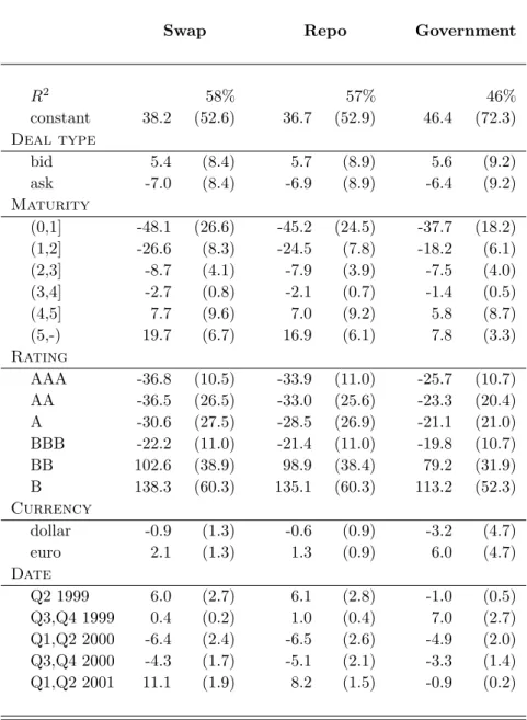
hazard function for all three proxies for the default-free curve; the results for the linear and cubic model are similar. We observe that most parameters are statistically different from zero, the signs of the parameters are largely consistent between the models and the R2 values are between 46% and 58%. Mispricings strongly differ between deal types as errors on bid quotes are larger than on ask quotes. The maturity of the default swap contract is also predictive of the pricing error, since the coefficients of the maturity dummies are sig-nificant (except for the interval from 3 to 4 years) and monotonously increasing. Likewise, the coefficients of the rating dummies are highly significant and monotonously increas-ing. The currency dummies are only significant for the government model, indicating that the swap- and repo-based models price dollar- and euro-denominated default swaps similarly. Finally, the parameters for thequote date dummies show that for most models pricing errors in 2000 were smaller than in 1999 or 2001, although not all coefficients are statistically significant.

7

Summary

In this paper, we empirically investigated the market prices of credit default swaps. We showed that a simple reduced form model priced credit default swaps better than directly comparing bonds’ yield spreads to default swap premiums. The model worked reasonably well for investment grade issuers, but quite poor in the high yield environment; so, there is definitely room for more empirical research and further model development. Further, we found evidence that government bonds are no longer considered by the markets to be the reference default-free instrument. Swap and/or repo rates have taken over this position. We also showed that bond spreads and default swap premiums are relatively insensitive

to changes in the assumed constant recovery rate as long as the hazard function is scaled accordingly.

Acknowledgements

This paper is a revised and abridged version of our earlier paper ’An Empirical Compari-son of Default Swap Pricing Models’. The earlier version was presented at the Tinbergen Institute 2001 Econometrics Workshop in Rotterdam, the 2002 Meeting of the European Financial Management Association (EFMA) held in London, the 2002 Meeting of the European Finance Association (EFA) held in Berlin, the 2nd T.N. Thiele Symposium on Financial Econometrics in Copenhagen and Forecasting Financial Markets 2003 held in Paris. The authors thank attendants of these seminars and Kees van den Berg, Mark Dams, Andrew Gates, Albert Mentink, Zara Pratley, Micha Schipper, Martijn van der Voort and two anonymous referees for valuable suggestions and critical remarks. The authors also thank Rabobank International for providing the data. Financial support by the Erasmus Center for Financial Research (ECFR) is much appreciated. Views ex-pressed in the paper are the authors’ own and do not necessarily reflect those of Rabobank International, ABN Amro or Robeco Asset Management.

References

Aonuma, K. and Nakagawa, H. (1998), Valuation of credit default swap and parameter estima-tion for Vasicek-type hazard rate model, Working paper, University of Tokyo.

Arnold, S. F. (1990), Mathematical Statistics, Prentice Hall, New Jersey.

Aunon-Nerin, D., Cossin, D., Hricko, T. and Huang, Z. (2002), Exploring for the determinants of credit risk in credit default swap transaction data: Is fixed-income markets’ information sufficient to evaluate credit risk?, Working paper, HEC-University of Lausanne and FAME.

url: http://www.hec.unil.ch/dcossin/PAPERS.HTM

Bakshi, G., Madan, D. and Zhang, F. (2001), Understanding the role of recovery in default risk models: Empirical comparisons and implied recovery rates, Working paper, University of Maryland.

url: http://papers.ssrn.com/sol3/papers.cfm?abstract id=285940

BBA (2001),BBA Repo Rates, British Bankers’ Association.

url: http://www.bba.org.uk/

BBA (2002),Credit Derivatives Report 2001/2002, British Bankers’ Association.

url: http://www.bba.org.uk/

Black, F. and Scholes, M. (1973), ‘The pricing of options and corporate liabilities’, Journal of Political Economy81, 637–654.

Brooks, R. and Yan, D. Y. (1998), ‘Pricing credit default swaps and the implied default proba-bility’,Derivatives Quarterly 5(2), 34–41.

Chan, K., Karolyi, G. A., Longstaff, F. A. and Sanders, A. B. (1992), ‘An empirical comparison of alternative models of the short-term interest rate’,Journal of Finance47(3), 1209–1227. Collin-Dufresne, P. and Solnik, B. (2001), ‘On the term structure of default premia in the swap

and LIBOR markets’,Journal of Finance 56(3), 1095–1115.

Culp, C. L. and Neves, A. M. P. (1998), ‘Credit and interest rate risk in the business of banking’,

Derivatives Quarterly4(4), 19–35.

Cumby, R. E. and Evans, M. D. (1997), The term structure of credit risk: Estimates and specification tests, Working paper, Georgetown University and National Bureau of Economic Research.

url: http://www.georgetown.edu/faculty/evansm1/wpapers.htm

Das, S. R. and Sundaram, R. K. (2000), ‘A discrete-time approach to arbitrage–free pricing of credit derivatives’,Management Science46(1), 46–62.

Driessen, J. (2001), The cross-firm behaviour of credit spreads, Working paper, Tilburg Univer-sity.

url: http://www1.fee.uva.nl/fm/PEOPLE/Driessencv.htm

Duffee, G. R. (1998), ‘The relation between Treasury yields and corporate bond yield spreads’,

Journal of Finance53(6), 2225–2242.

Duffie, D. (1996), ‘Special repo rates’,Journal of Finance 51(2), 493–526.

Duffie, D. (1999), ‘Credit swap valuation’,Financial Analysts Journal(January–February), 73– 85.

Duffie, D. and Huang, M. (1996), ‘Swap rates and credit quality’,Journal of Finance51(3), 921– 949.

Duffie, D., Pedersen, L. H. and Singleton, K. J. (2003), ‘Modeling sovereign yield spreads: A case study of Russian debt’,Journal of Finance58(1), 119–160.

Duffie, D. and Singleton, K. J. (1997), ‘An econometric model of the term structure of interest-rate swap yields’,Journal of Finance52(4), 1287–1321.

Duffie, D. and Singleton, K. J. (1999), ‘Modeling term structures of defaultable bonds’,Review of Financial Studies12(4), 687–720.

D¨ulmann, K. and Windfuhr, M. (2000), ‘Credit spreads between German and Italian sovereign bonds: Do one-factor affine models work?’, Canadian Journal of Administrative Sciences 17(2).

Fr¨uhwirth, M. and S¨ogner, L. (2001), The Jarrow/Turnbull default risk model: Evidence from the German market, Working paper, Vienna University of Economics.

url: http://www.wu-wien.ac.at/usr/abwldcf/mfrueh/publ.html

Fr¨uhwirth, M. and S¨ogner, L. (2003), The implicit estimation of default intensities and recov-ery rates, in ‘Proceedings of the 64th Scientific Conference of the Association of University Professors of Management 2002’, Munich.

Geyer, A., Kossmeier, S. and Pichler, S. (2001), Empirical analysis of European government yield spreads, Working paper, Vienna University of Economics.

url: http://www.wu-wien.ac.at/usr/or/geyer/publ.htm

Golub, B. and Tilman, L. (2000), ‘No room for nostalgia in fixed income’,Risk(July), 44–48. Greene, W. H. (2000), Econometric Analysis, 4th edn, Prentice Hall, New Jersey.

Harrison, M. and Pliska, S. (1981), ‘Martingales and stochastic integrals in the theory of con-tinuous trading’,Stochastic Processes and Their Applications 11, 215–260.

Hjort, V., McLeish, N. A., Dulake, S. and Engineer, M. (2002), The high beta market - Exploring the default swap basis, Fixed Income Research, MorganStanley, London.

Hull, J. and White, A. (2000), ‘Valuing credit default swaps I: No counterparty default risk’,

The Journal of Derivatives8(1), 29–40.

dis-counts implicit in debt prices’,The Journal of Risk5(1).

Jarrow, R. A., Lando, D. and Turnbull, S. M. (1997), ‘A Markov model for the term structure of credit spreads’,Review of Financial Studies 10(2), 481–523.

Jarrow, R. A. and Turnbull, S. M. (1995), ‘Pricing derivatives with credit risk’, Journal of Finance50(1), 53–85.

Jarrow, R. A. and Turnbull, S. M. (1998), Credit risk,in C. Alexander, ed., ‘Handbook of Risk Management and Analysis’, John Wiley & Sons, pp. 237–254.

Jarrow, R. A. and Turnbull, S. M. (2000), ‘The intersection of market and credit risk’,Journal of Banking & Finance24, 271–299.

Keswani, A. (2000), Estimating a risky term structure of Brady bonds, Working paper, Lancaster University.

url: http://www.lums2.lancs.ac.uk/ACFIN/Papers/2000.HTM

Koci´c, A., Quintos, C. and Yared, F. (2000), Identifying the benchmark security in a multifactor spread environment, Fixed Income Derivatives Research, Lehman Brothers, New York. Litterman, R. and Iben, T. (1991), ‘Corporate bond valuation and the term structure of credit

spreads’,Journal of Portfolio Management (Spring), 52–64.

Longstaff, F. A. (2000), ‘The term structure of very short-term rates: New evidence for the expectations hypothesis’,Journal of Financial Economics 58(3), 397–415.

Longstaff, F. A. and Schwartz, E. S. (1995), ‘Valuing credit derivatives’,Journal of Fixed Income

(June), 6–12.

Madan, D. B. and Unal, H. (1998), ‘Pricing the risks of default’,Review of Derivatives Research 2, 121–160.

Journal of Finance29(2), 449–469.

Nakagawa, H. (1999), Valuation of default swap with affine-type hazard rate, Working paper, University of Tokyo.

Nielsen, S. S. and Ronn, E. I. (1998), The valuation of default risk in corporate bonds and interest rate swaps, Working paper, University of Copenhagen and University of Texas at Austin.

url: http://www.math.ku.dk/∼nielsen/

O’Kane, D. and McAdie, R. (2001), Explaining the basis: Cash versus default swaps, Fixed Income Research, Lehman Brothers, London.

Patel, N. (2003), ‘Flow business booms’,Risk (February), 20–23.

Perraudin, W. and Taylor, A. (1999), On the consistency of ratings and bond market yields, Working paper, Bank of England and Birkbeck College.

url: http://wp.econ.bbk.ac.uk/respap/respap frames.html

Sch¨onbucher, P. J. (2000), A LIBOR market model with default risk, Working paper, University of Bonn.

url: http://www.schonbucher.de/

Scott, L. (1998), A note on the pricing of default swaps, Working paper, Morgan Stanley Dean Witter.

Taur´en, M. (1999), A comparison of bond pricing models in the pricing of credit risk, Working paper, Indiana University, Bloomington.

Figure 1: (a) (b) (c) 10 11 12 13 14 15 0 0.2 0.4 0.6 0.8 1 recovery rate d e fa u lt sw a p p re m iu m ( b p s) 0.0 0.2 0.4 0.6 0.8 1.0 1.2 0 0.2 0.4 0.6 0.8 1 recovery rate % 0.00 0.05 0.10 0.15 0.20 %

1–recovery rate hazard rate (1–recovery) · hazard 2.5% 3.0% 3.5% 4.0% 4.5% 0 1 2 3 4 5 6 7 8 9 10 maturity z e ro -c o u p o n r a te 10% 30% 50% 70% 90%

Figure 2: AAA AA A BBB BB B -20 -10 0 10 20 30 40 0 10 20 30 40 50 -75 -50 -25 0 25 50 75 100 0 25 50 75 100 -50 -25 0 25 50 75 100 125 150 175 0 50 100 150 200 250 -100 0 100 200 300 400 0 100 200 300 400 500 600 700 -100 0 100 200 300 400 500 0 250 500 750 1000 -200 -100 0 100 200 300 400 500 600 700 0 200 400 600 800 1000 1200