BoostingTree: Parallel Selection of Weak Learners in
Boosting, with Application to Ranking
Levente Kocsis · Andr´as Gy¨orgy · Andrea
N. B´an
Received: / Accepted:
Abstract Boosting algorithms have been found successful in many areas of ma-chine learning and, in particular, in ranking. For typical classes of weak learners used in boosting (such as decision stumps or trees), a large feature space can slow down the training, while a long sequence of weak hypotheses combined by boost-ing can result in a computationally expensive model. In this paper we propose a strategy that builds several sequences of weak hypotheses in parallel, and extends the ones that are likely to yield a good model. The weak hypothesis sequences are arranged in a boosting tree, and new weak hypotheses are added to promising nodes (both leaves and inner nodes) of the tree using some randomized method. Theoretical results show that the proposed algorithm asymptotically achieves the performance of the base boosting algorithm applied. Experiments are provided in ranking web documents and move ordering in chess, and the results indicate that the new strategy yields better performance when the length of the sequence is limited, and converges to similar performance as the original boosting algorithms otherwise.
Keywords Boosting·Random search·Ranking
1 Introduction
Boosting algorithms (Schapire 2002) have been found successful in many areas of machine learning and, in particular, in ranking (Burges et al 2011). For typical classes of weak learners used in boosting (such as decision stumps or trees), a large feature space can slow down the training considerably. A natural way to accelerate Levente Kocsis·Andrea N. B´an
Data Mining and Web search Research Group, Informatics Laboratory, Institute of Computer Science and Control, Hungarian Academy of Sciences (MTA SZTAKI)
E-mail: [email protected], [email protected] Levente Kocsis
E¨otv¨os Lor´and University Andr´as Gy¨orgy
Department of Computing Science, University of Alberta E-mail: [email protected]
the training is to limit the set of features accessible to the weak learner at certain decision points. For example, when the weak learner attempts to create a decision stump, the selection of feature is limited to a subset of all features (or even to one particular feature). Such, an approach was followed by Busa-Fekete and K´egl (2009, 2010) using multi-armed bandit algorithms (see, e.g., Auer et al 2002a,b) to narrow the freedom of the weak learners.
Another drawback of boosting algorithms is that in order to improve on the performance of individual weak learners, such algorithms tend to cumulate a long sequence of (weak) hypotheses resulting in a computationally expensive model. This problem is exacerbated when bandit algorithms are used to speed up the training, since the exploring nature of bandit algorithms will include much weaker hypotheses, and a larger number of these are needed to achieve similar perfor-mance. One way to avoid the inclusion of poor hypotheses in the final ensemble is to revisit some of these decisions later. In this way effectively a tree of weak hypotheses (and their combination weights) is built, where, for any node, the path from the root to the node determines a weighted sequence of hypotheses. The number of possible children of a node is determined by the number of possible next hypotheses to be chosen. While a standard boosting algorithms just selects a hypothesis in each step, here first a node (a leaf or an inner node that does not have the maximum number of children) has to be selected, and then a weak hypothesis extending the hypothesis sequence leading to this node.
The above procedure essentially runs several (dependent) boosting algorithms in parallel. This idea is very similar to improving local search algorithms by having run several search instances in parallel. The latter problem is discussed in our pre-vious paper (Gy¨orgy and Kocsis 2011). There we proposed an efficient algorithm, calledMetaMax, that dynamically starts instances of a local search algorithm and allocates resources to the instances based on their (potential) performance. The major difference between the two problems is that in our current set-up new se-quences are created from old ones, instead of starting each algorithm instance from scratch, introducing serious inter-dependence between the different boosting runs. Furthermore, the boosting methods considered must differ to produce different hypothesis sequences. Therefore, constraints on selecting the next weak hypothe-sis in each node at each time instant are necessary. In this paper, we propose a new algorithm,BoostingTree, that borrows the core ideas behind selecting the promising algorithm instances from theMetaMaxalgorithm, and adapts them to the tree-based structure of hypotheses sequences.
While the proposed algorithm can be of interest in many applications of ma-chine learning, ranking problems are particularly suited for this approach. First, in many ranking problems, such as web search or move ordering in games, a fast model is essential. Moreover, the ranking evaluation measures are notoriously non-smooth, therefore virtually all learning algorithms optimize a different measure, and combining these algorithms with a strategy that ’corrects’ their decisions when alternative decisions could improve performance with respect to the ’real’ evaluation measure should only improve their performance.
The rest of the paper is organized as follows. Section 2 summarizes related research. The proposed algorithm is described in Section 3, while theoretical con-siderations are given in Section 3.1. Simulation results on web search benchmarks and move ordering in chess are described in Section 4. Conclusions and future work are provided in Section 5.
2 Related work
The importance of restricting the number of hypotheses combined by boosting was noted by Margineantu and Dietterich (1997), proposing several methods to achieve this including early stopping, pruning techniques that aim to diversify the hypotheses included in the final model (such as Kappa pruning), and the Reduce-Error pruning that greedily adds hypotheses (from the larger pool) to reduce error on a pruning (or validation) set. While the boosting pruning problem was proven to be NP-complete by Tamon and Xiang (2000), several algorithms have been proposed to select a small set of hypotheses from a larger ensemble (see e.g. Mart´ınez-Mu˜noz et al 2009; Tsoumakas et al 2009 for an overview). It is worth noting that most of the pruning algorithms are more effective when the ensembles are created by bagging rather than boosting, although the latter provides a natural ordering of the hypotheses (Mart´ınez-Mu˜noz et al 2009).
A more effective way of achieving good performance in boosting with a re-duced number of hypotheses is throughl1 regularization of the weights attached to hypotheses, combined often with early stopping. This approach was chosen by, for example, Xi et al (2009); Xiang and Ramadge (2009). While we believe that l1 regularization can improve boosting algorithms for ranking problems as well, adjusting these algorithms are out of the scope of this paper (moreover, such reg-ularization can be used in addition to theBoostingTreealgorithm as well) and therefore we do not attempt to compare the proposed algorithm to these tech-niques. For simplicity, we restrict our attention in the experimental work to early stopping for limiting the number hypotheses, while keeping in mind that alterna-tive approaches can improve any of the tested algorithms.
Accelerating the training of boosting algorithms was discussed by Escudero et al (2000) proposing several algorithms, including LazyBoost that reduces the set of features considered in each iteration to a random subset. Busa-Fekete and K´egl (2009) improved on this algorithm by posing the feature selection as a multi-armed bandit problem, and using the bandit algorithmUCB(Auer et al 2002a) to focus the selection on more informative features while keeping some exploration in the process. Since, the selection of features in subsequent boosting iterations is non-stationary, Busa-Fekete and K´egl (2010) argued for the more sensible use of adversarial bandit algorithms such asExp3(Auer et al 2002b). The latter will be revisited in Section 4.
As we mentioned before, theBoostingTreealgorithm is based on the Meta-max algorithm (Gy¨orgy and Kocsis 2011), an algorithm specifically designed to speed up local search algorithms by running several search instances in paral-lel. Therefore, it is natural to consider the alternatives toMetamaxdiscussed by Gy¨orgy and Kocsis (2011) as alternatives toBoostingTreeas well. In particular, the bandit based approach by Streeter and Smith (2006) could be used to alternate between boosting sequences, however, it is not clear how to adapt the algorithm beyond selecting amongst sequences with a fixed start-up (such as varying the ini-tial model). Luby et al (1993) proposed an anytime algorithm that, in our context, would translate to running (possibly randomized) boosting algorithms repeatedly and stopping them after a prescribed number of iterations (that varies from in-stance to inin-stance). While the algorithm would produce a plethora of hypothesis sequences with varying length, some randomization needs to be introduced in the boosting algorithm, otherwise all sequences would be just prefixes of the longest
sequence. If, in the spirit of the experiments described by Gy¨orgy and Kocsis (2011), the sequences would vary only in the initial model that would limit the improvement potential on later hypotheses.
The allocation strategy of theMetamaxalgorithm is inspired by theDIRECT
optimization algorithm of Jones et al (1993). Recently, Munos (2011) provided a generalization of theDIRECTalgorithm, called the simultaneous optimistic opti-mization (SOO) algorithm. Both algorithms are designed to find the optimum of a smooth function, without knowledge of the actual smoothness. In order to do so, the algorithms build a search tree, partitioning the input space, where each leaf node represents a set from the actual partition. Since the selection mecha-nism of theMetaMaxalgorithm is based on that of theDIRECT algorithm, the mechanism of Munos (2011) could also be used to improve MetaMax, and by association, the BoostingTree algorithm. While theDIRECT and theSOO al-gorithms build trees, just likeBoostingTree, an important difference is that the former algorithms build full trees, while theBoostingTreeadds the children of a node one by one.
While multi-armed bandit approaches to boosting have been discussed above, it could be interesting to look at tree based variants of the bandit algorithms, such asUCT(Kocsis and Szepesv´ari 2006). Some of our preliminary empirical analysis (not reported in this paper) indicated thatUCTwould spend too much effort in getting the first few hypotheses right (a natural behavior for games, where the move in the current position has to be decided), and too little attention is paid to subsequent weak learners that can have the same influence in the combined performance. Nested Monte-Carlo search (Cazenave 2009) has been applied to one-player games, and could be used for the same purpose as theBoostingTree
algorithm, but we leave the analysis of these Monte-Carlo algorithms for future research.
Another approach that builds a tree of alternatives is the alternating decision tree (ADT) algorithm (Freund and Mason 1999). While bothADT and Boost-ingTree are applied to boosting, a major difference is that while in ADT the constructed tree is one model, in our approach the leaves of the tree are individual models.
3 The BoostingTreealgorithm
In this paper we consider speeding up boosting algorithms. Given a set of instances X, the goal of a boosting algorithm is to create a model M :X →R from weak hypotheses (generated by weak learners) wj ∈ W, where W ⊂ {w : X → R} is a set of weak hypotheses. Each x ∈ X is usually described by a feature vector, and with a slight abuse of notation the feature vector representingxwill also be denoted byx. The goal of constructing the model can be any supervised learning task; in this paper we will be concerned about creating models for ranking. The modelM is built iteratively in a linear fashion from the weak hypotheses: a model M is an ensembleM =Pl(M)
j=1 wj, wherel(M) is the number of weak hypotheses used in constructingM, which will often be referred to later as the ’length of the boosting sequence’, and in each step of the algorithm a weak hypothesis wj is added to the existing model. While typically a model is aweighted combination of weak hypotheses, to simplify the notation we assume that the weight is already
included in the hypotheseswi in the above formulation. The selection of the next hypothesis depends on the current modelM, the training dataD, and optionally on a constraintC that restricts the new weak hypothesis to be an element of a restricted setWC⊆ W. Thus, one step of the boosting algorithmA encapsulates the reweighting of the data, the computation of a hypothesis by the weak learner (subject to the constraint), and the weighting of the hypothesis. That is, if the actual model isMi=Plj=1wj, the next weak hypothesis selected by the standard boosting algorithm iswi+1 =A(Mi, D).
As mentioned before, a single step of boosting algorithms may be speeded up by imposing some constraint on the next weak hypothesis. Given a constraint Ci, the constrained boosting algorithmAselects the next weak hypothesiswi+1= A(Mi, Ci, D) (the unconstrained version can be described in this way asA(Mi,∅, D)). A typical case is when the weak hypotheses are decision stumps (depending only on a single feature of the observations), and the constraintCi selects a single feature: then the stepA(Mi, Ci, D) is nothing but optimizing a weak learnerwi+1over the set of decision stumps corresponding to the feature selected byCi. We denote the measure of the performance of the modelM with dataDbyf(M, D). Throughout this paper this measure will typically be some ranking measuref(M, D) =V(M, D) that evaluates the modelM on the particular datasetD, but the provided method works for any other performance measure. Since it is possible that the performance of a model is decreased by adding more weak hypotheses, we also define the func-tion ˆfto be the maximum of the ranking measure over the possible prefixes of an ensemble, that is,
ˆ f(M) = max 0≤j≤l(M)f 0 @ j X i=1 wi, D 1 A.
While standard boosting algorithms typically produce a deterministic sequence of weak learners (for a given dataD), allowing several different constraint values for each model leads to a tree: the edges of the tree correspond to (weighted) weak hypotheses, while any node in the tree is a model that sums the hypotheses that are on the path from the root to the node. Assuming constraintsC1, . . . , Ck can be selected at a node M, the children ofM correspond to the weak hypotheses {A(M, Ci, D)}i=1,...,k as edges. Assuming the available constraints at each node are fixed in advance, the tree can be built in several ways. In this section we propose an algorithm, called BoostingTree, that provides a systematic way of exploring the tree. The key component ofBoostingTreeis the way it selects the nodes (i.e., the models) to extend with a new hypothesis. Before describing this selection mechanism, we first revisit theMetaMaxalgorithm (Gy¨orgy and Kocsis 2011) that forms the basis of the selection procedure.
The goal of theMetaMaxalgorithm is to find a maximizerx∗ of a functionf,
using a given local search algorithm. As we discussed in the introduction, Meta-Maxruns several instances of the local search algorithm in parallel, and allocates in every step additional resources to the most promising instances. The key idea of MetaMaxis the assumption of bounding the convergence of the local search instances by a function cg(n), where n is the number of steps taken by the lo-cal search algorithm,gis typically an exponential function, andc is an unknown constant. The algorithm then steps every local search instance that has the high-est optimistic bound (the actual bhigh-est value plus the confidence boundcg(n)) on the performance for some particular range of values of c. The idea behind the
algorithm, first introduced in the context of Lipschitz optimization without the knowledge of the Lipschitz constant (Jones et al 1993), is that if the convergence rate g(n) is only known up to a constant factor, then instead of selecting an ar-bitrary value of this constant, all algorithms are considered that are optimal for some values of the constant. As the functiongis also unknown, it is replaced by a sequence of functions{hr}chosen such that it aids the convergence of the
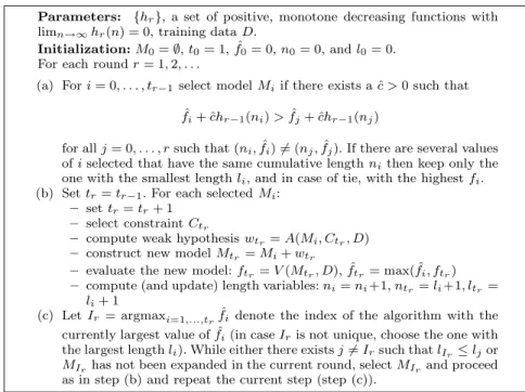
Meta-Maxalgorithm. TheMetaMaxalgorithm is shown in Figure 1, for completeness. At the beginning of each round r, a new instance is created randomly (instance Ar), and the most promising instances are selected in step (b), whereni denotes the number of steps made byAi, ˆfi is its current estimate of the optimum, and
ˆ
fi+ ˆchr(ni) is the optimistic estimate on the performance ofAiwith assumed con-vergence rate ˆchr(n) (note that bothni and ˆfi may change from round to round). The selection procedure will be explained in more details in the context of the
BoostingTree algorithm. The most promising algorithms are selected and used to make another step. Finally, in step (c’), it is ensured that the instance with the currently best estimate of the optimum makes the most steps. While introducing this step does not have much effect in practice (typically, if the best algorithm is not the one with the most steps, its step number would increase very quickly in short rounds, even without (c’)), it helps the algorithm in certain pathological cases, and also aids its theoretical analysis (see Gy¨orgy and Kocsis 2011 for a more detailed discussion).
The boosting tree algorithm employs this idea in the node selection procedure. Nodes (models) are added to the tree in rounds. In each roundr, for each node Mi already added to the tree, the performance ofMi is evaluated as ˆfi= ˆfi(Mi), and an estimate of the potential performance of extendingMi is formed as
ˆ
fi+ ˆchr(ni) (1)
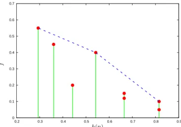
wherehris some decreasing positive function (typically exponential) andniis the cumulative length ofMi, which is defined as the sum of the length of the modelMi and the number of children ofMialready in the tree. Then the algorithm expands those nodes which maximize the performance estimate (1) for some values of ˆc. While it may seem that almost all models will be selected in this way (for different values of ˆc), it is easy to see that exactly those models are selected that lie on the corners of the upper convex hullHof the set of points{(hr(ni),fˆi)}∪{(0,maxifˆi)} where iranges over all modelsMi that are already in the tree, see Figure 2 (the reason for this is that ˆfi+ ˆc(hr(ni)−x) is a tangent line ofH ifi maximizes (1) for ˆc).
Thinking of a sequence of weak hypotheses as a local search algorithm, the above selection rule for leafs is the same as that of the MetaMaxalgorithm, as for leaf nodes the cumulative length is exactly the number of hypotheses in the corresponding model. For internal nodes some adjustment needs to be made to avoid excessive attention to models that are hard to improve: Note that for many local search algorithms, including boosting, there are situations when the current model can only be improved slightly or cannot be improved at all by a single step. Then, ifhr sufficiently prefers lower complexity models (i.e., ensembles that are sums of fewer hypotheses), and we considered the model length instead of the cumulative length, a hardly improvable model would typically be selected if at least one of its children were selected. Our solution to this problem is to introduce the notion of cumulative length of a node, which is the length of the path to the
MetaMax: A multi-start strategy with infinitely many algorithm instances.
Parameters: {hr}, a set of positive, monotone decreasing functions with
limn→∞hr(n) = 0. For each roundr= 1,2, . . .
(a) Initialize algorithmArby choosing uniformly random starting pointXi,0,
evaluatingf(Xi,0), and by settingnr= 0,fˆr=f(Xi,0).
(b) Fori= 1, . . . , r−1 select algorithmAiif there exists a ˆc >0 such that ˆ
fi+ ˆchr−1(ni)>fˆj+ ˆchr−1(nj)
for allj = 1, . . . , r−1 such that (ni,fˆi)6= (nj,fˆj). If there are several values ofi selected that have the same step number nithen keep only one of these that has the smallest index.
(c) Step each selectedAiobtaining the sample pointXi,ni, and update
vari-ables. That is, for each selectedAi, setni=ni+ 1, evaluate f(Xi,ni) and iff(Xi,ni)>fˆithen set ˆXi=Xi,ni,fˆi=f(Xi,ni).
(c’) LetIr = argmaxi=1,...,rfˆi denote the index of the algorithm with the currently largest estimate off∗(in caseI
ris not unique, choose the one with the smallest number of stepsni). IfIr 6=Ir−1, step algorithmAIr
(nIr−1−nIr+ 1) times and setnIr=nIr−1+ 1, and ˆfIr andXIr as the
largest value offand its location, respectively, encountered by algorithm
AIr.
(d) Estimate the location of the maximum with ˆXr= ˆXIrand its value with
ˆ
fr= ˆfIr.
Fig. 1 TheMetaMaxalgorithm. The algorithm attempts to maximize a real-valued function
f(X) with the help of local search instances Ai that differ in their initial point Xi,0. The
algorithm allocates further time to instances that appear more promising (step (b) and (c)) and gives high priority to instances that suddenly provide the best estimate having being less promising previously (step (c’)). New instances are started in every round (step (a)).
node plus the number of children of the node. Intuitively, this modification yields that the probability of expanding a child of a node (even with a higher potential than other far descendants, grandchildren and more) decreases as more and more children of a given node are expanded.
The BoostingTree algorithm is shown in Figure 3. Note that for a model Mi,li denotes the depth of the corresponding node, the cumulative (or extended) length ni is the depth plus the number of children already generated,fi is the actual performance of the model, ˆfi is the performance of the best ancestor ofMi. Furthermore,tr−1 is the number of models in the tree generated before round r. Note that, unlike to theMetaMaxalgorithm, most values defined in the algorithm are static, and only the cumulative length variablesni depend implicitly onr, for example,fi and ˆfi remain unchanged once nodeiis created.
The algorithm starts with an empty tree, and in every phase expands the nodes that have the potential of leading to the highest performing model (step (a)). For each selected node, a constraint is set on the weak learners and the selected node is extended by a new hypotheses according to the boosting algorithm. The variables of the selected node and the new node are updated according to step (b). The final step (c) enforces after each iteration that we expand the model
0 0.1 0.2 0.3 0.4 0.5 0.6 0.7 0.2 0.3 0.4 0.5 0.6 0.7 0.8 0.9 h(n) ˆf
Fig. 2 Selecting models for expansion inBoostingTree: the points represent the models,
and the models that lie on the corners of the upper convex hull (drawn with dashed blue lines) are selected.
with best ranking measure until it leads to the longest path in the tree, an idea also borrowed from theMetaMaxalgorithm. Although this last step usually does not influence strongly the algorithm, it slightly speeds up the convergence when a new and shorter ‘leader’ is found (in fact, if such a step would not be present such an ‘overtake’ would be followed by very short phases, until the leading path is expanded for a sufficient number of times). Furthermore, this step helps to handle some pathological situations, and simplifies the theoretical analysis of the algorithm.
Note that one could also try to approach the problem by running several in-stances of a boosting algorithm independently (with some randomization or with a diverse set of constraints applied for the different runs) to obtain efficient models. Then, for example, one could run these instances in parallel, and use the Meta-Maxalgorithm to select which instances should be continued. However, such an approach would neglect the strong correspondence between the different runs. Tak-ing into account these correspondences leads to the tree structure and the Boost-ingTreealgorithm described above. One can, of course, runMetaMaxover runs of different boosting algorithms (including even BoostingTree), but this is an orthogonal issue and is beyond the scope of the present paper.
3.1 Some theoretical results
In this section we provide some basic properties of theBoostingTreealgorithm, following the analog analysis for the MetaMax algorithm (Gy¨orgy and Kocsis 2011). First note that the base boosting algorithmA used insideBoostingTree
would provide a sequence of modelsMrA=Mr−1+A(Mr−1,∅, D), r= 1,2, . . .(with M0 =∅), thus, in each iteration of the algorithm, the model is augmented with a weak hypothesis computed without any constraints. It is reasonable to expect that ourBoostingTree algorithm can mimic the performance of A if a node is
Parameters: {hr}, a set of positive, monotone decreasing functions with limn→∞hr(n) = 0, training dataD.
Initialization:M0=∅,t0= 1, ˆf0= 0,n0= 0, andl0= 0.
For each roundr= 1,2, . . .
(a) Fori= 0, . . . , tr−1 select modelMiif there exists a ˆc >0 such that ˆ
fi+ ˆchr−1(ni)>fˆj+ ˆchr−1(nj)
for allj= 0, . . . , rsuch that (ni,fˆi)6= (nj,fˆj). If there are several values ofiselected that have the same cumulative lengthnithen keep only the one with the smallest lengthli, and in case of tie, with the highestfi. (b) Settr=tr−1. For each selectedMi:
– settr=tr+ 1
– select constraintCtr
– compute weak hypothesiswtr=A(Mi, Ctr, D) – construct new modelMtr=Mi+wtr
– evaluate the new model:ftr=V(Mtr, D), ˆftr= max( ˆfi, ftr) – compute (and update) length variables:ni=ni+1,ntr=li+1, ltr=
li+ 1
(c) Let Ir = argmaxi=1,...,trfˆi denote the index of the algorithm with the
currently largest value of ˆfi(in caseIris not unique, choose the one with the largest lengthli). While either there existsj6=Irsuch thatlIr≤ljor
MIrhas not been expanded in the current round, selectMIrand proceed
as in step (b) and repeat the current step (step (c)).
Fig. 3 TheBoostingTreealgorithm.
expanded sufficiently many times, that is, a sufficiently rich set of constraints are used in the selection process. The following assumption ensures this property.
Assumption 1 For any node M of the BoostingTree assume that the node can have only finitely many children, each defined by a different constraint, such that for one of these constraints, C, we have A(M, C, D) =A(M,∅, D).
It is easy to see by induction that the above assumption implies that the full infinite boosting tree (where each node has its maximum number of children) contains all the modelsMrAgenerated by the boosting algorithmAsuch thatMrA+1 is a child ofMrA, for eachr= 0,1,2, . . ..
Furthermore, notice that the selection procedure (a) implies that a modelMi with the smallest step numberni is always selected (for the largest values of ˆc). Since each node can have only a finite number of children, for any n there is a bounded number of nodes in the tree whose step number can be at most n (if a node at depth l can have at mostk children, then its step number is always at mostl+k). This implies that each node of the infinite boosting tree is expanded by a maximum number of times if BoostingTree is run for a sufficiently long time.
The above two facts imply the following consistency result:
Theorem 1 Suppose Assumption 1 holds. Then any modelMrAgenerated by the orig-inal boosting algorithmAis also generated by theBoostingTreealgorithm if it is run
for a sufficiently long time. As a consequence, the asymptotic training performance of
BoostingTreeis at least as good as that ofA:limr→∞fˆ(MIr)≥limr→∞fˆ(M
A r).1 The goal ofBoostingTree is to find the best model possible on the training data. Since it is not clear which constraints are going to be the most relevant, the algorithm tries to explore several paths in the boosting tree while keeping the most promising ones as long as possible (in an ideal setting the algorithm would explore just the optimal path, spending all resources on it, not wasting effort on suboptimal combinations of weak hypotheses).
The trade-off in this exploration-exploitation problem can be best analyzed by evaluating the length ofMIr, that is, how many weak hypotheses are combined in
MIr at the end of roundr. Note thatMIr is the longest extension of the actually
best model of the boosting tree (which is typically also the actually best model); therefore we will refer to MIr as the best leaf-model of the tree. The following
theorem shows that the length lIr of MIr is of the order of the square root of
tr, the total number of times a weak hypothesis is computed inBoostingTree (note that the number of nodes in the tree is tr+ 1). The proof of this result is a straightforward modification of that of Theorem 15 of (Gy¨orgy and Kocsis 2011). Note that in practice we have found that the BoostingTree algorithm behaves better in the sense that the length ofMIr is typically much larger, about
Ω(tr/lntr); for more details see Section 4.7.
Theorem 2 At the end of any round r the number of weak hypotheses in the best leaf-modelMIr is between rand2r. That is,
r≤nIr =lIr <2r. (2) Furthermore, nIr =lIr≥ √ 2tr+ 7−1 2 . (3)
Proof The first statement of the lemma is very simple, since in any round the length of the best leaf-model increases by either one or two: If the best leaf-model is expanded in roundr according to step (a) and it remains the best-leaf model then triviallynIr =nIr−1+1. If the best leaf model is expanded but another model becomes better during the round, then the latter model is expanded so many times that the corresponding leaf-model (which, in turn, will becomeMIr) be of depth
nIr=lIr=lIr−1+ 2. Finally, ifMIr−1 is not expanded according to step (a), then the length ofMIr has to be set tolIr−1+ 1. Thus
1≤nIr−nIr−1 =nIr−nIr−1≤2
in all situations. Since in the first round clearly exactly one node of the boosting tree is generated, that is,nI1 = 1, (2) follows.
To prove the second part, notice that in any roundr, at mostnIr−1+ 1 nodes can be expanded according to step (a) as no algorithm can be used that has taken more steps than the currently best one (and hence the currently best leaf-node). Also, no extra weak hypotheses have to be computed if the conditions in step (c) are met. If not, then at mostnIr−1+ 1 weak hypotheses have to be computed in
0 0.1 0.2 0.3 0.4 0.5 0.6 0.7 0.8 0 0.1 0.2 0.3 0.4 0.5 0.6 0.7 0.8 feature 2 feature 1 +
-Fig. 4 Synthetic binary classification problem with two features. The positive data points are
marked with +, and the negative points with−.
addition (i.e., the best model has to be extended with at most this many weak hypothesis). Therefore,
tr≤tr−1+ 2nIr−1+ 2. Thus, since step (c) has no effect in round 1, we obtain
tr≤1 + r X s=2 2(nIs−1+ 1). Then, by (2) we have tr≤1 + 4 r X s=2 s= 1 + 2(r+ 2)(r−1)≤1 + 2(nIr+ 2)(nIr−1) which yields (3). 3.2 An illustrative example
We illustrate the BoostingTree algorithm on a synthetic binary classification problem combined with the AdaBoost algorithm (Freund and Schapire 1997) with decision stumps. The classification problem is shown in Figure 4. A stump w:R→Ris defined by a split of the real line represented by a half lineH and a weightv such thatw(u) =vifu∈H andw(u) =−vifu6∈H. The constraints at the nodes restrict the choice of the stumps to a single feature. Denoting the feature selected for the stumpwj byij, and theith coordinate of a feature vectorx∈ X by xi, the model after l steps becomesMl(x) =Plj=1wj(xij), and the classifier
decides to class + ifM(x)≥0, and to class−otherwise.
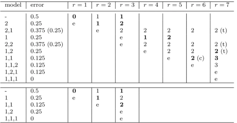
The model generated on this problem by a regular AdaBoost algorithm is shown in Table 1, left. While the model classifies all data points correctly, it includes five decision stumps, and perfect classification can be obtained with only three decision stumps as shown in Table 1, right, if we split always feature 1. A similarly small model can be obtained by splitting three times feature 2.
In each step of theAdaBoostalgorithm, first, the data are re-weighted, then a decision stump is chosen (a feature and a split for that feature is selected), and a
Table 1 Models for the synthetic classification problem. The left table shows the sequence of decision stumps generated by a regularAdaBoostalgorithm with the corresponding weigths. For each decision stump, the top row specifies the feature to be splitted, and the second row specifies the interval for which positive label is assigned. The table on the right specifies the model generated if in each step the decision stump is constrained to feature 1. For this model, if we sum the weights over the intervals, we have +0.55−0.55−0.80 =−0.8 if feature 1 is less than 0.2 (thus negative label), +0.8 between 0.2 and 0.4 (positive),−0.3 between 0.4 and 0.6 (negative), and +0.8 above 0.6 (positive).
feature 1 2 2 1 1 split ≤0.4 ≤0.4 >0.6 >0.2 >0.6 weight 0.55 0.55 0.62 0.76 0.67 feature 1 1 1 split ≤0.4 >0.6 >0.2 weight 0.55 0.55 0.80
weight is computed for the decision stump. When theBoostingTreealgorithm is combined withAdaBoost, it selects a model (a combination of decision stumps) to be extended, and selects the feature to be added to the model. The latter is the constraint on the construction of the new weak hypothesis (i.e., the decision stump to be added). The re-weighting of the data, the selection of the split, and the formula for the weight of the new decision stump remains unchanged from the
AdaBoostalgorithm.
Two possible runs of theBoostingTreealgorithm are shown in Table 2. The differences in the possible runs are due to the different selection of the features for the new decision stumps (which is the same as the selection of the constraint in step (b) of the algorithm; cf. Figure 3). Normally, the selection is done by selecting randomly from the features that has not been expanded for the model chosen for expansion in step (a). In the worst case scenario of Table 2, top, instead of random, the feature that least likely to lead to a small optimal model in the algorithm is selected. While for the best case scenario of Table 2, bottom, the feature that leads more likely to such a model is selected.
As shown in Table 2, theBoostingTreealgorithm starts with an empty model (the first row in each table). In each round, the ‘active’ models2are considered for expansion with their error (1−fˆ) and cumulative length (n). Of these candidate models, only those are expanded that obey the properties outlined in step (a) of the BoostingTree algorithm. In this discussion we will not make the functions hr more specific since, due to the simplicity of the considered problem, the steps shown in the tables would be independent of the choice ofhr as long as it obeys the specified requirement (i.e., being positive, monotone decreasing function). To understand better how the selection works, consider the candidates in round 3 of the top table, the empty model, the model that includes a decision stump with feature 2, and the model with the feature sequence (2,1). The empty model that has cumulative length equal to 1 (it has model length equal to 0, and has been expanded once) will be selected for expansion since the inequality holds for large ˆc (e.g., for ˆc=∞). For the other two candidate models the inequality holds for small values of ˆc(e.g., for ˆc= 0), but both have the same valuen= 2, and according to the description of the algorithm, we select for expansion only the one with smaller model length. Subsequently the empty model is extended with feature 1 (fourth row), given that it was already extended with feature 2. Similarly, the model with
2 Active models are those that have been evaluated already and have not been expanded
Table 2 BoostingTreeruns combined withAdaBooston the synthetic problem of Figure 4. The separate runs are provided for a worst case (top) and a best case scenario (bottom). Each row corresponds to a feature sequence, that is, to the model obtained withAdaBoost by sequentially constraining the decision stumps in the ensemble with the particular feature from the sequence. The first row in each table corresponds to an empty model. In the error column classification error corresponding to the obtained model (i.e., feature sequence) is given (the error equals 1−f), while the minimum error (1−fˆ) over the prefixes of the particular sequence is given in brackets if differs fromf. In the columns corresponding to the consecutive rounds (r) the cumulative length (n) is provided. The number is given in bold if the sequence is selected for extension. The letterespecifies the round in which the sequence is evaluated,c
is attached if the sequence is extended due to step (c) of theBoostingTreealgorithm, while the lettertmarks a tie situation. When a sequence is extended with both features, it will not be considered for further expansion, and, therefore, the corresponding cell in the table is left empty for the following rounds.
model error r= 1 r= 2 r= 3 r= 4 r= 5 r= 6 r= 7 - 0.5 0 1 1 2 0.25 e 1 2 2,1 0.375 (0.25) e 2 2 2 2 2 (t) 1 0.25 e 1 2 2,2 0.375 (0.25) e 2 2 2 2 (t) 1,2 0.25 e 2 2 2(t) 1,1 0.125 e 2(c) 3 1,1,2 0.125 e 3 1,2,1 0.125 e 1,1,1 0 e - 0.5 0 1 1 1 0.25 e 1 2 1,1 0.125 e 2 1,2 0.25 e 1,1,1 0 e
the single feature 2 is extended with the same feature 2. For both models the
AdaBooststeps follow, thus the data is reweighted, the split is computed for the added feature, the model is augmented with the new decision stump (consisting of the feature and the split), and the new model is evaluated.
Considering how well the BoostingTree algorithm performs on this classi-fication problem, we observe that even in the worst case, the number of steps necessary to obtain a 0-error model for theBoostingTreealgorithm is not much higher than for the regular AdaBoost (nine vs. five), with the BoostingTree
yielding a smaller model (three decision stumps instead of five). Moreover, even in this case the number of times a split has to be selected is smaller for the Boost-ingTreecombination (nine) compared to how many times the regularAdaBoost
looks for a split (ten, since in each step the split is computed for both features). In the best case scenario, only four steps are needed to find the smallest 0-error model.
Looking at some finer details of theBoostingTreeruns, in particular the one corresponding to the worst case scenario, we note that step (c) of the algorithm is activated in the sixth round. In this case, it does not alter the course of the algorithm since the (1,1) sequence would have been the only one to be selected anyway, but it would have given a further push if more complex models (with larger lengthl) had been generated previously, which is favorable since exactly this model
was extended subsequently to the optimal model. In the seventh round there is a tie broken based on the classification error of the model, with the sequence (1,2) having the smallestf. Ties with identical ˆf andnoccurred also in round 3 and 5, and were broken according to the smallest length (l). Finally, in a somewhat more favorable scenario the sequence (2,2) could be extended to the alternative smallest 0-error model, which is (2,2,2). This is an example for the situation of the error first increasing and then decreasing mentioned in Section 3.
3.3 Implementation issues
Note that, as shown in the example in the previous section, the training error becomes zero exponentially fast in boosting algorithms. However, when the labels are noisy, it is typically worth to run the training longer, and set the actual number of training iterations using a validation set. When the BoostingTree includes several models with optimal performance on the training set, the shortest models are selected, and the optimal models are grown at the same rate, building a full tree from any optimal node. One can avoid this, for example, by using a validation set to compute ˆfi. Note however, that we have not encountered such situations in our experiments.
Boosting algorithms work by weighting the data points, and, in order to reduce the computation time, most implementations take advantage of the possibility to compute incrementally the weights of the data points, and store some auxiliary record for each point as the algorithm proceeds. In the case of AdaBoost, the auxiliary records consist of the current weights and, for the ranking algorithms discussed in Section 4.3, they consist of the current score of each document. Since a boosting tree can be expanded at any node, in order to use the same speed-up technique, one would need to keep the auxiliary records for each node of the boosting tree, which may result in prohibitive memory consumption. It is clear that for nodes corresponding to short boosting sequences, recomputing these records is sufficiently fast, and there is no real need to store such auxiliary records. To balance between memory usage and computation time, one can develop heuristics to store the records for the most promising and/or most recently used models only, and recompute them for other models when necessary. In the experiments, presented in the next section, we have simply decided to always recompute the weights; since most of the tree is shallow (we aim for short models in any case), this has not introduced a large computational overhead, and the observable speed-ups include this overhead.
4 Experiments
In this section we describe the empirical evaluation of theBoostingTreealgorithm using two boosting algorithms for ranking:LambdaMART(Section 4.3.1) and ND-CGboost(Section 4.3.2). The two boosting algorithms are used either standalone (we refer to these as the standard variants), combined with adversarial bandits (Exp3.P; Busa-Fekete and K´egl 2010), or combined with the BoostingTree al-gorithm. Thus in total we have six algorithms. The evaluation measure used in the experiments is the Normalized Discounted Cumulative Gain (NDCG; J¨arvelin
and Kek¨al¨ainen 2000), described in Section 4.1. Two standard webpage ranking benchmark datasets are used for evaluation (Section 4.4 and Section 4.5), with an additional benchmark constructed with move ordering in chess (Section 4.6). The section ends with a discussion on the results and some observations regarding how
BoostingTreebehaves in practice.
4.1 Ranking measure: NDCG
NDCG is one of the most popular measures to evaluate ranking, and has been used in several ranking challenges (see, e.g., Chapelle and Chang 2011). Here we consider a typical ranking problem, where documents should be provided to answer queries. We denote the set of queries byQ={q1, . . . , qn}. For each queryqi, a ranker is faced with a set ofmidocumentsDi={di1, . . . , dimi}. Each document
dij is labeled by a number lij indicating its relevance with respect to the ith query. The gain of a document is typically defined asgij= 2lij−1, with irrelevant documents being labeled 0, and more relevant ones having higher valued labels (1,2,3, . . .). Faced with a queryqi, a ranking algorithm outputs a permutationπ of the documents, with πik denoting the document ranked on the kth position, and conversely,rij denotes the rank of the documentdij.
The Discounted Cumulative Gain (DCG) of theith query is usually defined up toK documents as follows: DCG@Ki(π) = min(K,mi) X k=1 γk giπik,
whereγk is a discount factor. J¨arvelin and Kek¨al¨ainen (2000) defines the discount factor byγk= 1, ifk= 1, andγk= 1/log2k, otherwise. This definition is used by the benchmark described in Section 4.4, while the benchmark of Section 4.5 uses a slightly different definition, withγk = 1/(log2(k+ 1)) that results in a strictly decreasing discount sequence (as opposed to the first definition, whereγ1=γ2).
LetmaxDCG@Ki= maxπDCG@Ki(π) denote the discounted cumulative gain corresponding to an optimal ranking for theith query. Then normalized discounted cumulative gain (NDCG) of theith query is defined as
N DCG@Ki(π) = DCG@Ki(π)
maxDCG@Ki
, and the average NDCG is defined by
N DCG@K(π) = 1 n n X i=1 N DCG@Ki(π).
Finally,M eanN DCG(π) is defined as the average of the normalized discounted cumulative gain up to the number of documents:
M eanN DCG(π) = 1 n n X i=1 1 mi mi X k=1 N DCG@ki(π)
Both ranking measures,N DCG@K(π) andM eanN DCG(π), need to be max-imized. They reach their maxima at 1, for an optimal ranking, and are always non-negative as the lowest value forgiπik is assumed to be non-negative.
4.2 Algorithms
In this section we revisit the two boosting algorithms used in the experiments, and some details of the specific implementation of BoostingTree and Exp3.P
algorithms are also given.
In a typical ranking problem documents related to a query have to be ordered, and each query-document pair is described by a feature vector. Since a model obtained by a boosting algorithm returns a real valued score for each pair, the ordering for a particular query is obtained by sorting the documents according to their scores.
The two boosting algorithms for ranking used in the experiments ( Lamb-daMARTandNDCGboost) apply trees as weak hypotheses (regression and deci-sion trees, respectively). When selecting a weak hypothesis, the tree construction algorithms build a tree by recursively partitioning the input space and assigning a value (or label) to each leaf. When a partition corresponding to a node is being subpartitioned, the tree construction algorithm selects a feature, and partitioning is made by thresholding this feature value. The feature and the corresponding threshold in each internal node, as well as the label of each leaf is selected to minimize some measure, such as the mean squared error for regression trees.
In our algorithms the selection of the weak learner, a regression or decision tree, is often constrained. In these experiments we choose to use constraints that allow partitioning a node of a tree based on a single feature, and the constraint determines for each node which feature should be used. Thus a constraint can be seen as a tree of features, where each node in the constraint tree restricts the choice of feature in the corresponding internal node of the decision tree. The leaves in the decision tree hold the labels for a particular subpartition, and have no corresponding node in the constraint tree. It may happen that a tree construction algorithm decides not to split the data further at some node (for instance, when only one document falls in the node), then some elements of the constraint tree are ignored.
Next we specify details concerning the algorithms applied in the experiments. 4.2.1 TheBoostingTreealgorithm
There are two important details that have to be specified when implementing the
BoostingTree algorithm: selecting appropiate functions forhr and chosing how to set constraints on the weak learners. For the former, we opted to the functions hr(n) =e−n/
√
tr, successfully applied in (Gy¨orgy and Kocsis 2011).
The constraint tree is constructed by selecting features randomly for all nodes. The size of the tree depends on how large the decision tree to be used in the base boosting algorithm is intended to be. In practice, the constraints on each node can be selected during the construction of the decision tree. When expanding a particular model, constraint trees that have been already selected for that model are not repeated.
4.2.2 TheExp3.Palgorithm
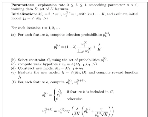
TheExp3.Palgorithm is an algorithm originally designed for multi-armed bandit problems (Auer et al 2002b). The use of the algorithm to improve the speed of a
Parameters: exploration rate 0 ≤ λ ≤ 1, smoothing parameter η > 0, training dataD, set ofKfeatures.
Initialization:M0=∅,t= 1,ω(1)k = 1, with k=1,. . . ,K, and evaluate initial
modelfo=V(M0, D)
For each iterationt= 1,2, . . .
(a) For each featurek, compute selection probabilitiesp(kt):
p(kt)= (1−λ) ω (t) k P k′ω (t) k′ + λ K.
(b) Select constraintCt using the set of probabilitiesp(kt). (c) compute weak hypothesiswt=A(Mt−1, Ct, D). (d) Construct new modelMt=Mt−1+wt
(e) Evaluate the new model: ft =V(Mt, D), and compute reward function ˜
ft
(f) For each featurek, computeρ(kt),ωk(t+1):
ρ(kt)= 8 < : ˜ ft p(kt) if featurekis included inCt 0 otherwise ω(kt+1)=ωk(t)exp λ 3K ρ (t) k + η p(kt)√K !!
Fig. 5 TheExp3.Palgorithm applied for boosting.
boosting algorithm was proposed by Busa-Fekete and K´egl (2010). The algorithm applied for boosting is described in Figure 5. Note that the description differs somewhat from that of Busa-Fekete and K´egl (2010) in the initialization of the weightsω(1)k , however the algorithm performs exactly the same way independently of the initial values of the weights as long as they are equal. Moreover, in step (f) of the original algorithm, η is divided by the square root of the maximum iteration number. We absorbe this into the smoothing parameter η in order to simplify notation.
There are several variants proposed by Busa-Fekete and K´egl (2010) on how to select the constraint in step (b). In our implementation, the constraint is similar to the one described in Section 4.2.1 for theBoostingTreealgorithm, except that features are not selected uniformly at random, but according to the probability distribution p(kt). If the weak hypotheses are decision stumps this choice of the constraint is very similar to the multi-armed bandit set-up. For decision trees with several nodes, the choice of the constraint is less trivial. Busa-Fekete and K´egl (2010) discussed several choices, and decided in their empirical evaluations for a similar approach to ours. This is perhaps the simplest approach without having to solve a more complicated credit assignment problem over the involved features.
A further choice has to be made on the reward function ˜ft. When combined with AdaBoost Busa-Fekete and K´egl (2010) suggested the use of a function based on the edge of the weak hypothesis. For the boosting algorithms for ranking
discussed in Section 4.3, this is a less natural choice. Experimentally we found that the difference ˜ft=ft−ft−1is an appropiate choice in our case. In Section 4.4 we revisit this issue in a short discussion.
Altough we tested several values of the constantsλandη, we have not noticed any strong influence on the performance, except for some extreme values (such as λ= 1 orλ= 0). Therefore all reported experiments withExp3.Pare withλ= 0.3 andη= 0.1.
4.3 Boosting algorithms
Next we describe the two boosting algorithms used in our ranking problems.
4.3.1 TheLambdaMARTalgorithm
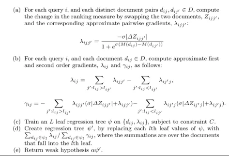
LambdaMART (Wu et al 2010) is a gradient tree boosting algorithm that ap-proximates the gradient of the ranking measure by combining a pairwise gradient, based on the scores given by the generated model, and the change in the rank-ing measure when two documents are swapped. Empirically, this approximation was shown to be close to the true gradient inLambdaRank(Donmez et al 2009).
LambdaMARTis one of the most successful ranking algorithm, forming the core of the winning entry at the Yahoo! learning to rank challenge (Burges et al 2011). One iteration of theLambdaMARTalgorithm that represents the computation of a weak hypothesis given the current model is shown in Figure 6. The standard version of the algorithm starts with an initial model (possibly empty as in our implementation), and iteratively adds new weak hypotheses. No constraints are placed on the generation of the regression tree (step (c)), in this variant. When called from theBoostingTreeor theExp3.Palgorithm, the selection of features is constrained in the manner discussed above.
In the experiments, we optimize forN DCG, thus, the change in the ranking measure,∆Z, after swapping documentsdij anddij′ becomes
∆N DCGijj′ = 1
n maxDCGi
(γrij−γrij′)(gij−gij′).
The combination coefficientαin the algorithm is set to 0.2, which appears to be a good choice for all three benchmarks, although the value was selected only after a few test runs.σis set to 1, while the number of leavesLvaries with the problem, depending mostly on the size of the data, but, as we discuss in Section 4.6, also on the complexity of the features.
When analyzing the time complexity ofLambdaMART, we can split the algo-rithm into two parts: (1) the computation ofλij andγij, and (2) the training the regression tree. The first part scales linearly with the product of the number of documents and the number of documents per query (the latter term can be smaller if there are only a few relevant documents for each query). The second part scales linearly with the product of the number of documents, the number of leaves, and the number of features considered in each internal node. If the number of leaves is small and, more importantly, the selection in an internal node is constrained to one particular feature, then the first part may dominate the computation time, otherwise the second part can be far more expensive.
Parameters: current model M, training data D, constraint C, ranking measureZ, constantsσ, α >0, number of leavesL.
(a) For each queryi, and each distinct document pairsdij, dij′ ∈D, compute the change in the ranking measure by swapping the two documents,Zijj′, and the corresponding approximate pairwise gradients,λijj′:
λijj′= −
σ|∆Zijj′| 1 +eσ(M(dij)−M(dij′))
(b) For each queryi, and each documentdij∈D, compute approximate first and second order gradients,λijandγij, as follows:
λij= X j′:lij>lij′ λijj′− X j′:lij<lij′ λij′j, γij=− X j′:lij>lij′
λijj′(σ|∆Zijj′|+λijj′)− X
j′:lij<lij′
λij′j(σ|∆Zij′j|+λij′j). (c) Train anLleaf regression treeψon{dij, λij}, subject to constraintC. (d) Create regression tree ψ′, by replacing each lth leaf values of ψ, with
P
dij∈ψlλij/
P
dij∈ψlγij, where the summations are over the documents
that fall into thelth leaf. (e) Return weak hypothesisαψ′.
Fig. 6 Computing the weak hypothesis in theLambdaMARTalgorithm.
4.3.2 TheNDCGboostalgorithm
NDCGboost(Valizadegan et al 2009) is a boosting algorithm that optimizes the expectation of NDCG over all possible permutations of documents. The computa-tion of a weak hypothesis given a current model in theNDCGboostalgorithm is provided in Figure 7. The binary classifier used in step (b) of the algorithm is a de-cision tree withL leaves, where the numberL varies with the problem (similarly as in the case of LambdaMART). The constraint imposed on the tree building algorithm is also similar to the constraint imposed in LambdaMART, with the standard NDCGboost iteratively adding unconstrained weak hypotheses, while the BoostingTree and theExp3.P algorithms constrain every added tree by a feature tree. Although we are not aware of any strong performance obtained in any ranking challenge with NDCGboost, the main reason it is included in our experiments is that it appears to us as a highly performing ranking algorithm, which is also illustrated in Sections 4.4 and 4.5.
When analyzing the time complexity ofLambdaMART, we can split the algo-rithm into three parts: (1) the computation ofγij, (2) the training of the decision tree (assumed to be the classifier), and (3) the computation of the combination weight. The first and third parts scale linearly with the product of the number of documents and the number of documents per query (and as for LambdaMART, the latter term can be smaller if there are only a few relevant documents for each query). The second part scales linearly with the product of the number of docu-ments, the number of leaves, and the number of features considered in each internal node. Similarly toLambdaMART, the first and third parts take a significant time
Parameters: current modelM, training dataD, constraintC.
(a) For each queryi, and each document pairdij, dij′ ∈Di,j6=j′, compute
θijj′, and the weightγijfor each documentdj∈Dj, as follows:
θijj′ = eM(dij)−M(dij′) “ 1 +eM(dij)−M(dij′)”2 γij= mi X j′=1:j′6=j 2lij−2lij′ maxDCGi θijj′.
(b) Train a binary classifierψthat maximizesPn i=1
Pmi
j=1γijψ(dij), subject to constraintC.
(c) Compute the combination weightα:
α= 1 2log2 0 B @ Pn i=1 P j,j′:ψ(dij)<ψ(dij′)θijj′ 2lij−1 maxDCGi Pn i=1 P j,j′:ψ(dij)>ψ(dij′)θijj′ 2lij−1 maxDCGi 1 C A.
(d) Return weak hypothesisαψ.
Fig. 7 Computing the weak hypothesis in theNDCGboostalgorithm.
compared to the second part only if the number of leaves is small and in the pres-ence of a strong constraint (when the optimization in the training of the decision tree is rather limited, e.g., when the tree is constrained by a feature tree).
4.4 The LETOR benchmark
The LETOR benchmark collection3 is perhaps the most frequently used bench-mark dataset for learning to rank. One of the most significant feature of LETOR is that the results of several reference algorithms are available for the datasets included. For our experiments we selected the largest dataset, MQ2007, from the Letor 4.0 collection, which is 46 dimensional, with 1692 queries and 69,623 doc-uments (thus, approximately 41 docdoc-uments/query in average), and is split in five folds. The relevance labels are ranging from 2 (most relevant) to 0 (irrelevant). On this dataset theRankBoost (Freund et al 1998) algorithm has roughly the best results out of the algorithms enlisted on the website associated with the bench-mark collection, and therefore, in the following we also show the performance of
RankBoost as a baseline (note that the standard performance measure for this dataset isM eanN DCG).
On this dataset, for bothLambdaMARTandNDCGboostsmall decision trees with only 2 leaves appeared to be a good choice for the weak learners, thus, in fact, we use stumps. For learning withExp3.P accelerated boosting, the reward function for theExp3.Palgorithm has to be defined. In the experiments we used the change in N DCG on the training set (after adding a new weak hypothesis)
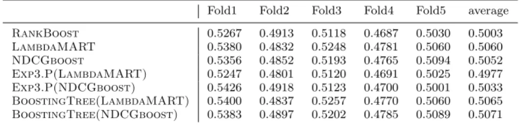
Table 3 M eanN DCGon the MQ2007 dataset from the Letor 4.0 benchmark collection for the five folds, and their average. TheRankBoostresults are provided as baseline on the LETOR website. For each fold, the best model for the standard variant of theLambdaMARTand the
NDCGboostalgorithms is selected based on theM eanN DCGon the validation set in 1,000 iterations (i.e., ensembles of at most 1,000 hypotheses), and in the table the M eanN DCG
of the selected model on the corresponding test set is reported. Similarly, theM eanN DCG
on the test sets for theExp3.Pvariants correspond to the ensembles with the best validation
M eanN DCGin 5,000 iterations, while forBoostingTreeit corresponds to the best validation
M eanN DCGof the first 5,000 hypothesis sequences.
Fold1 Fold2 Fold3 Fold4 Fold5 average
RankBoost 0.5267 0.4913 0.5118 0.4687 0.5030 0.5003 LambdaMART 0.5380 0.4832 0.5248 0.4781 0.5060 0.5060 NDCGboost 0.5356 0.4852 0.5193 0.4765 0.5094 0.5052 Exp3.P(LambdaMART) 0.5247 0.4801 0.5120 0.4691 0.5025 0.4977 Exp3.P(NDCGboost) 0.5426 0.4918 0.5123 0.4700 0.5001 0.5033 BoostingTree(LambdaMART) 0.5400 0.4837 0.5257 0.4770 0.5060 0.5065 BoostingTree(NDCGboost) 0.5383 0.4897 0.5202 0.4785 0.5089 0.5071
as the reward. Using changes in M eanN DCG gave similar results, while using quantities related to the training of the weak classifiers as rewards fared worse. Finally,BoostingTreeoptimizes forM eanN DCGon the training set.
For this problem there is only one decision stump for each weak hypothesis, and the number of documents for each query is in the same order as the dimension of the data, while a quarter of the documents are relevant, therefore, for both boosting algorithms the time required for building the tree does not dominate outright the running time of the other steps of the respective boosting algorithm. In our implementation, bothExp3.PandBoostingTreewere approximately five to ten times faster per iteration than the standard variants.4Consequently, we run these two algorithms for five times more iterations then the standard variants.
TheM eanN DCGperformance on the five folds for the six algorithms are pro-vided in Table 3, in addition to the RankBoost baseline, while the N DCG@k performance are shown in Figure 8. Overall, the standard variants of both
Lamb-daMART and NDCGboost performed better than RankBoost, while the
dif-ference between the two standard variants is negligible.Exp3.P performs poorly when combined withLambdaMARTand somewhat worse than the standard vari-ant when combined with NDCGboost. BoostingTree performs slightly better than the corresponding standard algorithms, with a more pronounced improve-ment over NDCGboost, which might be related to the fact thatExp3.P is also more successful in this combination (on this dataset, randomized moves appear more successful withNDCGboost).
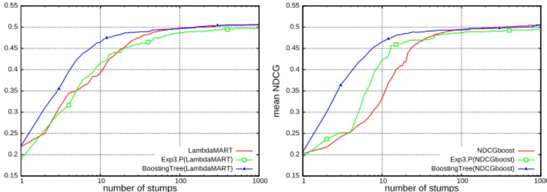
The M eanN DCGperformance of the six algorithms is shown in Figure 9 for varying limitations on the length of the boosting sequence. Note that the length
4 We discussed, so far, only the time complexity of the various components of the boosting
algorithms. Selecting the models to expand in a round of theBoostingTreealgorithm (Fig-ure 3, step (a)) takes more time than computing the probabilities in the Exp3.Palgorithm (Figure 5, step (f) and (a)), however, for all datasets described in the paper, these take still considerably less time than the reweighting of the data in either of the two boosting algorithms, that is, inLambdaMART(Figure 6, step (b)) and inNDCGboost(Figure 7, step (a)).
0.39 0.4 0.41 0.42 0.43 0.44 0.45 0.46 1 2 3 4 5 6 7 8 9 10 NDCG@k k LambdaMART Exp3.P(LambdaMART) BoostingTree(LambdaMART) RankBoost 0.39 0.4 0.41 0.42 0.43 0.44 0.45 0.46 1 2 3 4 5 6 7 8 9 10 NDCG@k k NDCGboost Exp3.P(NDCGboost) BoostingTree(NDCGboost) RankBoost
Fig. 8 N DCG@k performances for varying k on the LETOR data set. The N DCG@k
test results are averaged over the five folds, and correspond to the ensembles with the best
M eanN DCGon the validation sets. As in Table 3, the standard variant ofLambdaMART
andNDCGboostare run for 1,000 iterations, whileExp3.PandBoostingTreefor 5,000.
0.15 0.2 0.25 0.3 0.35 0.4 0.45 0.5 0.55 1 10 100 1000 mean NDCG number of stumps LambdaMART Exp3.P(LambdaMART) BoostingTree(LambdaMART) 0.15 0.2 0.25 0.3 0.35 0.4 0.45 0.5 0.55 1 10 100 1000 mean NDCG number of stumps NDCGboost Exp3.P(NDCGboost) BoostingTree(NDCGboost)
Fig. 9 AverageM eanN DCGon the test sets of the five folds of the LETOR benchmark.
TheM eanN DCGtest results correspond to the ensembles with varying maximum number of stumps that have the best validationM eanN DCG.
of the boosting sequence is equal to the number of (boosting) iterations for the regular variant and theExp3.P algorithm, but it differs from the number of iter-ations (or rounds) in the case of theBoostingTreealgorithm. We are interested in the length of the sequence more, since we aim for shorter (i.e., low-complexity) models with good performances. The asymptotic performance of the three vari-ants (standard, Exp3.P and BoostingTree) are quite close to each other, but there is a clear difference when less than 100 trees are included in the final model. Interestingly,Exp3.Pperforms on par with the standard variant, when combined withLambdaMART, and even better, when combined withNDCGboost. Boost-ingTreehas a clear advantage in the early phase over both variants with more pronounced advantage combined withNDCGboost.
4.5 Yahoo! ranking challenge
The dataset used in this section was used in the Yahoo! Learning to Rank Challenge (Chapelle and Chang 2011). The set is 519 dimensional, with 29,921 queries, and
709,877 documents (thus, approximately 29 documents/query in average). The relevance labels range from 4 (most relevant) to 0 (irrelevant). The winning entry in the challenge was a combination of models resulting from theLambdaMART
and theLambdaRankalgorithms (Burges et al 2011) (the evaluation metric in the challenge wasN DCG@10).
On this dataset, a good choice of the number of leaves of the decision trees for
LambdaMARTappears to be 16, while forNDCGboostit is in the range between 16 and 64 (with a large number of iterations it appeared to be 32). In Exp3.P, we use the change inN DCGon the training set as reward, whileBoostingTree
optimizes forN DCGon the training set.
Given that the number of leaves is somewhat larger for this problem (compared to the LETOR benchmark), and the dimension of the data is 20 times larger than the number of documents per query, theExp3.Pand theBoostingTreealgorithms are approximately 500 times faster per iteration than the regular variants (with 32 leaves). By parallelizing the standard variants (by distributing the features on different processors), we managed to bring down their running time significantly and as for the LETOR benchmark we run theBoostingTreealgorithm only for five times more iterations than the standard variants.
TheN DCG@10 performance of the six algorithms is shown in Figure 10 for varying limitations on the length of the boosting sequence. We observe that, asymptotically,BoostingTreeachieves similar performance as the standard vari-ant, for bothLambdaMARTandNDCGboost, whileExp3.Phas a relatively weak performance even when a large number of trees are included. We expectExp3.P
to converge eventually to the performance of the standard variant, but that may require a considerably larger number of trees. It is interesting that the performance drop ofExp3.P is not so much related to the number of leaves, and varies more with the boosting algorithm (it performs considerably better withLambdaMART
than withNDCGboost). When the final model is limited to a small number of treesBoostingTreehas clearly an edge, and the difference to the standard version correlates with the performance ofExp3.P.
4.6 Move ordering in chess
The efficiency of search algorithms in games heavily depends on the order in which the moves are examined. Although the strong chess programs are unlikely to bene-fit from move ordering generated by boosting algorithms, we include chess datasets in the experiments, since chess records are easily accessible, and some properties specific to games are highlighted by these sets as well. We expect that, for instance, using such move ordering in the Monte-Carlo simulations in Go (Gelly and Silver 2008), or in RTS games can offer more improvement (than it would do in chess).
Two datasets were constructed including middle-game positions originating ei-ther from the opening line B84 or E97 (Matanovi´c et al 1971). The first, B84 (Classical Scheveningen variation of Sicilian Defence), results in more open posi-tions, while the second, E97 (Aronin-Taimanov variation of King’s Indian), leads usually to positions with a closed centre. Each entry of the datasets describes a position-move pair, where the position describes the locations of all pieces on the board. The goal of the ranking algorithm is to provide partial ordering for
0.45 0.5 0.55 0.6 0.65 0.7 0.75 0.8 1 10 100 1000 NDCG@10 number of trees LambdaMART16 Exp3.P(LambdaMART16) BoostingTree(LambdaMART16) 0.45 0.5 0.55 0.6 0.65 0.7 0.75 0.8 1 10 100 1000 NDCG@10 number of trees NDCGboost16 Exp3.P(NDCGboost16) BoostingTree(NDCGboost16) 0.45 0.5 0.55 0.6 0.65 0.7 0.75 0.8 1 10 100 1000 NDCG@10 number of trees NDCGboost32 Exp3.P(NDCGboost32) BoostingTree(NDCGboost32) 0.45 0.5 0.55 0.6 0.65 0.7 0.75 0.8 1 10 100 1000 NDCG@10 number of trees NDCGboost64 Exp3.P(NDCGboost64) BoostingTree(NDCGboost64)
Fig. 10 N DCG@10 results on the Yahoo! benchmark for LambdaMARTwith 16 leaves
(top-left),NDCGboostwith 16 leaves (top-right),NDCGboostwith 32 leaves (bottom-left), and NDCGboostwith 64 leaves (bottom-right). The N DCG@10 test results correspond to the ensembles with varying maximum number of decision trees that have the best valida-tionN [email protected] run for 5,000 iterations (i.e., until 5,000 sequences were generated).
moves for the same position. Thus, to cast the problem in our previous document-query framework, the positions correspond to queries, and moves correspond to documents. Similarly, each position-move pair is described by a feature vector: an integer value is reserved for each square of the board (representing the piece occu-pying the location), describing the position, and further seven features encode the move (including: the moving piece, the file and rank, i.e., the coordinates, of the origin and the destination of the move, if the move is a capture, captured piece if any). Thus, the datasets are 71 dimensional. The B84 dataset includes 2,000 positions and 85,380 moves (thus, a branching factor of around 42), while the E97 set includes 3,000 positions and 109,341 moves (branching factor of around 36). The lower branching factor of the second set is due to the closeness of the opening line.
For each position of the datasets all legal moves were included, and their score was computed by a 1 second search using the game programCRAFTY(Hyatt and Newborn 1997). The scores are converted to ranking labels as follows: the move with the best score, or with a score not worse than that by a tenth of a pawn (the best moves) have their relevance labeled with the value 4, the moves scored lower but not by more than a fifth of a pawn are labeled 3, moves with scores lower by less than three-tenth of a pawn are labeled 2, moves with scores lower by
less than half a pawn are labeled 1, and the rest are labeled 0. The latter group includes moves that are likely to be poor, so they should not be considered for investigation.
On this dataset bothLambdaMARTandNDCGboostneeded regression, and, respectively, decision trees with up to 32 leaves to achieve a reasonable perfor-mance. Although the dimensionality of the data is not considerably higher than that of the LETOR benchmark set, the features representing the positions and moves are very ’raw’ for this set, and therefore it is not surprising that a deeper representation is needed to combine the features. InExp3.P, we use the change in N DCGon the training set as reward, whileBoostingTreeoptimizes forN DCG on the training set.
For these two datasets the number of features is not much higher than the branching factor (a quarter of the moves being relevant), but the number of leaves is significantly higher than in the case of the LETOR benchmark, and therefore, the regular variants are again significantly slower per iteration (approximately 60 times slower). As for the Yahoo! benchmark, we parallelized the regular variants, and run theBoostingTreealgorithm for five times more iterations.
The N DCG@10 performance of the six algorithms on the dataset B84 and E97 is shown in Figure 11 for varying limitation on the length of the boosting sequence. It is striking how poor the performance ofExp3.P is compared to the standard variant. And the weak performance is most stringent when only a small number of trees are included in the final model. The performance of Exp3.P is catching up slowly, but it is clear that finding a good combination of features (almost) randomly is slow. For the two previous benchmarks, with more complex features, this did not appear to be a problem. The performance ofBoostingTree
(relative to the standard boosting algorithms) is also weaker compared to the previous benchmarks, but it is clear that by attempting to find alternatives to the randomly chosen feature sequences, the algorithm eventually converges to better choices, and to performances that are comparable to that of the standard boosting algorithms.
4.7 Practical growth rate in theBoostingTreealgorithm
Gy¨orgy and Kocsis (2011) provided a bound that the number of algorithm in-stances inMetamax grows with at leastΩ(√tr), while showing that in practice it grows at a rate of Ω(tr/lntr). Conversely, this implies that the length of a
Metamaxround in practice grows at a rate of Ω(lntr) instead ofΩ(√tr). We revisit this problem here by plotting the length of a round inBoostingTree
for various ranking benchmark sets (Figure 12, left). We observe that the number of sequences grows at a slightly larger rate, but it appears to be still Ω(lntr), rather than Ω(√tr), although there appears to be a slight increase compared to
MetaMax. Note, however, that inBoostingTreethe number of sequences is in-creased by 1 every time a sequence is extended (although a model is not considered anymore once all of its possible children nodes are generated, which rarely hap-pens in practice), while inMetaMaxa new algorithm instance is added in every round. The increase in the round length is most likely due to this increase in the number of hypothesis sequences (compared to the number of algorithm instances inMetaMax), which is most prominent when the leading sequence is forced to be