UC Santa Barbara Electronic Theses and Dissertations
TitleMethods for Efficient Deep Reinforcement Learning Permalink
https://escholarship.org/uc/item/0j9812wf Author
Green, Samuel Brooks Publication Date 2019
Peer reviewed|Thesis/dissertation
Methods for Efficient Deep Reinforcement Learning
A dissertation submitted in partial satisfaction of the requirements for the degree
Doctor of Philosophy in
Computer Science
by
Samuel Brooks Green
Committee in charge:
Professor C¸ etin Kaya Ko¸c, Co-Chair Professor ¨Omer E˘gecio˘glu, Co-Chair Professor Timothy Sherwood
Dr. Craig M. Vineyard, Sandia National Laboratories
Professor Timothy Sherwood
Dr. Craig M. Vineyard, Sandia National Laboratories
Professor ¨Omer E˘gecio˘glu, Committee Co-Chair
Professor C¸ etin Kaya Ko¸c, Committee Co-Chair
Copyright© 2019 by
My interest in reinforcement learning originated from a seminar Professor ¨Omer E˘gecio˘glu facilitated on the topic. In addition to that, I would like to express my appreciation for Professor E˘gecio˘glu’s constant encouragement and support, from the time I applied to UCSB, and throughout my Ph.D. effort.
I’m also fortunate to have Professor Timothy Sherwood on my committee. I benefited from many conversations with Professor Sherwood regarding selection of high-quality research directions and how to best communicate the results of those efforts. Professor Sherwood also demonstrated the value of adding kindness to professional rigor.
Dr. Craig Vineyard, at Sandia National Laboratories, has been an invaluable addition to my committee. Dr. Vineyard mentored me and proposed and supported numerous experimental directions which have become the core components of my current and future research.
Finally, I would like to thank Professor C¸ etin Kay Ko¸c for inviting me to pursue a Ph.D. at UCSB. Through Professor Ko¸c, I was guided to the exciting topics of neuromor-phic engineering and efficient autonomy, which eventually resulted in this dissertation. I have benefited from countless new concepts, adventures, and lessons from the time Professor Ko¸c has spent on me.
Education
2019 Ph.D. in Computer Science (Expected), University of California, Santa Barbara.
2009 M.S. in Applied Mathematics, University of Central Arkansas. 2006 B.S. in Computer Science, University of Central Arkansas.
Publications
S. Green, C. M. Vineyard, and C¸ . K. Ko¸c, “RAPDARTS: Resource-aware progressive differentiable architecture search,” inInternational Joint Conference on Neural Networks. IEEE, Glasgow, UK, July 19–24, 2020 (In Review).
S. Green∗, C. Vineyard∗, W. M. Severa, and C¸ . K. Ko¸c, “Benchmarking event-driven neu-romorphic architectures,” inInternational Conference on Neuromorphic Systems. ACM, Knoxville, Tennessee, July 23–25, 2019.
S. Green∗, J. Luo∗, P. Feghali, G. Legrady, and C¸ . K. Ko¸c, “Visual diagnostics for deep reinforcement learning policy development,” NVIDIA GPU Technology Conference, San Jose, California, March 18–21, 2019.
S. Green, J. B. Aimone, “Memristors learn to play,” Nature electronics 2(3), 96, March, 2019.
S. Green, C. M. Vineyard, and C¸ . K. Ko¸c, “Distillation strategies for proximal policy optimization,”IEEE Transactions on Neural Networks and Learning Systems, submitted June 5, 2019 (In Review).
S. Green* and J. Luo*, “Bridging reinforcement learning and creativity: implementing reinforcement learning in processing,” SIGGRAPH Asia Courses, December 2018. S. Green∗, J. Luo∗, P. Feghali, G. Legrady, and C¸ . K. Ko¸c, “Reinforcement learning and trustworthy autonomy,” Cyber-Physical Systems Security, C¸ . K. Ko¸c, editor, pp. 191–217, Springer, 2018.
S. Green, C. M. Vineyard, and C¸ . K. Ko¸c, “Mathematical optimizations for deep learn-ing,” Cyber-Physical Systems Security, C¸ . K. Ko¸c, editor, pp. 69–92, Springer, 2018. S. Green, C. M. Vineyard, and C¸ . K. Ko¸c, “Impacts of mathematical optimizations on reinforcement learning policy performance,” inInternational Joint Conference on Neural Networks. IEEE, Rio de Janeiro, Brazil, July 8–13, 2018.
S. Green, “Inductive image editing based on learned stylistic preferences,” US Patent Nr. 9,558,428 B1. 2017.
59–62, Santa Barbara, CA, August 2016.
S. Green, “FPGA coprocessing for computational mathematics,” M.S. Thesis, University of Central Arkansas, 2009.
Methods for Efficient Deep Reinforcement Learning by
Samuel Brooks Green
Reinforcement learning (RL) is a broad family of algorithms for training autonomous agents to collect rewards in sequential decision-making tasks. Shortly after deep neu-ral networks (DNNs) advanced, they were incorporated into RL algorithms as high-dimensional function approximators. Recently, “deep” RL algorithms have been used for many applications that were once only approachable by humans, e.g., expert-level per-formance at the game of Go and dexterous control of a high degree-of-freedom robotic hand. However, standard deep RL approaches are computationally, and often financially, expensive. High cost limits RL’s real-world application, and it will slow research progress. In this dissertation, we introduce methods for developing efficient DNN-based RL agents. Our approaches for increasing efficiency draw upon recent developments for the optimization of DNN inference. Specifically, we present quantization, parameter pruning, parameter sharing, and model distillation algorithms that reduce the computational cost of DNN-based policy execution. We also introduce a new algorithm for the automatic design of DNNs which attain high performance while meeting specific resource constraints like latency and power. Intuition, which is backed by empirical results, states that a naive reduction in DNN model capacity should lead to a reduction in model performance. However, our results prove that by taking a principled approach, it is often possible to maintain high agent performance while simultaneously lowering the computational expense of decision-making.
one such device, and we propose rigorous methods for analysis of such devices for future applications.
Curriculum Vitae vi
Abstract viii
1 Introduction 1
1.1 Dissertation Outline . . . 8
1.2 Permissions and Attributions . . . 9
2 Deep Reinforcement Learning 11 2.1 Introduction . . . 11
2.2 Markov Decision Processes . . . 13
2.3 Reinforcement Learning Approaches . . . 15
2.4 Vanilla Policy Gradient . . . 16
2.5 Summary . . . 22
3 Mathematical Optimizations for Deep Learning 23 3.1 Introduction . . . 23
3.2 Pruning . . . 29
3.3 Quantization . . . 30
3.4 Parameter Sharing and Compression . . . 39
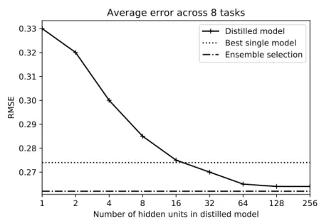
3.5 Model Distillation . . . 43
3.6 Filter Decomposition . . . 47
3.7 Summary . . . 52
4 RAPDARTS: Resource-Aware Progressive Differentiable Architecture Search 54 4.1 Introduction . . . 54
4.2 Related Work . . . 57
4.3 Method . . . 60
4.4 Experiments and Results . . . 66
5.1 Introduction . . . 73
5.2 Results . . . 77
5.3 Summary . . . 86
6 Distillation Strategies for Proximal Policy Optimization 88 6.1 Introduction . . . 88
6.2 Background and Related Work . . . 90
6.3 Formulation . . . 95 6.4 Implementation Details . . . 96 6.5 Results . . . 99 6.6 Summary . . . 102 7 Neuromorphic Engineering 103 7.1 Introduction . . . 103
7.2 Memristors Learn to Play . . . 104
7.3 Benchmarking Event-Driven Neuromorphic Architectures . . . 106
7.4 Event-Driven Neuromorphic Architectures . . . 108
7.5 Metrics . . . 109
7.6 Summary . . . 117
8 Conclusion 119 8.1 Future Work . . . 124
Introduction
How do you become an expert at something? Most likely it is through a combination of intense practice, instruction from a teacher, innate talent, and studying the work of other experts. Similarly, reinforcement learning (RL) is a branch of machine learning that attempts to create expert agents using various algorithmic approximations of the previous strategies. RL is distinguished from other machine learning methods by its use of a sequential decision-making agent that attempts to maximize the long-term collection of rewards within an environment. RL agents learn which actions, in which contexts, lead to the most rewards.
RL agents use a policy for action selection. In mammals, vision processing accounts for a significant portion of neural activity. Likewisedeep RL (DRL) policies often process visual or spatial inputs with the bulk of the policy’s computational expense attributable to the execution of convolutional neural networks (CNNs) or other types of deep neural networks (DNNs).
As an example of how computationally expensive DRL can be, consider DeepMind’s AlphaGo Zero (AGZ) reinforcement learning solution to the game of Go, which beat the world’s top Go player in 2016 [1]. AGZ used a large CNN for its policy.
Compu-tational cost was not clearly provided by DeepMind in the AGZ publication. However, Facebook Artificial Intelligence Research (FAIR) duplicated the AGZ work and provided a cost: 2,000 NVIDIA V100 GPUs running for 9 days [2]. Executing FAIR’s Go re-implementation code on Google Cloud would currently cost [3]:
2,000 GPUs× $2.48
GPU Hr×216 Hr ≈$1,071,360. (1.1)
The bulk of AGZ’s computational cost, and therefore financial cost, is its CNN-based policy which uses one input convolutional block followed by 19 residual blocks. The convolutional block has the following structure:
• 3×3 convolution with 256 channels and stride 1
• Batch normalization
• Rectified linear unit (ReLU)
The convolutional block output is input to a residual tower where each of the 19 residual blocks have the following structure:
• 3×3 convolution with 256 channels and stride 1
• Batch normalization
• ReLU
• 3×3 convolution with 256 channels and stride 1
• Batch normalization
• Skip-connection that adds the input
• ReLU
Go is partially-observable (because of a no-repeat rule in the game and because the current player is not indicated from the current board state) so the AGZ designers provide
the CNN with a history of recent board positions as well as an indicator for the current player. This is achieved by using 17 binary 19×19 (the game board size) channels as input to the policy. The first eight channels capture empty/occupy intersections of the current player’s stones for the last eight game states. The second eight channels capture the opponent’s stone intersections for the last eight game states. The 17th channel is set to all 1s, if it is black’s move, or all 0s, if it is white’s move.
Given AGZ’s network architecture and input tensor shape, approximately eight bil-lion multiply-accumulate operations (MACs) per forward-pass are required. The AGZ network is used for Monte-Carlo Tree Search (MCTS) during game play, using 1,600 game simulations to select each move. During each game simulation, the CNN is eval-uated once. Therefore, over 12 trillion MACs are required for the AGZ agent to pick a single move. This is why the AGZ network architecture is the primary contributor of the computational and financial cost for training and then deploying AGZ.
The computational intensity of DRL will only increase as tasks become more challeng-ing. Even now we are seeing DRL agents which receive as sensory input a mix of vision, audio, and text input [4, 5]. In addition to being required to process multimodal sensory inputs, agents must often perform in situations which require memory, because their in-stantaneous sensory inputs do not contain complete information about the state of their environment. Extending agents with complex memory capabilities further complicates design and increases processing cost.
The high computational expense of deep reinforcement learning will limit its application when constrained by power, memory, or latency. However, by extending deep neural network efficiency techniques to deep reinforcement learning, it is possible to both maintain agent performance and reduce the computational expense of the agent’s decision-making.
primitive operation, e.g. one of the following operations: convolution, pooling, attention, matrix-vector multiplication, recurrent operation, or nonlinearity operation. We refer to a DNN’s specific set of primitive operations and the connectivity between operations as the DNN’s architecture.
Similarly, we classify existing DNN optimizations into two categories: primitive op-timizations and architectural optimizations. Primitive optimizations are low-level, and they are concerned with obtaining the most benefit from the least amount of resources. This would be analogous to the development of a construction brick which can sup-port the most pressure and has the best insulation properties using the least amount of material. There are five primary primitive optimization strategies:
• Pruning: reduces the number of parameters, which, in turn, reduces the total number of MAC operations, amount of traffic required to transfer parameters, and storage requirements.
• Quantization: lowers the number of bits of precision representing neural network inputs, parameters, or activations, which lowers both memory requirements and silicon required for processing elements.
• Weight Sharing and Compression: forces parameters to share values, thus decreas-ing memory storage and traffic.
• Model Distillation: the training of a smaller network to mimic the behavior of larger network, reducing the number of parameters and lowering latency.
• Filter Decomposition: modifies convolutional filter designs such that the number of parameters and multiple-accumulate operations are reduced.
Architectural optimizations are concerned with the construction of DNNs, given spe-cific primitive operations with which to build from. Using another construction analogy,
the Passivhaus architectural standard achieves energy optimization through careful selec-tion of which construcselec-tion materials to use, HVAC flow, and the geographic orientaselec-tion of the building [6].
DNN architecture design has historically been a manual process, where various neu-ral network architecture and primitive combinations were iteratively hand-selected and tested on a dataset until something performed satisfactorily. Neural Architecture Search
(NAS) has recently started to take over hand-crafted architectural optimization.
NAS methods automate strategies for discovery of high performing neural architec-tures. A DRL approach was the first post-AlexNet NAS method with state-of-the-art performance on CIFAR-10 [7, 8]. The DRL approach was quickly followed by a high performance Evolutionary Strategy (ES) based method [9]. While both the DRL and ES methods discovered high performance architectures, their use came at the cost of thousands of GPU hours.
Gradient-based NAS (GBNAS) methods have the benefit of being directly optimized through gradient descent and consequently complete the search faster than other NAS methods [10]. The search process alternates between temporarily fixing one set of param-eters, i.e. assuming they are constant, and updating the other set of parameters. The GBNAS approaches provide no convergence guarantees, but they work well in practice.
Both primitive and architectural optimizations have been pursued extensively in su-pervised learning literature, but, to our knowledge, this dissertation represents the first comprehensive investigation into their application for efficient DRL.
There are close similarities between supervised learning and DRL, but analyzing the effect of optimizations on DRL should be considered explicitly. In both cases, image, audio, text, or other modalities, are input into a DNN for feature extraction. The resulting features are used for classification, in the context of supervised learning, action selection, in the context of DRL, or regression, which is used by both supervised learning
and DRL. The primary difference between supervised learning and DRL is the domain
of the inputs to the DNN.
In machine learning, the domain is the distribution over which the inputs to a func-tion are valid. In supervised learning, the training set is ideally drawn from the same distribution that the test set (or real-world examples) will be drawn from later. Extrap-olation occurs when inputs are drawn from a distribution that is different from which training has occurred.
DRL is more complex. In DRL, an agent may spend some time in one setting, e.g. a room. Observations from that setting will be used for DNN training. Eventually the agent may get to another setting, e.g. go outside. If the observational characteristics of the new setting are from a new distribution, then the DNN-based policy experiences domain shift, i.e. extrapolation occurs. Domain shift can cause collapse in agent performance.
The literature for DNN optimizations in supervised learning perform their evaluations on common benchmarks, e.g. CIFAR-10, CIFAR-100, ImageNet, in the case of CNNs. In that scenario, there is a known and fixed test set used by the community to compare results. The test set is essentially a previously agreed upon “holdout” subset of the training set. So research on primitive and architectural optimizations for supervised learning when using benchmarks for evaluation benefits from stable distributions.
On the other hand, domain shift is guaranteed to occur in non-trivial DRL environ-ments. A priori, it is unclear how primitive and architectural optimizations will react under the presence of domain shift in the DRL setting. For this reason it is worthwhile to specifically consider the impacts of DNN optimizations on the performance of DRL agents.
The optimizations discussed thus far are essentially concerned with the co-design of neural architectures and their constituent primitive operations to achieve efficient performance on observations from a domain of interest. Ultimately, however, a neural
architecture must be executed on a specific hardware platform. NVIDIA GPUs, and, increasingly, Google’s TPUs, are dominant for training DNNs, because they can effi-ciently perform high-precision tensor arithmetic over large training batches. However, for decision-making (i.e. inference), a CPU, GPU, FPGA, or custom accelerator may be preferable.
Taking hardware attributes and constraints into account is the next logical step when considering methods for efficient DRL. For example, there is no reason to prune individual convolutional filter parameters if hardware cannot take advantage of sparse convolution. And, for example, there is no reason to quantize numbers to single-bit precision, if the target processor’s ALU only supports a minimum of 8-bit arithmetic.
While this dissertation is primarily focused on DNN-based RL, we again point out that RL is a family of algorithms that learn behavior to maximize long-term accumulation of rewards. There is no requirement that RL algorithms use deep neural networks, indeed deep learning did not exist when the fundamental algorithms of RL were created [11, 12, 13]. However, before DNNs, the RL methods which used classical function approximation were not able to process high-dimensional observations well.
DNNs are a subset ofneuromorphic engineering which is concerned with biologically plausible models of intelligence. To put things in perspective, DNNs are an advancement over the McCulloch-Pitts neuron model which is essentially a dot-product and nonlinear-ity function [14]. The McCulloch-Pitts model was created in 1943. Since then, the field of neuroscience has advanced, and the field of computational neuroscience has appeared. These fields have created new mathematical models of neural processing. Many of the more biologically plausible neuromorphic computing models are based on spiking neuron models, which incorporate time and amplitude, unlike DNNs which only use amplitude [15].
18]. These are architectures that only perform computation when certain events occur, unlike common tensor processors which cannot benefit from sparse computations.
Thus far, the neuromorphic community has not found a training algorithm that trains spiking neuron models to perform as well as backpropagation trains DNNs. Partly this has to do with the fact that the deep learning community’s popular datasets are conducive to DNN processing, while spiking algorithms would benefit from event-driven datasets that are expensive to collect or generate. If and when the neuromorphic community is able to train event-driven models as well as backpropagation trains DNNs, then there will be opportunity to perform deep reinforcement learning at very low-power.
1.1
Dissertation Outline
• Chapter 2 introduces the basic mathematical concepts of Reinforcement Learning. Using Microsoft’s AirSim, we also provide a case-study of reinforcement learning’s application to drone flight control.
• Chapter 3 provides an overview of the central methods for primitive operation optimization: pruning, quantization, weight sharing and compression, model dis-tillation, and filter decomposition.
• Chapter 4 introduces a resource-aware neural architecture search technique. This method enables the discovery of DNNs which meet predefined resource constraints. As a use-case, we show how to discover CNN architectures requiring less than a specified number of parameters.
• Chapter 5 investigates the application of primitive operation optimizations to re-inforcement learning. In this chapter, we apply pruning, quantization, and com-pression to reinforcement learning policies and study how robust they are to the
optimizations.
• Chapter 6 develops a distillation algorithm for reinforcement learning which enables agents with relatively small CNN-based policies to achieve performance on par with agents using larger CNN-based policies.
• Chapter 7 considers neuromorphic hardware. In the first section, we analyze a recent memristive reinforcement learning accelerator. In the second section, we present an objective approach to the evaluation of neuromorphic hardware.
1.2
Permissions and Attributions
• The content of Chapter 2 is the result of a collaboration with Jieliang Luo, Peter Feghali, George Legrady, and C¸ etin Kaya Ko¸c. Part of the content previously appeared in Cyber-Physical Systems Security, C¸ . K. Ko¸c, editor, pages 191–217, Springer, 2018. It is reproduced here with permission from Springer.
• The content of Chapter 3 is the result of collaborations with Craig M. Vineyard, and C¸ etin Kaya Ko¸c. The content previously appeared in Cyber-Physical Systems Security, C¸ . K. Ko¸c, editor, pages 69–92, Springer, 2018. It is reproduced here with permission from Springer.
• The content of Chapter 4 is the result of collaborations with Craig M. Vineyard, and C¸ etin Kaya Ko¸c. It is currently in pre-publication.
• The content of Chapter 5 is the result of collaborations with Craig M. Vineyard, and C¸ etin Kaya Ko¸c. The content previously appeared at the International Joint Conference on Neural Networks, Rio de Janeiro, Brazil, July 8–13, 2018. It is reproduced here with permission from IEEE.
• The content of Chapter 6 is the result of collaborations with Craig M. Vineyard, and C¸ etin Kaya Ko¸c. The content is currently in review with IEEE Transactions on Neural Networks and Learning Systems. It is reproduced here with permission from IEEE.
• The content of Chapter 7 is the result of collaborations with Craig M. Vineyard, James B. Aimone, William Severa, and C¸ etin Kaya Ko¸c. Part of the content pre-viously appeared atInternational Conference on Neuromorphic Systems (ICONS), Knoxville, Tennessee, July 23–25, 2019. It is reproduced here with permission from the ACM. Part of the content previously appeared in Nature Electronics 2(3), 96, March, 2019. It is reproduced here with permission from Springer Nature.
Deep Reinforcement Learning
2.1
Introduction
Reinforcement learning (RL) is a family of control techniques that arose from a com-bination of applying psychological models of operant conditioning with mathematical techniques of dynamic programming [19]. In RL, there is an agent that uses a policy to decide actions, givenstate observations and rewards from an environment.
The agent may be something physical, like a robot, or it could be more virtual, like a program that chooses the advertisement to show a website visitor. Likewise, the environment may be physical or virtual. In general, actions can be discrete or continuous,
Agent Environment
state,
reward action
Figure 2.1: The deep reinforcement learning environment-agent cycle. An environ-ment provides state observations and rewards to an agent. State observations are input to a neural network-based policy which decides actions. An agent then makes an action with the goal of maneuvering into states with the highest rewards.
depending on the agent’s capability. Rewards can be continuous or discrete anddense or
sparse. An example of dense reward would be distance from the agent to a target at any given moment. An example of spare reward would be 0 at all time steps until some goal is reached and then 1 for only that time step. Finally, state observations represent the information an agent is able to detect from the environment. For example, a self-driving car may receive observations from only a CCD camera on it’s front bumper, or it could be surrounded by LIDAR, RADAR, CCD, and other sensors.
The agent’spolicy πmaps state observations to actions. The goal of all RL algorithms is to find an optimal policyπ∗that maximizes thereturn, which is defined as the expected sum of rewards over some sequence of state-action pairs. The environment provides state observations and rewards. After receiving a new observation, the policy chooses which action the agent should take. The policy must learn to make actions to maneuver the agent into states with high rewards. An illustration of the agent-environment interaction paradigm is shown in Fig. 2.1.
The optimal policy is then formally defined as:
π∗ = arg max π Eτ ∼p X t r(st, at) (2.1)
where therollout τ represents a sequence of states and actions, pis the trajectory distri-bution,ris thereward function mapping statessand actionsato rewards, and subscript t ranges across time steps in the rollout.
The basic methods of RL have been developed over the past several decades, but early RL algorithms did not work very well for high dimensional observations, e.g. images. Specifically, classical RL techniques using images for observations would require a table with each entry in the table corresponding to exactly one configuration of the image’s RGB values. For example, a 256×256 8-bit RGB image has 256×256×(28)3 ≈1×10¹²
Figure 2.2: In this chapter we train a drone to use its camera to perform path plan-ning. Training is performed via reinforcement learning, and the goal is to learn cam-era-to-action mappings that allow the drone to collect cubes.
possible unique values and would require a table with that many entries.
Function approximation can be used to map similar observations to similar actions. However, function approximation-based RL did not work well until 2013, when DeepMind developed new algorithms for using deep neural networks (DNNs) with RL. By doing so, in their seminal Atari-dominating RL work, agents learned to play many Atari video games at superhuman levels of performance [20]. Since then, there has been a regular stream of deep RL (DRL) algorithm improvements [21, 22, 23, 24]. The application space of DRL has naturally lagged behind theoretical results, and we expect to see further real-world results in the future. Following results, there will be increasing interest in hardware optimized for deep reinforcement learning.
In the remainder of this chapter, we introduce Markov Decision Processes, which are mathematical abstractions of many real-world decision making tasks. Then we introduce theVanilla Policy Gradient (VPG) method, which is a foundational reinforcement learn-ing algorithm. Finally, we apply VPG in the context of a physics-based simulator that enables experimentation with self-driving and flight applications (Fig. 2.2).
2.2
Markov Decision Processes
Markov Decision Processes (MDPs) are the mathematical models that reinforcement learning was developed to solve. MDPs have states in which an agent exists, and the
out-comes of actions depend only on the current state, not on past states and actions; in this sense MDPs arememoryless. The memoryless property is captured in the environment’s state-transition and reward function notation:
p(st+1|st, at, st−1, at−1, . . . , s0, a0) =p(st+1|st, at), r(st+1|st, at, st−1, at−1, . . . , s0, a0) =r(st+1|st, at).
(2.2)
The state-transition and reward functions in Eq. 2.2 specify that function outcomes depend only on the current state and action, and are independent of past states and actions.
A second defining feature of MDPs is that the state-transition and/or reward functions could be stochastic, which means their return values are drawn from some underlying probability distributions. In standard RL settings, these distributions must bestationary
which means the probabilities do not shift over time. Methods exist for using RL in nonstationary environments. Investigating such advanced methods is critical for using RL in safety-critical applications. For example, state-transition and reward distributions may shift from what was observed during training in the event of an anomalous situation, e.g. an emergency. In that case it could be disastrous were the agent to follow its policy decisions blindly. For that reason, consider the methods introduced in this chapter as an introduction to what is possible, but safety mechanisms should be put in place for real-world RL applications.
Within an MDP, agents may observe their current state and make actions that at-tempt to affect the future state. The agent’s objective is to maximize collection of rewards. An example 3-state MDP1 is given in Fig. 2.3. In this example, the initial state iss0, and the agent has two action options: a0 and a1. If the agent chooses actiona0 it is
1In the notation for this example, the subscripts for actions a denote “options”, versus the usual meaning, which is time in this chapter.
Figure 2.3: Example Markov Decision Process. There are three states and two ac-tions,a0 and a1. Unless otherwise indicated, the state transition probability is 1 and
reward is 0. Transition froms0 tos2 is the most interesting withr(s2|s0, a1) = 1 and p(s2|s0, a1) =.75.
guaranteed to stay in states0, denoted byp(s0|s0, a0) = 1. If the agent chooses actiona1, there is a 25% probability that it will transition to s1, denoted by p(s1|s0, a1) = .25, and a 75% probability it will transition tos2, denoted byp(s2|s0, a1) = .75. The environment returns reward of 0 for all state transitions except for s0 →s2, and in this case it returns r(s2|s0, a1) = 1.
In the context of Fig. 2.3 the agent should always select action a1, as it is the only action that leads to a non-zero reward. While we can see that is the solution, an RL agent must learn it.
2.3
Reinforcement Learning Approaches
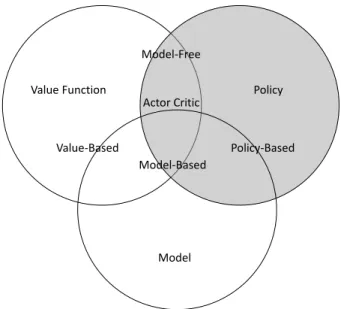
As illustrated in Fig. 2.4, the approaches for finding the optimal policy π∗ in Eq. 2.1 can be separated into three families of methods: value-based methods, policy-based methods, and model-based methods. Value-based methods, e.g. Q-Learning, are closer to RL’s historical roots in dynamic programming. They use the learned value of states and actions to find a policy that will transfer the agent into states with more value [12, 25, 26]. Policy-based methods directly learn to optimize an action-making policy via maximizing a reward function [24]. Model-based approaches require the agent have a representation of the environment which provides a prediction of the reward the environment will yield when a given action is taken [27]. This model of the environment enables learning the
Value Function Policy Model Value-Based Model-Free Actor Critic Model-Based Policy-Based
Figure 2.4: Reinforcement learning taxonomy of approaches. Value-based methods learn the long-term results of states or state-action pairs. Policy-based methods learn to directly optimize a policy. Model-based methods leverage given or learned me-chanics of the environment. This introductory chapter is focused on a policy-based method.
optimal policy by providing a prediction of how the environment will behave so the best actions to take may be identified. It is also possible to mix value-based, policy-based, and model-based methods into hybrid RL algorithms [28, 29].
Because they serve as the basis for most deep RL approaches, we focus on policy-based methods in this chapter, highlighted in gray in the figure, and described in more detail next.
2.4
Vanilla Policy Gradient
In the context of reinforcement learning, our first-order objective was defined in Eq. 2.1 as the sum of rewards, but here we will refine it. As stated in Section 2.2, MDPs often have stochastic state transition and reward functions; for that reason the
objective J(θ) of the agent is actually to maximize the expected sum of rewards under the trajectory distribution (defined in Eq. 2.8 below). This is achieved by discovering
optimal policy (i.e. deep neural network) parameters θ? that maximize the objective function J(θ): θ? = arg max θ E τ∼pθ T−1 X t=0 r(st, at) = arg max θ J(θ), (2.3)
where τ is the trajectory of state-action pairs (s0, a0, s1, a1, . . . , sT, aT) and pθ is the trajectory distribution which is conditioned on the policy parameters.
The Vanilla Policy Gradient method uses gradient ascent to adjust the policy pa-rameters in a direction that increases J(θ) [13]. For notation convenience let r(τ) =
PT−1
t=0 r(st, at), and by the definition of expectation, the objective can be written as:
J(θ) = Eτ∼pθr(τ) = X
τ
pθ(τ)r(τ), (2.4)
where pθ(τ) is the probability of a specific trajectory, and there may be a finite or countably infinite different number of trajectories τ. Taking the gradient of J(θ) with respect to θ then gives:
∇θJ(θ) = ∇θ X τ pθ(τ)r(τ) = X τ ∇θpθ(τ)r(τ). (2.5)
For reasons that will become clear, we recall the following identity:
∇θpθ(τ) = pθ(τ)
∇θpθ(τ) pθ(τ)
=pθ(τ)∇θlog(pθ(τ)), (2.6)
allowing us to rewrite Eq. 2.5 as:
∇θJ(θ) = X τ pθ(τ)∇θlog(pθ(τ))r(τ), =Eτ∼pθ∇θlog(pθ(τ))r(τ). (2.7)
(i.e. experienced) trajectory τ has a probability that can be explicitly calculated only if the underlying state-transition function is known:
pθ(τ) =p(s0) T−1
Y
t=0
πθ(at|st)p(st+1|st, at), (2.8)
where p(s0) is the probability of starting the trajectory in state s0 and is independent of θ, and πθ(at|st) is the probability of the selected action given the state observation st. To better understand the notation πθ(at|st), note that the policy is stochastic. In other words, when the policy is given a state observation st, the output of πθ(st) is a vector of probabilities derived from the sof tmax function2. In the discrete action-space environments considered here, there is one output probability per possible action. A random action is then drawn from the given probability distribution, and the probability of the selected action is denotedπθ(at|st).
In real-world problems, the environment’s state transition function p(st+1|st, at) is not known, so pθ(τ) would be impossible to calculate. However:
logpθ(τ) = log p(s0) T−1 Y t=0 πθ(at|st)p(st+1|st, at) = logp(s0) + T−1 X t=0 logπθ(at|st) + logp(st+1|st, at), (2.9)
and replacing logpθ(τ) in Eq. 2.7 with its expanded form gives:
∇θJ(θ) = Eτ∼pθ∇θ h logp(s0) + T−1 X t=0 logπθ(at|st) + logp(st+1|st, at) i r(τ), =Eτ∼pθ T−1 X t=0 ∇θlogπθ(at|st)r(τ). (2.10) 2sof tmax(x i|x) := exp(xi) P|x| j=1exp(xj)
In this form, we are able to approximate the gradient. Recall that πθ is a neural network (or some other differentiable function), so the gradient of its log may be calculated explicitly given each at and st over the trajectory. Also, we know the sum of rewards r(τ) for each trajectory. Finally, the outer expectation is approximated by performing N episodes, i.e. experiencing multiple trajectories, and then averaging the sums giving:
∇θJ(θ)≈ 1 N N X n=1 T−1 X t=0 ∇θlogπθ(an,t|sn,t)r(τn). (2.11)
After having obtained an approximation of the objective’s gradient, we may use it to update the neural network parameters with standard stochastic gradient ascent:
θ =θ+α∇θJ(θ), (2.12)
whereα is the learning rate and whose appropriate value must be experimentally found. The Vanilla Policy Gradient method works surprisingly well for a broad range of problems, and there are many improvements that have been made to it to increase its performance. Understanding the method presented here is a good foundation for approaching current literature. The derivation of the Vanilla Policy Gradient method as presented above is credited to [30].
2.4.1
Vanilla Policy Gradient Method in AirSim
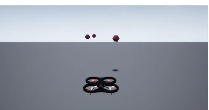
We now apply the Vanilla Policy Gradient method to a cube collection task, illustrated in Fig. 2.5. We have extended Microsoft’s AirSim simulator to support teaching a drone how to autonomously navigate a sequence of visual waypoints. This is captured by randomly distributing cubes in front of a drone at the start of each episode. The drone receives a reward for each cube it reaches. In this environment, the drone has a discrete
Figure 2.5: Example of our custom AirSim environment. After the environment is reset, cubes are placed randomly in front of the drone. The drone has a camera that provides input to a reinforcement learning agent. The agent contains a CNN-based policy and learns how to use the camera input to infer control decisions for collection of cubes.
action space of forward, left, and right. The observation space is continuous and is derived from a camera mounted on the drone. The source code for these experiments is available at https://github.com/RodgerLuo/CPS-Book-Chapter.
A convolutional neural network is used to represent the policy. We will refine the objective (from Eq. 2.3) of finding network parameters that maximize the expected sum of rewards across all time steps in the episode:
θ? = arg max θ E τ∼pθ T−1 X t=0 r(st, at).
In the cube collection task, a reward of 1 is provided by the environment each time step a cube is collected by the drone, and 0 reward when no cube is collected, so the objective is to collect as many cubes as possible in each episode (i.e. during time stept = 0...T−1, where T −1 is the step when the last cube is collected or the drone has gone out of
bounds). In the context of Vanilla Policy Gradient, this objective was discovered by taking its gradient (from Eq. 2.11):
∇θJ(θ)≈ 1 N N X n=1 T−1 X t=0 ∇θlogπθ(an,t|sn,t)r(τn),
and then updating the neural network parameters based on the gradient. Recall that πθ is the neural network, and, in the drone collection task, πθ(an,t|sn,t) is the output probability3 of going left, right, or forward, given input pixels from the drone’s camera.
One weakness of Eq. 2.11 for our context is that the rewards are sparse, because there are only three cubes total to collect in each trajectory. If the episode return r(τn) is used directly as the reinforcing signal thenentire trajectory probabilities are increased or are unchanged. This results in high variance in performance between each episode. An approach to get faster results in the cube collection task is to “smooth” the attribution of rewards from later stages to earlier stages by applying adiscounted return to the gradient at each time step. The discounted return is defined as:
gt=rt+1+γrt+2+γ2rt+3+· · ·+γT−t−1rT−1 = T−1
X
k=t
γk−trk, (2.13)
whereγ ∈[0,1] is the discount rate. The resultinggvector of Eq. 2.13 is also normalized4 in the cube collection task. Using g we update Eq. 2.11 to give:
∇θJ(θ)≈
T−1
X
t=0
∇θlogπθ(at|st)gt, (2.14)
where we are only collecting a single trajectory between applications of gradient ascent.
3Softmax of the network’s logits.
4Normalization is defined asg←(g−µ(g))/σ(g), where scalar operations are applied element-wise to the vector.
There are much better approaches than using the discounted return, and our source code example is parameterized to allow experimentation with other reward function alterna-tives.
Algorithm 1: Vanilla Policy Gradient algorithm in the context of the AirSim cube collection task.
Input: Old policy parameters θ, learning rate α, tuple of (observations s, actions a, rewards r) from last cube collection episode
Output: Updated policy θ
1 Apply Eq. 2.13 to obtain discounted rewards g from a 2 Normalizeg
3 Set sum of grads = 0 4 for t = 0. . . T −1 do
5 sum of grads=sum of grads+gt∇θlogπθ(at|st) 6 end
7 θ =θ+αsum of grads 8 return θ
We summarize the use of the Vanilla Policy Gradient method in the context of our AirSim cube collection task in Algorithm 1. This algorithm is implemented in the pro-vided source code and will train a drone to collect cubes based on visual observations.
2.5
Summary
In this chapter we introduced the Markov Decision Process, which is the sequential decision making mathematical model that reinforcement learning solves. We also intro-duced the basic families of reinforcement learning: policy-based, value function-based, and model-based. We then provided a derivation of the Vanilla Policy Gradient method, which is the foundational policy-based algorithm. The VPG method was then used to train a drone to collect cubes in Microsoft AirSim.
Mathematical Optimizations for
Deep Learning
3.1
Introduction
Modern DNN architectures require billions of floating-point multiplications and ad-ditions (MACs) for inference of a single input. Without careful design, this results in high power consumption and high latency. Fossil-fuel powered vehicles, for example, can support high energy demands, but efficient, battery powered systems cannot. Addition-ally, modern large DNNs have high latency, but low latency is required for real-time autonomous applications. This chapter provides a unified view of the leading methods for mathematically-optimized deep learning inference. The methods introduced in this chapter will be applied to deep RL algorithms and applications in following chapters.
To motivate the need for optimizations, it is helpful to consider first-order power and silicon area requirements for DNN inference. Table 3.1 provides a list of energy and die area required for various operator and operand sizes. Observe that a single 32-bit floating-point multiplication (denoted “32b FP Mult”) requires 20 times more power and
Operation Energy (pJ) Area (um) 8b Add 0.03 36 16b Add 0.05 67 32b Add 0.1 137 16b FP Add 0.4 1360 32 FP Add 0.9 4184 8b Mult 0.2 282 32b Mult 3.1 3495 16b FP Mult 1.1 1640 32b FP Mult 3.7 7700
32b SRAM Read 5 N/A
32b DRAM Read 640 N/A
Table 3.1: Energy and die area costs for various operations (45nm) [31]. Quantized operators and operands are preferred for low-power and low-resource applications. FP stands for floating-point.
12 times more area than 8-bit integer multiplication (“8b Mult”). Also observe that the power cost of a 32-bit DRAM read is more than 100 times the cost of floating-point multiplication. For this reason, efficient DNN implementations should prioritize the minimization of off-chip DRAM access first, followed by reducing operand and operator sizes. Naturally these two approaches complement one another.
DNN optimizations are useful only during the inference operation. Currently, training a DNN to reach state of the art performance requires the backpropagation algorithm, which uses gradient descent to make many small adjustments to the neural network parameters. These small adjustments must be calculated and stored using full-precision accumulation. Therefore the optimizations discussed in this chapter are not primarily aimed at making training more efficient, but they are intended to make inference more efficient.
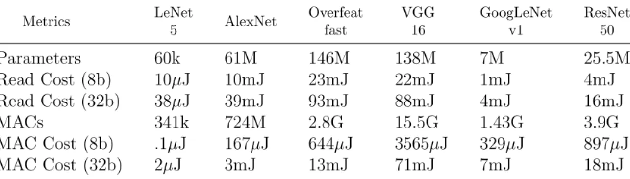
To further emphasize the need for inference efficiency, consider the number of opera-tions required to evaluate various modern DNNs, given in Table 3.2. This table provides a first-order estimate for MAC and memory costs for popular DNN architectures. Power
estimates assume 32-bit floating-point arithmetic and are derived from Table 3.1. MAC costs capture the power requirement for each network to perform the necessary operations for providing a single inference. The memory cost is best-case and assumes parameters are read from DRAM only once per inference; actual memory costs will be higher if inter-mediate results must be transferred back to DRAM during inference of the network. In Table 3.2 note that even though the number of MACs are much greater than the number of parameters, the high DRAM read cost results in the power consumed between the two to be roughly equivalent. Metrics LeNet 5 AlexNet Overfeat fast VGG 16 GoogLeNet v1 ResNet 50 Parameters 60k 61M 146M 138M 7M 25.5M Read Cost (8b) 10µJ 10mJ 23mJ 22mJ 1mJ 4mJ Read Cost (32b) 38µJ 39mJ 93mJ 88mJ 4mJ 16mJ MACs 341k 724M 2.8G 15.5G 1.43G 3.9G MAC Cost (8b) .1µJ 167µJ 644µJ 3565µJ 329µJ 897µJ MAC Cost (32b) 2µJ 3mJ 13mJ 71mJ 7mJ 18mJ
Table 3.2: Number and cost of parameters and MACs for popular deep neural network architectures. Cost estimates are based on Table 3.1 and from archi-tecture statistics provided in [32]. Note that memory costs are typically higher than MAC costs.
The process of DNN training may be thought of as an exploration over a param-eter space to find values which will solve an inference task. As will be expanded on, the parameters found using standard training methods result in DNNs which are over-parameterized, which means they have redundancy. When the DNN performs satisfacto-rily during cross-validation, backpropagation is no longer needed, and optimizations may be applied to decrease parameter redundancy. The goal of mathematical optimizations for deep learning is to find the most compact network which performs satisfactorily at
its assigned real-world inference tasks.
DNN architectures are composed of various layer types: convolutional, fully-connected, dropout, pooling, and others. Each layer type was developed to solve a particular weak-ness and each classification problem is best solved by a different architecture, or combi-nation of layers. Convolutional and fully-connected layers represent the greatest compu-tational expense in DNN inference, and optimizing these layer types is the focus of this chapter. Both convolutional and fully-connected layers require repeated multiplication and addition, but they typically use different algorithmic steps. Adapting notation of [33], we represent an L-layer DNN ashI,W,Oi, where:
• Il ∈ Rcin×x×y and Wl ∈ Rcin×w×h×cout are layer l’s input tensors and parameter tensors respectively. cin represents the number ofinput channels andcoutrepresents the number of output channels1. x and y are the width and height of each input channel, and w and h are the width and height of each filter.
• Ol ∈ {∗,·,other} specifies whether the layer’s operation type is convolution (∗), fully-connected (·), or some other less computationally expensive type.
Convolutional layers convolve aRcin×w×h×cout parameter filter tensor with a
Rcin×x×y
input tensor, where (w,x) and (h,y) represent the widths and heights of the two respective tensors and may be different sizes, and cin and cout represent the number of input and output channels. In particular the (w, h) for parameter filters are often smaller than the (x, y) for inputs. c is the number of channels in the given layer; this value is equal for both the parameter filter tensor and input tensor. As illustrated in Figure 3.1 (top), each step in the convolution requires a sum of products between elements of the parameter filter and elements of the receptive field of the input filter.
} } }
} }
Figure 3.1: Convolutional layers convolve a parameter filter with an input. Filters are usually 5×5, 3×3, or 1×1. Each step of the convolution involves multiplying and accumulating elements of the parameter filter with areceptive field of the input. The top illustration represents the basic convolution operation (∗). The lower illustration representscout,cin-channel filters which are convolved with acin-channel input tensor,
which results in ancout-channel output tensor.
Figure 3.2: Fully-connected layers flatten the input tensor into a vector and multiply by a parameter matrix with the same number of columns as the vector and as many rows as desired.
Note that what is shown in Figure 3.1 (top) only depicts convolution of a single channel. If there are multiple channels, then the summation is also over all channels. Figure 3.1 (bottom) shows a higher-level view, where eachcin-channel parameter filter is convolved with thecin-channel input tensor. When multiple channels are included in the convolution, each output of the convolution becomes the triple-sum across the channels. The number of parameter filters in a layer equals the number of channels in the output tensor: if there arecout parameter filters, there will becout channels in the output tensor. Computation for fully-connected layers requires a single matrix-vector product. The input tensor Il ∈ Rcin×x×y is flattened to a vector ∈ Rcin·x·y. The parameter tensor is denotedW ∈Rw×h, wherew=cin·x·y(from the input tensor dimensions) andhis equal
to the number of desired output units from the fully-connected layer. An illustration of a fully-connected layer is given in Fig. 3.2.
After a parameter filter W is convolved with an input I in a convolutional layer, or the matrix-vector product between parameters and layer inputs is produced for a fully-connected layer, the resulting matrix of vector entries are typically passed through a nonlinearity function σ : R → R. A commonly used nonlinearity is the rectified-linear unit (ReLU), which is defined as:
σReLU(x) = x if x≥0, 0 else. (3.1)
But more extreme nonlinearities exist, such as the binarized activation function which outputs only two values, −1 and 1:
σb(x) = 1 if x≥0, −1 else. (3.2)
The choice of nonlinearity function influences the performance and computational cost of inference. Specifically, using the binarized activation function can lead to the elimination of floating-point and fixed-point arithmetic during inference, as detailed in Subsection 3.3.2.
Both convolutional and fully-connected layers require many memory access and MAC operations, but a variety of numerical optimizations may be applied to DNN inference. Some optimizations reduce power and some optimizations reduce both power and latency. Furthermore, it is possible to optimize a DNN and maintain classification accuracy, but there also exist extreme optimization methods which result in unavoidable accuracy loss.
Depending on the application, decreased accuracy may be worth the reduction in power and latency.
The remainder of this chapter provides an introduction to the common approaches of DNN mathematical optimization: pruning, quantization, parameter sharing and com-pression, model distillation, and filter decomposition.
3.2
Pruning
Pruning applies to fully-connected and convolutional layers and eliminates each layer’s smallest parameters, which has the consequence of reducing the number of MAC oper-ations, the amount of traffic required to transfer parameters, and storage requirements. The typical procedure is to train the network until the desired accuracy is reached and then to prune the smallest pth-percentile of parameters by setting them to zero. Pruning is followed by fine-tuning the remaining parameters, which can be accomplished using the same dataset as used during initial training.
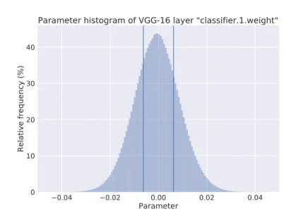
In [35], the authors report 9× and 13× reduction in parameters for AlexNet and VGG-16 with no impact on test accuracy. A histogram of the normalized frequency of parameters is given in Fig. 3.3, where the smallest 50th-percentile is delineated with two vertical lines. In practice, one would pick the percentile threshold for each layer heuristically, that is, the percentile threshold would be a hyperparameter for each layer. This process is represented in Algorithm 2.
After pruning, the resulting DNN will be sparse, with many parameters set to zero. Standard architectures, like GPUs, are currently not designed to take advantage of spar-sity and will perform multiplication regardless if one of the operands is zero. In order to benefit from pruning, the architecture must be designed in such a way as to take advan-tage of sparsity. This will add edge cases to standard logic design. For example, consider
0.04 0.02 0.00 0.02 0.04 Parameter 0 10 20 30 40 Relative frequency (%)
Parameter histogram of VGG-16 layer "classifier.1.weight"
Figure 3.3: Histogram of parameters of the first fully-connected layer in VGG-16. The name “classifier.1.parameter” corresponds to the VGG-16 implementation found in torchvision [34]. The two vertical lines correspond to thresholds of values smaller than the 50th-percentile. These values may be pruned (permanently set to zero) and the remaining values fine-tuned with no loss in accuracy [35]. The same procedure may be applied to all other layers in the network.
a product summation tree, which can parallelize MAC operations. Even if the tree is designed to ignore products with a zero operand, it must still take into account that the zero product must be passed to the next tree level at the appropriate time. Recently, architectures for handling sparse dataflows have been developed. One such architecture reduces the amount of “wasted” logic required for ignoring zero-products by only passing non-zero products to processing elements downstream [36].
3.3
Quantization
Before 2015, most DNNs were trained using 32-bit floating-point arithmetic. In this section we summarize approaches for using reduced precision, or quantized, arithmetic for DNN inference. Quantization reduces the amount of parameter data that must be transferred from DRAM to processing elements. Additionally, quantized arithmetic is less
Algorithm 2:Pruning
Require: L-layer DNN hI,W,O,Pi, whereIl and Wl are layer l’s input tensors and parameter tensors respectively, andOl specifies whether the layer’s type is
convolutional, fully-connected, or some other type, and P is the pruning percentile for each layer.
Ensure: Pruned and fine-tuned network parameters W.
1. Initial training:
Perform standard training of DNN until satisfactory performance is achieved.
2. Pruning:
For each layerl in hI,W,O,Pi, eliminate parameters in Wl which are less than layer l’s pth percentile, where p=Pl.
3. Fine-tuning:
Perform standard re-training of remaining parametersW, until maximum performance is achieved.
expensive in terms of power and silicon area than full-precision arithmetic. Quantization may be applied to parameters, activations, or both parameters and activations. We emphasize that quantization techniques using <16-bits currently only provide efficiency benefits during inference, because backpropagation requires accumulation of small values, and therefore ≥16-bits.
It appears that 8-bit or 16-bit quantization is adequate for most DNN inference tasks. For example, Google’s DNN accelerator, the Tensor Processing Unit (TPU), exclusively uses 8-bit or 16-bit integer arithmetic [37]. The TPU (and the successor TPUv2) has become a critical component of Google’s computing ecosystem. Additionally, NVIDIA’s Pascal architecture was designed to support 16-bit floating-point and 8-bit integer arith-metic.
In this section we focus on extreme quantization methods which binarize parameters and activations. Binarization usually has a large negative impact on performance, but we present techniques in Subsections 3.3.1 and 3.3.2 which reduce the impact.
to both convolutional and fully-connected layers. In a convolutional layer, a c-channel parameter filter W ∈ Rc×w×h is convolved with an input I ∈
Rc×w×h. Convolution is
performed by W ∗ I. At a specific receptive field, the core operation may be interpreted as the inner-products between vectors. In this section, we sometimes use the notation
W>I to denote the convolution of a filter with a specific receptive field. Simultaneously, the W>I notation captures the partial calculation of a fully-connected layer.
3.3.1
Binary parameters
In 2015, BinaryConnect [38] was an early DNN quantization method, and exemplifies the field’s approach to quantization. During inference, BinaryConnect quantizes full-precision DNN parameters W to{−1,1}, using the sign function:
w(b) = +1 if w≥0, −1 else. (3.3)
Equation 3.3 discards real-valued information, but, in doing so, it also eliminates the need for floating-point multiplication during inference. Instead, signed floating-point addition may be used for unit activation input calculations. During backpropagation, the error caused by quantization is used to update the real-valued Ws. After training is complete, full-precision parameters and arithmetic are no longer required and may thereafter be discarded. From a hardware perspective, memory overhead is 32×less when using BinaryConnect-derived parameters. However, this technique has an accuracy cost. When using the AlexNet DNN architecture, BinaryConnect achieves 61% top-5 accuracy on ImageNet, compared to 80.2% accuracy when using AlexNet with 32-bit full-precision accuracy [33].
bias terms fromW, where normally it is included in that tensor for notation convenience. The reason here is that the bias is always added, even with full-precision arithmetic, so there is no benefit to quantize it. Also note theclip function in Algorithm 3 limits the full-precision parameters to between [−1,1].
Algorithm 3:BinaryConnect [38]
Require: Inputs I, targetsy, previous full-precision parameters W, biases b, learning rate η, and objective function J.
Ensure: Updated {−1,1}-valued parameters W(b) and real-valued bias b.
1. Forward propagation: A0 =I
forl = 1 to L
for kth filter in lth layer
Wlk(b) ← binarize(Wlk) using Equation 3.3
Alk ← W (b)
l ∗ A(l−1)k+blk
2. Backward propagation:
Initialize output layer’s activation gradient ∂A∂J
L using y, AL, andJ
forl =Lto 2
for kth filter in lth layer Compute ∂A∂J (l−1)k knowing ∂J ∂Alk and W (b) lk 3. Update parameters: Compute ∂∂JW lk and ∂J ∂blk, knowing ∂J ∂Alk and A(l−1)k W ← clip(W −η∂∂JW) b←b−η∂J∂b
Not made explicit in Algorithm 3 is how the gradient signal passes through the bina-rization function given in Equation 3.3. This is required for calculation of∂J/∂Wlk(b). We cannot merely take the derivative of the binarization function, because it is 0 everywhere except at W = 0, where the function is discontinuous. To handle this, the authors used a variant of the Straight-Through Estimator (STE) during backpropagation [39]. The
modified STE is defined as: STE(x) = 0 if x <−1, 1 if −1≤x≤1, 0 if x >1. (3.4)
During backpropagation, the derivative of the parameter binarization function (Eq. 3.3) is calculated with respect to each full-precision parameter: dW
(b)
lk
dWlk. Because the
pa-rameter binarization function is discontinuous, its derivative must be estimated, which is achieved by replacing it with theSTEevaluated at the full-precision parameter. Multi-plying by the STE during backpropagation has the effect of canceling the gradient when the full-precision parameter’s magnitude is too large.
To summarize BinaryConnect, we take the sign of the real-valued parameters dur-ing inference. Durdur-ing backpropagation, the errors caused by binarization may be very small (with significant changes accumulating over many inputs) and we track those small changes in precision versions of the parameters. After training is complete, the full-precision parameters may be discarded, only keeping their sign information.
XNOR-Net [33] introduced a method which is almost identical to BinaryConnect, but it performs binarization in a way which achieves higher accuracy. As with BinaryConnect, parameters are binarized during inference, but then they are also scaled by a factor which attempts to compensate for the binarization. Specifically, XNOR-Net introduced the following approximation for the inner-product2:
W>I ≈αW(b)>I
, (3.5)
where W(b) is the binarized version of W using Equation 3.3. This notation is slightly different than that used in Algorithm 3, where we are able to binarize the entireW tensor at once. But with XNOR-Net, each filter in each convolutional layer requires a separate α. To keep the notation simple, separate filters are not denoted.
To find the optimal scaling factorα, we solve the following optimization problem:
J(α) =W −αW(b) 2 , α∗ = arg min α J(α). (3.6)
That is, we are seeking an α which minimizes the distance between W and αW(b). For intuition, consider a scalar w and its binarized version w(b); in this case α = w/w(b) perfectly minimizes the distance between w and w(b). Expanding the norm in Equation 3.6 gives:
J(α) = α2W(b)>W(b)−2αW>W(b)+W>W. (3.7)
We now take the derivative of J(α) with respect to α, set it to zero, and solve for α:
dJ(α)
dα = 2αW
(b)>W(b)−2W>W(b). (3.8)
Let n = W(b)>W(b), which is also equal to the number of parameters in the binarized filter. Substituting n into Equation 3.8, setting it to zero, and solving for α gives α∗:
α∗ = W (b)>W(b) n = W(b)>sign(W) n = P |W| n . (3.9)
New α∗s must be calculated every time W changes, i.e. each time backpropagation is used to update the parameters, but, after the training is completed, α∗ may be saved for use during inference.
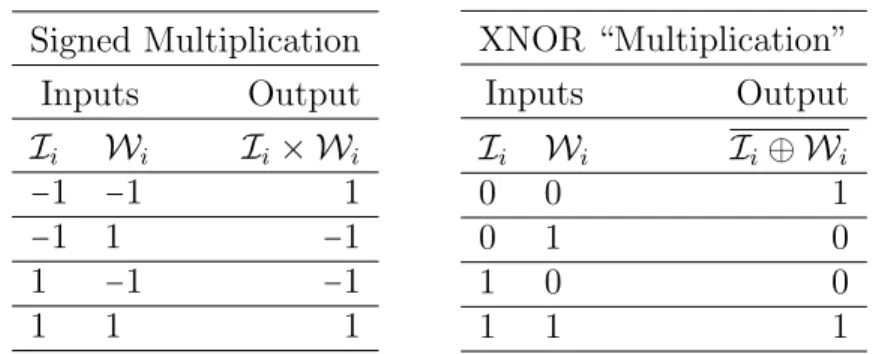
Signed Multiplication Inputs Output Ii Wi Ii× Wi −1 −1 1 −1 1 −1 1 −1 −1 1 1 1 XNOR “Multiplication” Inputs Output Ii Wi Ii⊕ Wi 0 0 1 0 1 0 1 0 0 1 1 1
Table 3.3: The XNOR operation captures the behavior of signed multiplication.
Using the parameter binarization methods above, we may eliminate most multipli-cations from inference3, and instead we only need signed addition. If we assume 32-bit multiplication and addition, this results in 32× power reduction for parameter transfer from DRAM and ∼ 3× power reduction for arithmetic. When using the AlexNet DNN architecture, XNOR-Net (binary parameters, full-precision activations) achieves 79.4% top-5 accuracy on ImageNet, compared to 80.2% accuracy when using AlexNet with 32-bit full-precision accuracy [33]. We next consider operator optimizations which become available when both parameters and inputs are binarized.
3.3.2
Binary parameters and Activations
If parameters and activations are binarized, then we are able to eliminate almost all floating-point (and fixed-point) calculations, resulting in extreme energy savings. Specif-ically, when parameters and inputs are binarized, the XNOR operation4 may be used to calculate inner-products during inference [40]. The XNOR logic truth table is given on the right in Table 3.3. The left-hand side provides the truth table for signed multiplica-tion between scalar values Ii ∈ I and Wi ∈ W. Note that by mapping −1 to 0, the two tables give identical output.
3Multiplication byαis still necessary when using the parameter binarization technique in XNOR-Net.
XNOR logic is simple and efficient to implement in hardware and may be used as the multiplication operator for the calculation of inner-products during inference. To use the XNOR “product” between I and W for the input into a unit’s nonlinearity function, we first map all −1s to 0s, then calculate the XNOR values for both vectors. The Hamming parameter5 (HW) of the XNOR vector result is then compared to #bits/2, where #bits is the size of W and I. If the Hamming parameter is greater than or equal to #bits/2 then output 1, otherwise output 0. Note that after the initial mapping of −1 to 0, we no longer need to map back to −1 during the remainder of the inference procedure.
BinaryNet [40] operates similarly to BinaryConnect, with the addition that activa-tions are also binarized. When using BinaryNet, the activation inputs are summed, as with BinaryConnect, and then the resulting sum is converted to [−1,1] using the sign function. This optimization eliminates all full-precision calculations and replaces them with signed integer calculations. As with BinaryConnect, BinaryNet requires full-precision gradient updates during training, and during backpropagation theSTEfunction (Eq. 3.4) is used for both the activation and parameters. BinaryNet achieves 50.42% top-5 accuracy on AlexNet, compared to 80.2% accuracy when using the same DNN topology and 32-bit full-precision accuracy [33].
XNOR-Net also has a version which binarizes both parameters and activations. Simi-lar to XNOR-Net’s parameter-only binarization presented above, there is a scaling factor αwhich may (optionally) be used to reduce the error between full-precision and binarized dot products: J(α) = I>W −αI(b)>W(b) 2 , α∗ = arg min α J(α). (3.10)
This is solved in the same manner as Equation 3.6, giving: α∗ = P |I(b)>W(b)| n = P |I||W| n . (3.11)
Note that a separate scaling factor α∗ must be solved for each receptive field and pa-rameter filter combination both during training and when using the neural network after training. This high computational overhead limits the use of vanilla XNOR-Net. Fortu-nately, in practice, the authors of BinaryNet found that the scaling factor for binarized parameters was much more important than the scaling factor for binarized inputs, and may therefore be ignored. We summarize the parameter-scaled version of XNOR-Net with the following algorithm:
Algorithm 4:(parameter-scaled) XNOR-Net [40]
Require: Inputs I, targetsy, previous full-precision parameters W, biases b, learning rate η, and objective function J.
Ensure: Updated {−1,1}-valued parameters W(b), parameter scaling factors α, and real-valued biasb.
1. Forward propagation: A0 =binarize(I0)
forl = 1 to L
for kth filter in lth layer αlk= n1||Wlk||`1
Wlk(b) ← binarize(Wlk) using Equation 3.3
A(lkb) ←binarize (αlkW (b) lk )∗ A (b) (l−1)k+blk using Equation 3.3 2. Backward propagation:
Initialize output layer’s activation gradient ∂J
∂AL using y, AL, andJ
forl =Lto 2
for kth filter in lth layer Compute ∂J ∂A((bl−)1)k knowing ∂J ∂A(lkb) and Wlk 3. Update parameters: Compute ∂J ∂Wlk(b) and ∂J ∂blk, knowing ∂J ∂A(lkb) and A(l−1)k W ← clip(W −η∂W∂J(b)) b←b−η∂J∂b
Similar to the calculation of∂J/∂Wlk(b)in Algorithm 3, both partial-derivatives∂J/∂Wlk(b)
and∂J/∂A(lkb)in Algorithm 4 are substituted with theSTEfunction in Equation 3.4, where the inputs toSTE are the real-valued parameter and activation respectively.
XNOR-Net using binarized inputs and parameters achieves 69.2% accuracy on AlexNet, compared to BinaryNet’s 50.42%, and full-precision accuracy of 80.2%. The XNOR-Net and BinaryNet papers introduce other training tips for improved performance. The aggregate contributions of the performance techniques introduced in XNOR-Net likely account for its significant gain over BinaryNet.
3.4
Parameter Sharing and Compression
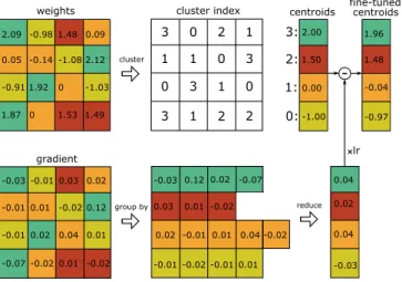
Top-performing neural networks use millions of parameters which are typically trans-ferred from DRAM to processing elements for inference (see Table 3.2). When these parameters are transferred, DRAM energy cost can surpass arithmetic cost for perform-ing a sperform-ingle inference. Parameter sharperform-ing clusters parameters into shared values and is applied after the network has reached peak performance. Once parameters have been clustered, compression may be used to transmit cluster indices instead of full-precision values. Parameter sharing coupled with data transfer compression is a method to retain the high performance typically provided by large full-precision neural networks, while simultaneously reducing the amount of data sent over DRAM [35].
3.4.1
Parameter Sharing
To apply parameter sharing, first, the DNN is trained to maximum performance using standard training methods. After training, each layer’s parameters are grouped into clusters, where the number of parameters in a layer is much greater than the number of clusters. After assigning parameters to clusters, the network goes through a retraining
![Table 3.1: Energy and die area costs for various operations (45nm) [31]. Quantized operators and operands are preferred for low-power and low-resource applications](https://thumb-us.123doks.com/thumbv2/123dok_us/9903071.2483649/36.918.267.683.161.424/energy-operations-quantized-operators-operands-preferred-resource-applications.webp)