(will be inserted by the editor)
Optimizing Different Loss Functions in Multilabel
Classifications
Jorge D´ıez · Oscar Luaces · Juan Jos´e del Coz · Antonio Bahamonde
Received: date / Accepted: date
Abstract Multilabel classification (ML) aims to assign a set of labels to an instance. This generalization of multiclass classification yields to the redefinition of loss functions and the learning tasks become harder. The objective of this paper is to gain insights into the rela-tions of optimization aims and some of the most popular performance measures: subset (or 0/1), Hamming, and the example-based F-measure. To make a fair compar-ison, we implemented three ML learners for optimiz-ing explicitly each one of these measures in a common framework. This can be done considering a subset of labels as a structured output. Then we use Structured output Support Vector Machines (SSVM) tailored to optimize a given loss function. The paper includes an exhaustive experimental comparison. The conclusion is that in most cases, the optimization of the Hamming loss produces the best or competitive scores. This is a practical result since the Hamming loss can be mini-mized using a bunch of binary classifiers, one for each label separately, and therefore it is a scalable and fast method to learn ML tasks. Additionally, we observe that in noise free learning tasks optimizing the sub-set loss is the best option, but the differences are very small. We have also noticed that the biggest room for improvement can be found when the goal is to optimize an F-measure in noisy learning tasks.
Keywords Multilabel Classification · Structured Outputs·Optimization ·Tensor Product
J. D´ıez·O. Luaces·J.J. del Coz·A. Bahamonde Artificial Intelligence Center
University of Oviedo 33204 – Gij´on (Spain) Tel.: +34 985 18 2588
E-mail:{jdiez,oluaces,juanjo,abahamonde}@uniovi.es
1 Introduction
The aim of multilabel classification (ML) is to obtain simultaneouslya collection of binary classifications; the positive classes are referred to as labels, the so-called relevant labels of the instances. Many complex classi-fication tasks can be included into this paradigm. In document categorization, items are tagged for future retrieval; frequently, news or other kind of documents should be annotated with more than one label accord-ing to different points of view. Other application fields include semantic annotation of images and video, func-tional genomics, music categorization into emotions and directed marketing. Tsoumakas et al. [26, 27] have made a detailed presentation of ML and their applications.
A number of strategies to tackle multilabel classifi-cation tasks have been published. Basically, they can be divided in two groups. Strategies in the first group try totransformthe learning tasks into a set of single-label (binary or multiclass) classification tasks. Binary Rel-evance (BR)is the simplest, but very effective, trans-formation strategy. Each label is classified as relevant or irrelevant without any relation with the other la-bels. On the other hand, genuine multilabel strategies try to take advantage of correlation or interdependence between labels. In other words, these strategies try to take into account that the relevance of a label is con-ditioned not only by the feature values of an instance, but also by the values of the remaining labels.
There are several alternatives to assess the loss of ML classifiers. Since the aim is to predict a subset, it is possible to count the number of times that the predicted and the true subsets are different. But this is probably a too severe way to measure the loss. To obtain more sensitive loss functions it is possible to assess thedegree of coincidence of predictions and true sets using some
measures drawn from the field of Information Retrieval. This is the case of Precision, Recall, and their harmonic averages: F-measures.
In the literature there are algorithms that try to learn using heuristic strategies to achieve agood perfor-mance, but the results are no guaranteed to fulfill the expectations. Other methods explicitly aim to optimize the scores provided by a given loss function. However, these methods are not easy to scale for learning tasks with many features or labels. The objective of this pa-per is to gain insight into the relations of optimization aims and loss functions. We suggest some guidelines to solve a tradeoff between algorithmic complexity and performance of multilabel learners.
In the following sections we present three learning algorithms specially devised to optimize specific loss functions considering ML classifiers as structured out-put functions. This framework leads us to a tensor space of input instances and subsets of labels. The advantage of this approach is that it provides a common frame-work that allows a fair comparison of scores.
The ML learners are built adapting a Joachims’ al-gorithm devised for optimizing multivariate loss func-tions like F-measures [12]. In this context the first con-tribution of the paper is to present an efficient algo-rithm for optimizing loss functions based on contin-gency tables in ML learning tasks. The second contri-bution is an exhaustive empirical study devised to com-pare the relation of these learners and the loss functions under different levels of label noise.
The paper is organized as follows. The next sec-tion reviews a formal framework for ML learning tasks, hypotheses, and loss functions. The structured output approach is presented in Section 3. Then, we introduce the optimization algorithms devised for three different loss functions. Then a section is devoted to review the related work. An experimental comparison is reported in Section 6. The last section summarizes some conclu-sions.
2 Formal Framework for Multilabel Classification
LetL be a finite and non-empty set of labels{l1, . . . , lL}, letX be an input space, and letYbe the output space, the set of subsets (power set) of labels. A multilabel classification task can be represented by a dataset
D={(x1,y1), . . . ,(xn,yn)} ⊂ X × Y (1)
of pairs of input instancesxi∈ X and subsets of labels yi∈ Y.
We identify the output spaceY with vectors of di-mensionLwith components in{0,1}.
Y=P(L) ={0,1}L. In this sense fory∈ Y, l∈y and y[l] = 1
will appear interchangeably and will be considered equiv-alent.
The goal of a multilabel classification task D is to induce a ML hypothesis defined as a function h from the input space to the output space,
h:X −→ Y.
2.1 Loss Functions for Multilabel Classification
ML classifiers can be evaluated from different points of view. The predictions can be considered as a biparti-tion or a ranking of the set of labels. In this paper the performance of ML classifiers will be evaluated as a bi-partition. Thus, loss functions must compare subsets of labels.
Usually these measures can be divided in two groups [27]. Theexample-basedmeasures compute the average differences of the actual and the predicted sets of labels over all examples.
Thelabel-basedmeasures decompose the evaluation into separate assessments for each label. There are two options here, averaging the measure labelwise (usually calledmacro-average), or computing a single value over all predictions, the so-called micro-average version of a measure. In a previous work [7] we proposed an ap-proach to improve micro-averaged measures. Interest-ingly, the optimization of macro-averaged measures is equivalent to the optimization of those measures in the subordinate Binary Relevance (BR) classifiers.
The goal in this paper is to optimize example-based measures. For further reference, let us recall the for-mal definitions of these measures. For a prediction of a multilabel hypothesis h(x) and a subset of truly rele-vantlabels y ⊂L the most basic loss function is the 0/1loss(usually calledsubset0/1 loss). This loss func-tion assesses value 0 when the predicfunc-tion is the same as the true value, and 1 in other cases. In symbols, ∆0/1(y, h(x)) = [[y6=h(x)]]
where the value of [[q]] for a predicateq is 1 when it is true, and 0 otherwise.
But this measure is too strict. In fact it is blind to appreciate the degree of the discrepancy between pre-diction and true values. The 0/1 loss ignores ifh(x) and
y differ in one or in all the labels. To introduce more sensitive measures, for the predictionh(x) of each ex-ample (x,y) we can compute the following contingency matrix, wherel∈L:
l∈y l6∈y
l∈h(x) a b
l6∈h(x) c d
(2)
in which each entry (a, b, c, d) is the number of times that the corresponding combination of memberships oc-curs. Notice thata+b+c+d=L.
The example-based performance measures are now defined as follows. Throughout these definitions, D0={(x01,y01), . . . ,(x0n0,y0n0)}
is a test set.
Definition 1 The Recall is defined as the proportion of truly relevant labels that are included in predictions. The Recall for an input x0 and the average Recall are given by R(h(x0),y0) = a a+c; R= P x0∈D0R(h(x0),y0) |D0| .
Definition 2 The Precision is defined as the propor-tion of predicted labels that are truly relevant. The Pre-cision for an input x0 and the average Precision are given by P(h(x0),y0) = a a+b; P = P x0∈D0P(h(x0),y0) |D0| . The trade-off between Precision and Recall is for-malized by theirharmonicmean. So, in general, theFβ (β≥0) is defined by
Fβ=
(1 +β2)P·R β2P+R .
Definition 3 TheFβ (β ≥0) for an example and the average values of a test set are defined by
Fβ(h(x0),y0) = (1 +β 2)a (1 +β2)a+b+β2c; Fβ = P x0∈D0Fβ(h(x0),y0) |D0| . The most frequently used F-measure isF1.
Other performance measures can also be defined us-ing the contus-ingency matrices (2). This is the case of the AccuracyandHamming loss.
Definition 4 TheAccuracy[26] (or theJaccard index) is a slight modification of theF1 measure defined by
Ac(h(x0),y0) = a
a+b+c; Ac=
Ac(h(x0),y0) |D0| .
Definition 5 TheHamming lossmeasures the propor-tion of misclassificapropor-tions, Hl(h(x0),y0) = b+c a+b+c+d; Hl= P x0∈D0Hl(h(x0),y0) |D0| .
Throughout the paper we use the termloss function to mean a measure for which lower values are preferable, as happens with the 0/1 and the Hamming losses. On the other hand, we reserve the termscore function for Fβ where higher values mean better performance.
3 Structural Approach for Multilabel Classification
In this section we follow [14, 13] to learn a hypothesish from an input spaceX to an output space Y endowed with some kind of structure. For instance, the outputs may be parsing trees, or a total ordering in web search, or an alignment between two amino acid sequences in protein threading. But Y may be as simple as a set of classes; thus multiclass and multilabel classification are included in this framework.
The core idea to learn structured predictions is to induce adiscriminant function
f :X × Y −→R
that gives rise to a prediction hypothesis
h: X −→ Y (3)
x−→h(x) = argmax
y∈Y
f(x,y).
The intended meaning is to predict forxthe outputy with the highestf-value. Thus, the discriminant func-tion becomes,de facto, a general matching orsimilarity function.
A straightforward approach to represent a similarity function is by means of a bilinear map. In fact, these maps are a generalization of inner products extended to a couple of different spaces. Thus, if we assume that both the input and the output are vector spaces, a dis-criminant function will be abilinearfunction
fbl:X × Y −→R.
But bilinear functions from a product space are in one-to-one correspondence with linear functions from the tensor productspace. Thus, discriminant functions can be thought as linear maps
The identification of both ways to represent discrimi-nant functions is given by
f(x,y) =fbl(x,y) =fli(x⊗y) =hw,x⊗yi, for somedirectorvectorw∈ X ⊗ Y.
In the literature of structured output learning, dis-criminant functions are presented as linear maps from a Hilbert space toR
f(x,y) =hw, Ψ(x,y)i.
In this context Ψ(x,y) is a feature vector in the joint feature space relating inputs and outputs. In our study we have applied the tensor product as a straightforward definition of such joint feature space,
Ψ(x,y) =x⊗y.
To illustrate this formal framework, let us assume that x ∈ X = Rp and y ∈ Y = RL. The Kronecker
product of these vectors is a representation of the tensor product by another Euclidean vector:
x⊗y= (x·y[1], . . . ,x·y[L]), so
x⊗y∈(Rp)L=R(p×L)∼=Rp⊗RL=H.
To interpret a discriminant function in this context, let us assume thatw∈ His given by
w= (w1, . . . ,wL), wl∈Rp, l∈L. (4)
Then we have that
f(x,y) =hw,(x⊗y)i= L X
l=1
hwl,xi ·y[l].
Sometimes it is useful to write f in terms of the image of some tensor products. For this purpose, let {el : l = 1, . . . , L} be the canonical basis of Y =RL,
then the prediction hypothesis (3) is given by h(x) = argmax y∈Y f(x,y) = argmax y∈Y fbl(x, L X l=1 ely[l]) = argmax y∈Y L X l=1 hw,x⊗eli ·y[l] ={l∈L :hw,x⊗eli>0} ={l∈L :hwl,xi>0}.
Let us remark that there is an interesting and alter-native way to present a discriminant function. If vectors
xandyare column vectors, andW is the matrix whose columns arew1, . . . ,wL(4), then
f(x,y) = L X
l=1
hwl,xi ·y[l] =xTW y.
This is the typical representation of bilinear functions. Finally, notice that when for each output we have that X
l∈L
y[l] = 1,
then the multilabel task is just a multiclass classifica-tion task. As was pointed out by Joachims et al. [14], the approach presented here is then identical to the multiclass approach of Crammer and Singer [2].
In the preceding derivation, we lost the intercept terms frequently used in linear hypotheses. Thus, we add a new constant feature for all vectorsx. This trick recovers the intercept terms; therefore, in practice,
X ⊂Rp+1. (5)
4 Learning Discriminant Functions
A general approach to learn the parameterw is to use a regularized risk minimization method [29]. The aim is to search for a model that minimizes the average predic-tion loss in the training set plus a quadratic regularizer that penalizes complex solutions. There are different optimization problems that formalize the search for an optimal w. We shall use the 1-slack structural SVM with margin-rescaling [14]: min w,ξ≥0 1 2hw,wi+Cξ, (6) s.t.1 nhw, n X i=1 Ψ(xi,yi)−Ψ(xi,y¯i) i ≥1 n n X i=1 ∆(yi,y¯i)−ξ ∀(¯y1, . . .¯yn)∈ Yn.
This problem can be solved in time linear in n using SVMstruct [14].
Let us emphasize that in this approach to multil-abel classification, the loss function∆refers to example-based errors(see Section 2.1). In fact, the average loss is bounded by the parameterξthat must be minimized according to (6). To see this, let us observe that the constraints of (6) ensure that for every collection of n subsets of the label set, ∀(¯y1, . . .y¯n) ∈ Yn, we have that ξ≥ 1 n n X i=1 ∆(yi,y¯i)−1 nhw, n X i=1 Ψ(xi,yi)−Ψ(xi,¯yi) i.
On the other hand, given the definition of the prediction hypothesis (3), forh(xi) = ¯yi we obtain that
0≥ 1 nhw, n X i=1 Ψ(xi,yi)−Ψ(xi, h(xi)) i. Thus ξ≥ 1 n n X i=1 ∆(yi, h(xi)) 4.1 Optimization Algorithm
As was mentioned above, there is an efficient algorithm to find the optimum parameters in (6) for a given∆loss function. This job is done by thecutting planealgorithm (Alg. 1) of [14]. The core point is theargmaxstep (line 6 in Alg. 1) where the algorithm looks for the most violated constraint. This step is specific for each loss function and should be computationally efficient.
For each element of the multilabel task D (1) the purpose is to find the output with the highest value of the sum of the loss plus the discriminant function. To avoid unnecessary subindexes, let (x,y) be an arbitrary training pair ofD. Then, forw∈ H, the aim is to solve
argmax ˆ y∈Y ∆(y,y) +ˆ hw, Ψ(x,y)ˆ i = (7) argmax ˆ y∈Y n ∆(y,y) +ˆ L X l=1 hw,x⊗eli ·y[ˆl] o .
Once this step is performed for all training exam-ples, the most violated constraint corresponds to the output formed by the joint of the outputs returned by (7) for each element inD.
Therefore, we are able to build specific algorithms to optimize example-based loss functions whenever we can devise algorithms to compute the argmax of (7). In the following subsections we present algorithms for different loss functions.
4.2 Subset 0/1 Loss
In this case, the loss is 1 if y 6= ˆy, otherwise it is 0. Thus, (7) becomes argmax ˆ y∈Y n [[y6= ˆy]] + L X l=1 hw,x⊗eli ·y[ˆl] o . (8)
To maximize the sum, define ˜ysuch that ∀l∈ {1, . . . , n}, y[˜l] = [[hw,x⊗eli>0]].
If y 6= ˜y, then the loss is 1, the maximum possible value. Otherwise the loss is 0; in this case, let ˜y0 be ˜y
Algorithm 1Algorithm to find the optimum of (6) 1: Input:{(x1,y1), . . . ,(xn,yn)}, C, 2: CS←∅ 3: repeat 4: (w, ξ)←argmin w,ξ≥0 1 2hw,wi+Cξ, s.t. 1 nhw, Pn i=1 Ψ(xi,yi)−Ψ(xi,¯yi) i ≥ 1 n Pn i=1∆(yi,y¯i)−ξ ∀(¯y1, . . . ,y¯n)∈CS 5: fori= 1 tondo 6: yˆi←argmax ˆ y∈Y {∆(yi,yˆ) +hw, Ψ(xi,yˆ)i} 7: end for 8: CS←CS∪ {(ˆy1, . . . ,yˆn)} 9: until 1nPni=1∆(yi,ˆyi) −1 nhw, Pn i=1 Ψ(xi,yi)−Ψ(xi,yˆi) i ≤ξ+ 10: return(w, ξ)
swapping the component with the lowest influence in the sum. In symbols, swap the component with index ˜
l= argmin l∈{1,...,n}
|hw,x⊗eli|.
In this situation, for ˜y0against ˜y, we obtain an increase of 1 (due to the loss) in the expression to be maximized, but a decrease of|hw,x⊗e˜li|. Thus, we select the most convenient vector as the result for theargmaxproblem (8).
4.3 Hamming Loss
Theargmaxproblem can now be written as follows.
argmax ˆ y∈Y ( L X l=1 [[y[l]6= ˆy[l]]] L + L X l=1 hw,x⊗eli ·y[ˆl] ) = argmax ˆ y∈Y ( L X l=1 [[y[l] 6 = ˆy[l]]] L +hw,x⊗eli ·y[ˆ l] ) = argmax ˆ y[l]∈{0,1} [[y[l]6= ˆy[l]]] L +hw,x⊗eli·y[ˆ l] :l= 1, . . . , L.
That is to say, the argmax problem for Hamming loss can be solved point-wise. There is no multilabel ef-fect here. The predictions about one label do not afef-fect other labels in any sense. This was already acknowl-edged in [3].
4.4 Example-Based on Contingency Matrices
There is a number of loss functions that can be com-puted from contingency matrices including F1, Accu-racy, Precision, and Recall, see Section 2.1. In these cases, theargmaxstep of Algorithm 1 can be computed
Algorithm 2 Algorithm for computing argmax with loss functions that can be computed from a contingency table; it is based on [12]
1: Input:(x,y)∈D
2: (l1+, . . . , l+#pos)←sort{l:y[l] = 1}byhw,x⊗eli(desc. ord.)
3: (l1−,. . ., l−#neg)←sort{l:y[l] = 0}byhw,x⊗eli(desc. ord.)
4: fora= 0 to #posdo 5: c←#pos−a 6: set ˆy[l+1],. . .,ˆy[l+ a] to 1 AND ˆy[l + a+1],. . .,yˆ[l + #pos] to 0 7: ford= 0 to #negdo 8: b←#neg−d
9: set ˆy[l−1],. . .,ˆy[lb−] to 1 AND ˆy[l−b+1],. . .,yˆ[l−#neg] to 0
10: v←∆(a, b, c, d) +PLl=1hw,x⊗eli ·yˆ[l]
11: if vis the largest so farthen
12: yˆ∗←yˆ 13: end if
14: end for
15: end for
16: Return:ˆy∗
using the idea of Joachims in [12] (Algorithm 2, and Lemma 1).
The core observation is that the computation of the argmax can be done iterating over all possible contin-gency tables. Thus, for each contincontin-gency table of values (a, b, c, d), it is sufficient to compute the output ˆywith the highest value of the discriminant function. There-fore, argmax ˆ y∈Y n ∆(y,ˆy) + L X l=1 hw,x⊗eli ·y[ˆ l] o = argmax ˆ y∈Y n max (a,b,c,d) n ∆(a, b, c, d) + max ˆ y∈Y(a,b,c,d) L X l=1 hw,x⊗eli ·y[ˆ l] oo .
Hence, we need to compute the output ˆy with the highest value for those that produce a given contingency matrix: argmax ˆ y∈Y(a,b,c,d) L X l=1 hw,x⊗eli ·y[ˆl].
The maximum value is achieved when the true pos-itive hits (a) are obtained with those labels l with the highest value in
hw,x⊗eli ·y[ˆ l],
and the true negatives correspond to labels with the lowest value in that amount. Thus, Algorithm 2 com-putes the argmax step for optimizing example-based loss functions that can be computed using a contin-gency table.
The complexity of this algorithm for solving the argmax problem is related to L, the number of labels.
In the worst case it isO(L2). Thus, the multilabel clas-sifier can be computed inO(n·L2) using Algorithms 1 and 2.
5 Related Work
There are many ML learning algorithms, some early approaches have been proposed by Schapire and Singer [24] and by Elisseeff and Weston [8]. There have been proposals from different points of view: nearest neigh-bors [32], logistic regression [1], Bayesian methods [3, 31], using some kind of stacking or chaining iterations [19, 23, 18], extending multiclass classifications [28]. A review of ML learning methods can be seen in [27].
However this paper is more closely related to those approaches that explicitly aim to optimize a target loss function in the ML arena. There are also some theoreti-cal studies, like [3, 9, 5, 6]. Other alternative approaches consist of searching for an optimal thresholding after ranking the set of labels to be assigned to an instance [8, 22].
The approach of structured output using tensor prod-ucts has been used before. For instance, in [11], tensor products were used to derive a learner for optimizing loss functions that decompose over the individual la-bels. This yields to deal with macro-averages and Ham-ming loss, that can be optimized by a Binary Relevance method.
Petterson and Caetano present, in [20], a similar approach but limited to optimize macro-averaged loss functions and in [21] also propose to optimize example-based F1 using the correlations of some sets of labels. These approaches are compared, in [4], with a con-sistent Bayesian algorithm that estimates all parame-ters required for a Bayes-optimal prediction via a set of multinomial regression models. The difference be-tween our proposal and [4], is that our method in-tends to maximize example-based F1 measure during learning (following a structured loss minimization ap-proach) whereas the method presented in [4] makes F-measure maximizing predictions from probabilistic models during an inference step (following a plug-in rule approach). Thus, both methods are quite different and our proposal is more related to [21]).
Notice that the objective of this paper is not to com-pare a particular couple of learners but to study the relations between loss functions and optimization aims; thus we need a common framework.
The use of structured outputs in this paper fol-lows the works by Joachims and co-workers [25, 13, 14]. The optimization ofmultivariateloss functions was also adapted from the paper [12].
Other structured output approaches can be found in [15] and in [10] (in this case usingConditional Ran-dom Fields). In these cases, an important issue to be addressed is theinference problem, that is, to determine the most likely output for a given input.
6 Experimental Results
In this section we present a number of experimental results devised to show the performance of the struc-tural optimization approaches discussed in this paper. The purpose is to show the differences in performance when the aim is to optimize one specific measure while the assessment is done using either the same or an-other measure. For this purpose we implemented three learners to optimize the Hamming loss, F1 score, and 0/1 loss respectively. We shall refer to these systems by Struct(Hl), Struct(F1), and Struct(01) respectively.
The implementation was done using the svm-struct-matlab of [30], a MATLAB wrapper of SVMstruct [25, 14]. In this framework, we codified theargmaxfunctions detailed in sections 4.2, 4.3, and 4.4 (Algorithm 2). In the experiments reported in this section, SVMstruct was used with parameters= 0.1, margin rescaling, and 1-slack formulation with constraint cache.
6.1 Datasets
The experiments were done using synthetic datasets, we preferred them to ’real’ datasets. The reason is that we want to provide a strong support using data with a variety of characteristics since we are trying to show the influence of those characteristics on the performance of the learners.
We used a synthetic dataset generator to build 48 datasets: each one composed by a training, a valida-tion and a testing set. In all cases the input space was
Rp+1 with p= 25, see (5). The size L of the set of
la-bels varied in{10,25,50}; we generated 16 datasets for each number of labels. The target cardinalities (average number of labels per example) ranged from 2 to 4. In Table 1 it is shown maximum, minimum, average and standard deviation of cardinality and density in these datasets grouped by the number of labels.The collection of datasets used in the experiments is publicly available in our website with an implementation and a detailed description of the generator1.
The generator draws a set of 400 points in [0,1]p that constitute the inputs of the training set. Then, us-ing a genetic algorithm, it searches for L hyperplanes
1 http://www.aic.uniovi.es/ml_generator/
such that the set of labels so obtained fits as much as possible to the target characteristics. Those hyper-planes are then used to generate the validation and test-ing sets with 400 and 600 examples respectively.
In addition to these 48 datasets we used noisy ver-sions of them. The noise was added to training and val-idation sets using two procedures:BernoulliandSwap. The first procedure uses a Bernoulli distribution with probability pr to change the values (0 and 1) of the matrix of labels. We used
pr∈ {0.01,0.03,0.05,0.07,0.09}.
On the other hand, theSwapprocedure adds noise in-terchanging a couple of (0,1) values in the same exam-ple with probability pr; notice that this method pre-serves the cardinality of the datasets. In this case,
pr∈ {0.05,0.10,0.20,0.30,0.40}. Thus, we have 528 datasets.
In general, the role of noise is to make harder a learning task. Of course, the effect of these two kinds of noise is not the same: it should depend on the value of pr (we can somehow consider it captures the intensity of the effect), but also on the type of noise and even on the loss function used to measure the performance.
6.2 Results and Discussion
For each of the 528 datasets we computed the score in the test set after adjusting theC parameter (6) using train and validation sets. We searched for C values in {10i :i= 4,5,6} for noise free datasets and{10i:i= 2,3,4,5}for noisy ones.
In Table 2 we reported the average values of the performance of the learners measured with Hamming loss, 0/1 loss, and the example-basedF1loss in a train-test experiment; that is, 1−F1. All values are expressed as percentages for ease of reading. The averages are computed for each measure function, number of labels and type of noise.
Struct(01) reaches the best scores for all perfor-mance measures in noise free datasets; these can be con-sideredeasier learning tasks. Thus, when a hypothesis correctly predicts the whole set of labels, it achieves the best possible results independently of the measure used to assess the performance. Even with low noise this is the best learner, although the differences are very small in all cases.
However, as the degree of noise increases, the perfor-mance of Struct(01) drops substantially. In noisy data it is a good option to optimize Hamming loss or theF1
Table 1 Cardinality and density statistics of the 48 free-noise datasets. Datasets with Bernoulli and swap noise present similar figures Cardinality Density 50 Labels max 4.3 9% min 2.5 5% mean 3.3 7% std dev 0.5 1% 25 Labels max 4.3 17% min 2.4 10% mean 3.1 13% std dev 0.6 2% 10 Labels max 4.0 40% min 1.8 18% mean 2.9 29% std dev 0.7 7%
score, despite the performance measure used to assess the classifier.
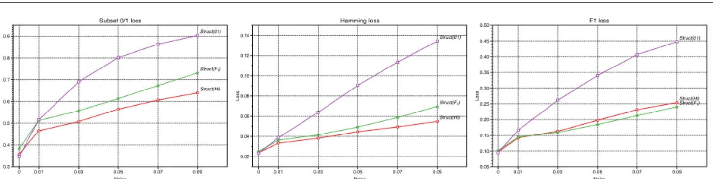
To see at a glance the whole bunch of results, we show Figures 1 and 2. Here we represent the average scores for increasing levels of noise obtained by the learners Struct(Hl), Struct(F1), and Struct(01).
In these figures we see that Struct(Hl) is a quite competitive learner. As expected, it is the best when the purpose is to win in Hamming loss, but the scores obtained with the other performance measures are very good too. In fact, Struct(Hl) outperforms the other op-tions in datasets with some noise when the performance measure is 0/1 loss. InF1, Struct(Hl) outperforms the scores of Struct(F1) when the learning task is easier, with a small proportion of noisy examples. Only when the learning task has high levels of noise, there is a room for improvement: Struct(F1) is better in these cases. Nevertheless, there are no big differences and a tradeoff between performance and algorithmic complexity may be favorable to Struct(Hl).
The competitive performance showed by Struct(Hl) on example-based measures is in line with the results of BR reported in the experimental study [17]. Let us re-call that Struct(Hl) is conceptually equivalent to a BR (Section 2.1) with the only difference that Struct(Hl) performs a combined regularization for all models de-fined in (4).
In general, since the optimization of the Hamming loss produces competitive scores, a simple Binary Rel-evance classifier is useful to solve ML tasks (this con-clusion was also reached in [16]). This is not the case when the aim is to minimize the subset 0/1 loss
with-out noise. In that case the learner optimizing 0/1 loss performs better.
The Appendix at the end of the paper contains a detailed graphical description of the winning regions of each learner in the whole collection of datasets used in the experiments.
7 Conclusions
There is a tradeoff between performance and computa-tional complexity in classification tasks. When the goal is to optimize a loss function defined over the whole classification of a set, as in the F-measures, the learner has to deal with contingency tables. If the aim is to predict a set of labels instead of a single class, the al-gorithms become more complex.
We have presented some contributions to guide the search of a tradeoff in ML classification. On the one hand, we implemented, using a common framework, three learners that explicitly optimize three of the most popular performance measures of ML classifiers, respec-tively: subset 0/1 loss, Hamming loss, and the example-based F-measure. For this purpose we used Structured output Support Vector Machines (SSVM) and extended to ML the method presented by Joachims in [12] to optimize multivariate performance measures. Then, to compare these learners in a wide variety of situations, we used a collection of 528 synthetic ML datasets. Here we included different levels of noise and number of la-bels.
The results of the comparison are detailed in Sec-tion 6 and in the Appendix at the end of the paper.
Table 2 Average train-test results in different noise settings in 528 datasets. The learners used aim to optimizeHamming loss,F1 score, and 0/1 loss. The performance measures are 0/1 loss (0/1), Hamming loss (Hl) and 1−F1. Noise was added
usingBernoulliandSwap(Section 6.1) procedures
Struct(Hl) Struct(F1) Struct(01)
L 0/1 Hl 1−F1 0/1 Hl 1−F1 0/1 Hl 1−F1 Noise free 50 49.39 2.07 14.24 52.04 2.12 14.73 47.70 2.02 14.16 25 36.55 2.52 9.71 39.62 2.60 10.18 35.70 2.46 9.51 10 21.57 2.62 5.18 23.49 2.88 5.63 20.90 2.56 5.02 Bernoulli 0.01 50 62.41 2.88 21.68 71.81 3.35 22.29 75.31 4.03 27.55 25 48.18 3.47 13.81 51.01 3.63 13.65 50.34 3.74 14.66 10 29.02 3.68 7.06 30.94 3.90 7.39 29.03 3.88 7.60 0.03 50 67.86 3.27 25.35 74.52 3.52 23.45 91.45 6.49 41.50 25 51.01 3.81 15.13 55.56 4.05 15.20 76.86 7.14 26.69 10 33.41 4.37 8.39 37.04 4.91 9.12 38.77 5.51 10.29 0.05 50 75.51 3.86 31.43 78.99 4.07 26.38 96.33 8.61 50.96 25 56.68 4.45 17.86 63.00 4.90 18.10 87.58 9.73 34.55 10 37.16 5.09 9.98 41.97 5.82 10.76 56.52 8.85 16.47 0.07 50 79.53 4.15 37.95 84.20 4.76 29.95 98.43 10.28 56.68 25 62.47 5.05 20.40 70.20 5.92 21.34 91.98 11.78 42.77 10 39.92 5.62 11.11 47.56 6.92 12.42 68.50 12.00 22.57 0.09 50 81.05 4.34 39.80 88.73 5.59 33.47 99.56 11.96 61.07 25 66.32 5.63 23.71 75.84 6.90 23.95 95.36 14.17 47.21 10 44.51 6.47 12.80 54.81 8.43 14.80 76.13 14.17 25.96 Swap 0.05 50 56.16 2.43 17.57 60.17 2.54 17.53 53.58 2.30 17.03 25 44.14 3.04 12.30 47.02 3.23 12.54 42.47 2.86 12.16 10 30.37 3.82 7.76 32.68 4.15 7.86 29.91 3.91 7.78 0.1 50 59.51 2.64 19.57 64.09 2.81 19.25 58.70 2.54 19.20 25 48.60 3.41 14.04 51.19 3.56 13.65 47.81 3.48 14.41 10 33.12 4.28 8.74 34.11 4.40 8.35 33.15 4.42 9.00 0.2 50 64.83 2.94 24.09 70.21 3.21 21.66 69.45 3.29 24.95 25 52.71 3.81 16.39 55.15 3.96 14.97 60.08 4.67 19.15 10 36.97 4.96 10.62 39.72 5.39 10.08 48.32 7.20 14.49 0.3 50 68.66 3.16 27.44 74.29 3.58 24.00 79.14 4.19 32.75 25 58.40 4.28 19.55 59.94 4.43 16.97 74.70 6.59 27.76 10 42.29 5.88 12.82 45.85 6.54 11.97 66.74 11.20 23.41 0.4 50 71.69 3.34 30.93 77.16 3.91 25.85 84.42 4.77 37.04 25 61.64 4.59 21.53 62.77 4.83 18.11 77.87 7.22 30.41 10 48.22 7.09 16.09 51.53 7.60 13.67 75.17 13.82 27.01
But the overall conclusions can be summarized in a few words.
In most cases, the optimization of the Hamming loss produces the best or competitive scores. Notice that this is very important in a practical sense since a sim-ple Binary Relevance classifier can be used for this pur-pose. Any binary classifier can be utilized to learn the relevancy of each label separately. Thus, ML tasks can be tackled with a scalable and effective method most of the times.
The limits of this general rule are when the aim is to minimize the subset 0/1 loss in noise-free datasets. In these cases, the specialized learner Struct(01) achieves the best results, although the differences are very small. Bigger differences are appreciated when learning tasks
have high levels of noise and the purpose is to improve the performance in F-measure. In this case the learner that explicitly optimizes this loss outperforms the oth-ers.
Acknowledgements The research reported here is supported in part under grant TIN2011-23558 from the MINECO (Min-isterio de Econom´ıa y Competitividad, Spain), partially sup-ported with FEDER funds. We would also like to acknowl-edge all those people who generously shared the datasets and software used in this paper.
References
1. Cheng, W., H¨ullermeier, E.: Combining Instance-Based Learning and Logistic Regression for Multilabel
Classifi-Struct(Hl) Struct(F1) Struct(01) L o ss 0.3 0.4 0.5 0.6 0.7 0.8 0.9 Noise 0 0.01 0.03 0.05 0.07 0.09 Subset 0/1 loss Struct(Hl) Struct(F1) Struct(01) L o ss 0.02 0.04 0.06 0.08 0.10 0.12 0.14 Noise 0 0.01 0.03 0.05 0.07 0.09 Hamming loss Struct(Hl) Struct(F1) Struct(01) L o ss 0.05 0.10 0.15 0.20 0.25 0.30 0.35 0.40 0.45 0.50 Noise 0 0.01 0.03 0.05 0.07 0.09 F1 loss
Fig. 1 Average scores in datasets with different Bernoulli noise levels (horizontal axis), see Section 6.1. In the leftmost picture we represent 0/1 loss, in the central the Hamming loss, and 1−F1 in the rightmost picture. Since all the scores represent
losses, the lower is the better
Struct(Hl) Struct(F1) Struct(01) L o ss 0.3 0.4 0.5 0.6 0.7 0.8 Noise 0 0.05 0.1 0.2 0.3 0.4 Subset 0/1 loss Struct(Hl) Struct(F1) Struct(01) L o ss 0.02 0.03 0.04 0.05 0.06 0.07 0.08 0.09 Noise 0 0.05 0.1 0.2 0.3 0.4 Hamming loss Struct(Hl) Struct(F1) Struct(01) L o ss 0.10 0.15 0.20 0.25 0.30 Noise 0 0.05 0.1 0.2 0.3 0.4 F1 loss
Fig. 2 Average scores in datasets with different Swap noise levels (horizontal axis), see Section 6.1. In the leftmost picture we represent 0/1 loss, in the central the Hamming loss, and 1−F1 in the rightmost picture. Since all the scores represent losses,
the lower is the better
cation. Machine Learning76(2), 211–225 (2009) 2. Crammer, K., Singer, Y.: On the algorithmic
implemen-tation of multiclass kernel-based vector machines. Jour-nal of Machine Learning Research2, 265–292 (2002) 3. Dembczy´nski, K., Cheng, W., H¨ullermeier, E.: Bayes
op-timal multilabel classification via probabilistic classifier chains. In: Proceedings of the International Conference on Machine Learning (ICML) (2010)
4. Dembczy´nski, K., Kot lowski, W., Jachnik, A., Waege-man, W., H¨ullermeier, E.: Optimizing the f-measure in multi-label classification: Plug-in rule approach versus structured loss minimization. ICML (2013)
5. Dembczy´nski, K., Waegeman, W., Cheng, W., H¨ullermeier, E.: An Exact Algorithm for F-Measure Maximization. In: Proceedings of the Neural Information Processing Systems (NIPS) (2011)
6. Dembczy´nski, K., Waegeman, W., Cheng, W., H¨ullermeier, E.: On label dependence and loss minimiza-tion in multi-label classificaminimiza-tion. Machine Learning pp. 1–41 (2012)
7. D´ıez, J., del Coz, J.J., Luaces, O., Bahamonde, A.: Tensor products to optimize label-based loss measures in multi-label classifications. Tech. rep., Centro de Inteligencia Artificial. Universidad de Oviedo at Gij´on (2012) 8. Elisseeff, A., Weston, J.: A kernel method for
multi-labelled classification. In: Proceedings of the Annual Conference on Neural Information Processing Systems (NIPS), pp. 681–687. MIT Press (2001)
9. Gao, W., Zhou, Z.H.: On the consistency of multi-label learning. Journal of Machine Learning Research - Pro-ceedings Track (COLT)19, 341–358 (2011)
10. Ghamrawi, N., McCallum, A.: Collective multi-label clas-sification. In: Proceedings of the 14th ACM International
Conference on Information and Knowledge Management, pp. 195–200. ACM (2005)
11. Hariharan, B., Vishwanathan, S., Varma, M.: Efficient max-margin multi-label classification with applications to zero-shot learning. Machine learning88(1-2), 127–155 (2012)
12. Joachims, T.: A support vector method for multivariate performance measures. In: Proceedings of the Interna-tional Conference on Machine Learning (ICML) (2005) 13. Joachims, T.: Training linear SVMs in linear time. In:
Proceedings of the ACM Conference on Knowledge Dis-covery and Data Mining (KDD). ACM (2006)
14. Joachims, T., Finley, T., Yu, C.: Cutting-plane training of structural svms. Machine Learning77(1), 27–59 (2009) 15. Lampert, C.H.: Maximum margin multi-label structured
prediction. In: Advances in Neural Information Process-ing Systems, pp. 289–297 (2011)
16. Luaces, O., D´ıez, J., Barranquero, J., del Coz, J.J., Baha-monde, A.: Binary relevance efficacy for multilabel classi-fication. Progress in Artificial Intelligence4(1), 303–313 (2012)
17. Madjarov, G., Kocev, D., Gjorgjevikj, D., Dˇzeroski, S.: An extensive experimental comparison of methods for multi-label learning. Pattern Recognition 45(9), 3084 – 3104 (2012). DOI http://dx.doi.org/10.1016/j. patcog.2012.03.004. URL http://www.sciencedirect. com/science/article/pii/S0031320312001203
18. Monta˜n´es, E., Quevedo, J., del Coz, J.: Aggregating inde-pendent and deinde-pendent models to learn multi-label clas-sifiers. In: Proceedings of European Conference on Ma-chine Learning and Knowledge Discovery in Databases (ECML-PKDD), pp. 484–500. Springer (2011)
19. Monta˜nes, E., Senge, R., Barranquero, J., Ram´on Quevedo, J., Jos´e del Coz, J., H¨ullermeier, E.: Dependent binary relevance models for multi-label classification. Pattern Recognition 47(3), 1494–1508 (2014)
20. Petterson, J., Caetano, T.: Reverse multi-label learning. In: Proceedings of the Annual Conference on Neural In-formation Processing Systems (NIPS), pp. 1912—1920 (2010)
21. Petterson, J., Caetano, T.S.: Submodular multi-label learning. In: Proceedings of the Annual Conference on Neural Information Processing Systems (NIPS), pp. 1512–1520 (2011)
22. Quevedo, J.R., Luaces, O., Bahamonde, A.: Multilabel classifiers with a probabilistic thresholding strategy. Pat-tern Recognition45(2), 876–883 (2012)
23. Read, J., Pfahringer, B., Holmes, G., Frank, E.: Classi-fier Chains for Multi-label Classification. In: Proceed-ings of European Conference on Machine Learning and Knowledge Discovery in Databases (ECML-PKDD), pp. 254–269 (2009)
24. Schapire, R., Singer, Y.: Boostexter: A boosting-based system for text categorization. Machine learning39(2), 135–168 (2000)
25. Tsochantaridis, I., Joachims, T., Hofmann, T., Altun, Y.: Large margin methods for structured and interdependent output variables. Journal of Machine Learning Research
6(2), 1453 (2006)
26. Tsoumakas, G., Katakis, I.: Multi Label Classification: An Overview. International Journal of Data Warehousing and Mining3(3), 1–13 (2007)
27. Tsoumakas, G., Katakis, I., Vlahavas, I.: Mining Multi-label Data. In O. Maimon and L. Rokach (Ed.), Data Mining and Knowledge Discovery Handbook, Springer (2010)
28. Tsoumakas, G., Katakis, I., Vlahavas, I.: Random k-Labelsets for Multi-Label Classification. IEEE Trans-actions on Knowledge Discovery and Data Engineering (2010)
29. Vapnik, V.: Statistical Learning Theory. John Wiley, New York, NY (1998)
30. Vedaldi, A.: A MATLAB wrapper of SVMstruct.
http://www.vlfeat.org/˜ vedaldi/code/svm-struct-matlab.html (2011)
31. Zaragoza, J., Sucar, L., Bielza, C., Larra˜naga, P.: Bayesian chain classifiers for multidimensional classifica-tion. In: Proceedings of the International Joint Confer-ence on Artificial IntelligConfer-ence (IJCAI) (2011)
32. Zhang, M.L., Zhou, Z.H.: ML-KNN: A Lazy Learning Approach to Multi-label Learning. Pattern Recognition
40(7), 2038–2048 (2007)
Appendix
In this section we report the results obtained in the whole collection of datasets. Since we have two differ-ent ways to introduce noise in a learning task (see Sec-tion 6.1), in order to represent all datasets at once, we define thesimilarityof noise free and noisy versions for each dataset and loss or score function. For a loss func-tion∆, the similarity is the complementary of the loss of the noisy release with respect to the noise free output in the test set,
Sim(∆,Y, noise(Y)) = 1−∆(Y, noise(Y)) (9) whereYrepresents the matrix of actual labels. On the other hand, the similarity does not use the complemen-tary inF1,
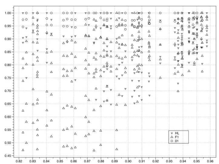
Sim(F1,Y, noise(Y)) =F1(Y, noise(Y)). (10) In Figure 3 each dataset is represented in a 2-dimension space. The horizontal axis represents theF1score achieved by Struct(F1) in the noise free version of the dataset. The vertical axis represents the similarity of the dataset (measured with F1). Thus, points near the top of the picture stand for datasets noise free or datasets with low noise. On the other hand, points near the left side rep-resent harder datasets, in the sense that the noise free releases achieves lowerF1scores. Finally, the points in this space are labeled by the name of the learner that achieved the bestF1 score.
Here we observe that Struct(F1) outperforms the other learners in terms ofF1when tackling harder learn-ing tasks (left bottom corner of Figure 3). In easier tasks, mainly those with 10 or 25 labels, the procedure (Algorithm 2) seems to require more evidences in order to estimate the optimal expected F1. In any case, the differences in the easiest learning tasks are small.
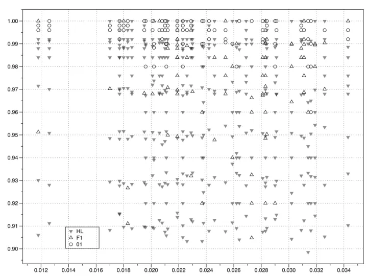
To complete the discussion of the results, we made figures analogous to Figure 3 using subset 0/1 loss (Fig. 4), and Hamming loss (Fig. 5).
HL F1 01 0.45 0.50 0.55 0.60 0.65 0.70 0.75 0.80 0.85 0.90 0.95 1.00 0.82 0.83 0.84 0.85 0.86 0.87 0.88 0.89 0.90 0.91 0.92 0.93 0.94 0.95 0.96
Fig. 3 Learners winning inF1score in the 528 datasets. The horizontal axis represents theF1score of datasets in the noise
free releases. Thus points at the right hand side stand for easier datasets, typically those with less number of labels. The vertical axis represent the similarity of label sets, usingF1similarity (10), with the noise free version. The higher the points
HL F1 01 0 0.1 0.2 0.3 0.4 0.5 0.6 0.7 0.8 0.9 1.0 0.15 0.20 0.25 0.30 0.35 0.40 0.45 0.50 0.55 0.60 0.65 0.70
Fig. 4 Learners winning in 0/1lossin the 528 datasets. The horizontal axis represents the 0/1lossof datasets in the noise free releases. Thus points at the left hand side stand for easier datasets, typically those with less number of labels. The vertical axis represent the similarity of label sets, using 0/1 similarity (9), with the noise free version. The higher the points in the figure, the lower the noise in the datasets
HL F1 01 0.90 0.91 0.92 0.93 0.94 0.95 0.96 0.97 0.98 0.99 1.00 0.012 0.014 0.016 0.018 0.020 0.022 0.024 0.026 0.028 0.030 0.032 0.034
Fig. 5 Learners winning inHamming lossin the 528 datasets. The horizontal axis represents the Hamming loss of datasets in the noise free releases. Thus points at the left hand side stand for easier datasets, typically those with less number of labels. The vertical axis represent the similarity of label sets, using Hamming loss similarity (9), with the noise free version. The higher the points in the figure, the lower the noise in the datasets