A scalable implementation of information theoretic feature selection for high dimensional data

A Scalable Implementation of Information Theoretic

Feature Selection for High Dimensional Data

Anthony Kleerekoper

, Michael Pappas

, Adam Pocock

, Gavin Brown

, Mikel Lujan

∗

_{School of Computing, Mathematics and Digital Technologies, Manchester Metropolitan University, UK}

_{School of Computer Science, The University of Manchester, UK}

‡

_{Oracle Labs, Burlington, MA}

selection is a vital component of machine learning as well as an important stand alone data analytics tool. Without it, the computation cost of big data analytics can become unmanageable and spurious correlations and noise can reduce the accuracy of any results. Feature selection removes irrelevant and redundant information leading to faster, more reliable data analysis.

Feature selection techniques based on information theory are among the fastest known and the Manchester AnalyticS Toolkit (MAST) provides an efficient, parallel and scalable implemen-tation of these methods. This paper considers a number of data structures for storing the frequency counters that underpin MAST. We show that preprocessing the data to reduce the number of zero-valued counters in an array structure results in an order of magnitude reduction in both memory usage and execution time compared to state of the art structures that use explicit mappings to avoid zero-valued counters.

We also describe a number of parallel processing techniques that enable MAST to scale linearly with the number of processors even on NUMA architectures. MAST targets scale-up servers rather than scale-out clusters and we show that it performs orders of magnitude faster than existing tools. Moreover, we show that MAST is 3.5 times faster than a scale-out solution built for Spark running on the same server. As an example of the performance of MAST, we were able to process a dataset of 100 million examples and 100,000 features in under 10 minutes on a four socket server which each socket containing an 8-core Intel Xeon E5-4620 processor.

Keywords—Big Data, Data Analytics, Data Structures, Feature Selection, Information Theory, Mutual Information, Parallel Pro-cessing

I. INTRODUCTION

Feature selection is a component of machine learning and can also be used as a stand alone data analytics tool [1]. It identifies the parts of the data that are relevant to the knowledge we seek and separates those parts from other irrelevant or redundant parts. With the growth of data with very high dimensionality, feature selection is becoming a critical step in big data analytics. Without using feature selection, the high dimensionality results in greatly increased computation costs as well as undermining the accuracy of analysis because of noise accumulation and spurious correlations [2].

Fortunately, in many large data sets a very large propor-tion of the features are not relevant [3]. Feature selecpropor-tion can greatly reduce the dimensionality of the data without

Dr Pocock’s work on this project was completed whilst he was at the University of Manchester.

compromising analytical accuracy by removing irrelevant or redundant features. Unfortunately, the high dimensionality of the data that makes feature selection so necessary also affects feature selection itself. Fast feature selection techniques are needed and filter methods are the fastest techniques as they are independent of any machine learning algorithm and rely only on correlations inherent in the data [4], [5] (Section II-A). A large number of filter methods are based on information theory, specifically mutual information, to mathematically evaluate the relevance and redundancy of data [6], [7] (Section II-B). As well as using inherently faster methods, optimising their implementation through efficient parallelisation is also crucial. In this paper we describe an efficient, parallel and scalable implementation of information theoretic operations as well as some of the most popular filter methods, part of the Manch-ester AnalyticS Toolkit (MAST). We consider the question of which data structure to use to minimise memory use and execution time. A basic building block of information theoretic operations is the maintenance of a large number of counters that store the number of times combinations of feature values appear in the data. There is a trade-off between implicitly and explicitly storing the mapping from the keys (feature values) to the counters. If we store the mapping implicitly (e.g. in arrays) then we can have faster access times but may have to store zero-valued counters. On the other hand, an explicit mapping never has to store zero-valued counters but has increased access times (Section III).

In this paper we propose pre-processing steps to reduce the number of zero-valued counters needed when using an implicit mapping. We show that the resulting data structure, which we call a tokenised array, uses an order of magnitude less memory and is an order of magnitude faster than using standard explicit mappings such as hash tables and balanced binary trees (Section IV). We also describe some of the parallelisation techniques used to ensure that MAST scales linearly with the number of threads even on NUMA (Non-Uniform Memory Access) server architectures (Section V).

MAST targets scale-up servers rather than scale-out clus-ters. Recently, it has been observed that the majority of big data analytics problems running on clusters are in the order of 10s to 100s of Gigabytes and would therefore benefit more from scale-up than scale-out [8], [9]. Compared to existing tools that target single servers, MAST is orders of magnitude faster even over small datasets. MAST is also capable of handling very large datasets whereas existing tools could not process more than 100,000 examples on our machine. We also compare MAST to an existing information theoretic feature selection

package released recently for Spark [10] and find that MAST is more than 3.5 times faster (Section VI).

II. FEATURESELECTION

A. Feature Selection Techniques

The data used for feature selection is commonly formatted as a two-dimensional matrix of values where each row rep-resents one example and each column represents onefeature. Every example is associated with a class label which is the value that learning algorithms aim to predict.

With the growth of big data - specifically high dimensional data - it is becoming challenging to apply traditional machine learning techniques. Not only is the computation time greatly increasing but the quality of the models generated by the machine learning algorithms are reduced by the plethora of features. Spurious relationships can emerge as simple artefacts of the data which are statistically true but reveal no true knowledge about the underlying system [2], [3].

In this context, feature selection is vital because it identifies a subset of the features that are actually relevant to the class label. Consider, for example, a data set concerning the price of cars. We know by experience which features are likely to be relevant (e.g. the mileage) and which are likely to be irrelevant (e.g. the colour of the wheel trim). In some cases a feature may become redundant in the presence of another, for example we might not need to know the age of a car if we know its mileage. In more complex datasets or those for which we have little experience we must rely on automated, statistical methods.

In many high-dimensional data sets, a majority of the features are actually irrelevant [3]. Feature selection can iden-tify a subset of features that are, ideally, the most relevant, but it is clearly impossible to consider every possible subset and therefore greedy methods are used. Typically this process either starts with no features and adds one per iteration up to some maximum (forward selection) or else starts with all the features and removes one per iteration up to some minimum (backwards elimination) [11]. In all cases, scores must be assigned to subsets in order to rank them and either add or remove the appropriate features.

In general there are two approaches to assigning these scores: wrapper and filter methods. In wrapper methods the score is based on the accuracy of a given machine learning algorithm. The algorithm is trained on each subset and the resulting model is used to predict the values of the class labels for some testing data. The score for the given subset is the accuracy or error of those predictions. In filter methods the scoring function is independent of any learning algorithms. Instead, each subset is given a score based on statistical relationships between the features and the class labels.

Because filter methods do not include any machine learning algorithm during their calculation of the scores they are known to be the fastest methods [4], [5]. They rely on identifying statistical relationships between the features and the class labels such as correlations. Simple linear correlation tests, such as Pearson’s, are limited in their ability to discern relationships. As an alternative, methods using mutual information, have emerged as the prime filter methods. Recently, more than 15 such techniques have been brought together under a common

mathematical framework as approximate iterative maximisers of the conditional likelihood [6], [7].

B. Calculating Mutual Information

Mutual information is a way of quantifying the amount of information that one random variable contains about another. Another way of putting it is that the mutual information is the information contained in one variable that is revealed by a second one.

In information theory, the amount of information contained in a variable is measured by its entropy,H(X). Entropy can also measure the information of a variable conditioned on a second, H(X|Y), which measures the amount of information contained in a variableX given that we know all the informa-tion contained inY. Mutual information measures the amount of information that is common to two variables. It is therefore defined as the difference between the total information of a variable and the information of that variable condition on a second variable. That is, the mutual information is:

I(X;Y) =H(X)−H(X|Y).

In terms of probabilities, if the variable X has values

{x1, x2. . . xi}, the probability that a sample ofX has value

xi isp(xi)and the mutual information is defined as:

I(X;Y) =X ij p(xi, yj) log _p(x i, yj) p(xi)p(yj) . (1)

It is also possible to extend this idea to joint mutual in-formation which gives a measure of the inin-formation contained by a pair of variables about a third.

The feature selection component of MAST currently offers a number of methods including Conditional Mutual Informa-tion MaximisaInforma-tion (CMIM) [12] and Max-Relevance Min-Redundancy (MRMR) [13]. MAST also provides APIs for information theoretic values which facilitates the addition of further methods.

III. STORINGFREQUENCYCOUNTERS

From Equation (1) in the previous section, we see that in order to calculate mutual information we estimate the probability of every combination of feature and label values. That is, for every pair of features X and Y with label

L, we need to estimate the probability of the combination (xi, yj, lk). An effective method of estimating this probability

is to adopt the histogram method based on counting the frequency of occurrences in the data [14]. This method is especially appropriate for big data because of the Strong Law of Large Numbers which tells us that as we have more examples the probability estimate converges almost surely to the true probability.

Because probability estimates are required so frequently, MAST provides data structures called

jointRandomVariable objects (jrv) that store the

frequency counts and provide information theoretic measures. We handle the process of reading and processing the data and

TABLE I. SUMMARY OF THE THREE DATA STRUCTURES WE CONSIDER FOR STORING THE COUNTERS

Data Structure Mapping Type Access Time Memory Requirement

Array Implicit O(1) O(n)

Hash Table Explicit O(1) on average O(n) Balanced Binary Tree Explicit O(log n) O(n)

the jointRandomVariable objects provide interfaces for

other modules to make efficient use of the processed data. Thejrvobjects constitute the main memory use because if there aremfeatures then(m2_{−m)/2jrvobjects are needed} (i.e. the number of pairs of melements without repetition). A crucial question, therefore, is which data structure for storing the counters results in the fastest execution time and least memory usage. In the remainder of this section we describe the trade-offs involved and the preprocessing steps we take to produce an efficient structure that we call a tokenised array. A. Data Structure Trade-off

Each counter stores the frequency for a given combination of feature and label values and can therefore be though of as a <key, counter> pair where the key is of the form (xi, yj, lk). There is a choice between explicitly or implicitly

storing the mapping between keys and counters. Explicitly storing the mapping may result in additional processing time for updates and inserts, but it ensures that we never store zero-valued counters – i.e. counters for a combination of values that never appear in the data. On the other hand, implicitly storing the mapping can reduce the processing time but potentially requires storing zero-valued counters in order to maintain the mapping.

For example, suppose that in a given dataset the valid values of feature X are {1,2,4} and for feature Y they are

{1,2,3}. An implicit mapping might store the counters in the following key order: (1,1), (2,1), (3,1), (4,1) (for convenience we do not include the label values). Although the key (3,1) can never appear in the data because 3 is not a valid value for featureX, there is no way to know this in advance. Therefore, the counter corresponding to key (3,1) must be stored in order to maintain the mapping. In contrast, if we store the keys explicitly then we would not store an entry for key (3,1) because it would never appear in the data.

We consider two standard data structures that explicitly store keys but have fast average access times: hash tables and balanced binary trees (in the form of Red-Black Trees). Both offer O(n) space requirements wherenis the number of items being stored but differ slightly in their time complexity. Hash tables have constant amortised access times but can have O(n) time in the worst case. Balanced binary trees have O(logn) access times in both the average and worst case. For implicit mappings we consider an array-based structure which has constant access times (see Section III-B for details). The three structures are summarised in Table I.

Another difference, aside from their time complexities, is the constant overhead of identifying a counter given a key. For arrays, the mapping is implicit and so the key value directly provides an index into the array. Hash tables have higher overheads because of the need to compute the hash function to find the counter address from the key. Balanced binary trees

also have higher overheads because the tree is traversed by comparing keys.

Therefore, the trade-off is between potentially storing un-necessary zero-valued counters but having fast access times and having slower access times but never storing unnecessary data. In the remainder of this section we describe preprocessing steps we can take to reduce the number of zero-valued counters stored in an array, which we then call a tokenised array. B. Preprocessing for Tokenised Arrays

We have seen that there is a trade-off between storing zero-valued counters and access time. Updating and later accessing counter values is the dominant operation of MAST which might lead us to assume that the reduced overhead of arrays makes it the best choice. However, the problem of zero-valued counters is potentially extremely severe.

Zero-valued counters can appear for two reasons. The first is that a particular combination of values simply does not appear in the data. The second is that a particular combination of values is not valid, as in the key (3,1) in the earlier example. We cannot prevent the first but we can preprocess the data to prevent the second.

The second cause of zero-valued counters is potentially far more severe because the valid values for a given feature can be any set of discrete values 1. For implicit mapping to work we have to be able to use the values of the features to directly index the array. However, we do not know the valid values of a feature when creating the arrays and therefore, we have no choice but to have the lowest index as 0. If, in fact, the smallest valid value for a feature is a large integer then we will have to “pad” the entire range of invalid values with zero-valued counters. Moreover, the valid values need not be consecutive integers meaning that we may have to pad within the range of valid values. These problems are so severe that, depending on the data, we may consume the entire memory of any machine with only zero-valued counters.

For example, consider a dataset in which a given feature can only have values {15,30,45,60}. Since we have no way of knowing in advance that the smallest value is 15, we have no choice but to store counters corresponding to keys 0-14 even though they will all be zero-valued. Similarly, we cannot know that there are no valid keys in the ranges 16-29, 31-44 and 46-59 and so we store a large number of zero-valued counters.

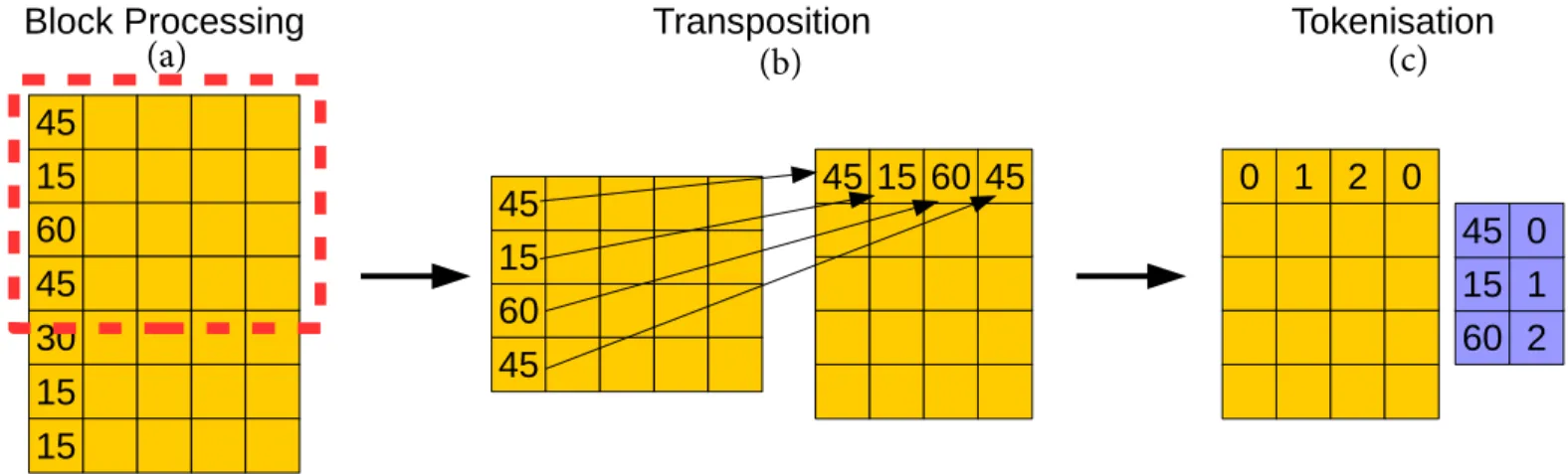
To avoid this problem we propose two preprocessing steps to remove the second cause of zero-valued counters and thereby make arrays a feasible choice for storing counters. The two steps aretokenisationandtranspositionand are illustrated in Fig. 1.

The aim of tokenisation is to translate the true valid values of a feature into a set of “tokens” which is a contiguous set of integers beginning with 0. During tokenisation, the true values of each feature are read and compared to a stored mapping of values to tokens (see Fig.1(c)). If the value has been seen before then it is replaced with the corresponding token, if not, a new token is generated and a new mapping is created 1_{A discretisation tool is included with MAST to preprocess real-valued data}

30

15

15

45

60

15

45

45

60

15

45

45 15 60 45

0 1 2 0

60 2

15 1

45 0

Block Processing

Transposition

Tokenisation

(a)

_(b)

(c)

Fig. 1. Data is preprocessed for tokenised arrays in three steps. First the data is read in blocks. Those blocks are then transposed so that the consecutive values of the same feature are in contiguous blocks of memory. Finally the feature values are converted into “tokens” which are consecutive integers.

and then the value is replaced with the new token. For our example, if the original values were{45,15,15,60,30,30,45}

the corresponding tokens would be {0,1,1,2,3,3,0}. For all subsequent operations the tokens are used and not the original values. This does not affect the correctness of the program, but has the advantage that the tokens can be used to directly index the tokenised array. The only zero-valued counters that will be stored are those corresponding to cases where a combination of values is simply missing in the data, which we cannot know in advance.

There are two inefficiencies with tokenisation. The first is that we must store the mapping between original values and tokens and this brings us back to the same problem we are trying to solve with the counters. We note, however, we need far fewer such mappings. Whilst we needO(m2_)jrvobjects for m features we only need O(m) mappings for the tokens. Moreover, eachjrvobject containsO(n3_{)keys if each feature} and the label has n valid values whereas each set of tokens contains onlyO(n)keys.

The second problem is the time required to preprocess all the data and tokenise it. Since the tokenisation process is independent for each feature we note that it is perfect parallelism. However, the benefit of parallelisation is hindered by the format of the data. Consecutive values of a given feature are separated by the values of all the other features and therefore there could be potentially long strides leading to poor performance. We therefore introduce a second preprocessing step before tokenisation which we calltransposition.

In transposition the layout of the input data is changed so that each row now contains all the values of a given feature (see Fig. 1(b)). Consecutive feature values will therefore be in a contiguous block of memory which will enhance performance, assuming a C-array layout.

Since the data may be very large we cannot efficient trans-pose the entire dataset in one go and therefore we use block processing during transposition, tokenisation and updating the counters. A relatively small number of examples are read in a block and then processed before the next block is read (see Fig. 1(a)). This avoids the danger of filling memory with the data and having to offload some of it to disk during transposition and tokenisation.

TABLE II. THE TWO MACHINES WE USED FOR TESTING # Sockets Processors per Socket Main Memory Operating System

Machine A 1 4-core Intel Core i5-760 6GB Ubuntu 13.04 Machine B 4 8-core Intel Xeon E5-4620 264GB Ubuntu 12.04 LTS

Fig. 2. The peak memory usage with arrays was consistently an order of magnitude lower than with either of the alternative storage methods.

IV. COMPARINGDATASTRUCTURES

In the previous section we introduced the three data struc-tures for storing counters and the preprocessing steps required for tokenised arrays. Here we show that the tokenised array results in an order of magnitude reduction in both memory and execution time compared to the alternatives - despite the added overhead of preprocessing the data. The hash table structure was implemented with the unordered_map container and the balanced binary tree structure was implemented with the

map container from the Standard Template Library [15]. A. Memory Usage

The memory usage of MAST is determined primarily by the number of features which determines how many jrv

objects there will be. The number of examples is important only in as much as we need to create counters for every combination of feature values. If there is only a small number

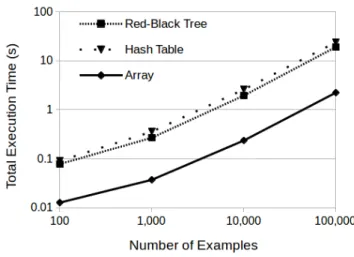
Fig. 3. The execution time of MAST increases exponentially with the number of features but is approximately an order of magnitude faster with the chosen storage system than with the alternatives.

of examples then many combinations may not appear in the data. As the number of examples increases the likelihood of seeing every valid combination at least once increases. For each new valid combination a new counter is needed (at least when keys are stored explicitly) but once all the counters have been created any increase in the number of examples does not affect the memory usage. Since our primary interest is for big data we may reasonably expect to have a large number of examples relative to the number of features and therefore we only show results for the effect of the number of features.

To test the memory requirements of MAST with the three structures we ran the feature selection tool using Valgrind’s massif tool and recorded the peak memory usage [16]. The experiments were run on Machine A in Table II.

In the first experiment we fixed the number of examples at 100,000 and varied the number of features, always selecting 10%. The results in Fig. 2 show (on a log-log scale) that the memory requirement grows quadratically with the number of features since we have(m2_{−m)/2jrvobjects formfeatures.} The array method uses approximately an order of magnitude less memory than the alternatives which both have very similar usage. The difference grows as the number of features grows, starting at approximately 7.5 times less memory with only 10 features and rising to approximately 40 times and then 50 times less with 1,000 features.

B. Execution Time

The results in Fig. 2 show that the tokenised array struc-ture results in significantly less memory usage than with the alternatives. Here we consider whether the preprocessing that reduces the memory leads to increased execution time.

Fig. 3 shows the results when varying the number of features. The overall execution time of MAST increases quadratically with the number of features because the number of pairs of features is proportional to the square of the number of features. When using the tokenised array structure, the exe-cution time is approximately an order of magnitude faster than when using the other structures. The preprocessing required for

Fig. 4. The execution time of MAST increases linearly with the number of examples but is approximately an order of magnitude faster with the array data structure than with the alternatives.

the array structure turns out to be very fast, corresponding to less than 5% of the total execution time even for very small datasets and less than 1% for larger ones. Since updating and accessing the counters is the dominant operation, the faster operations of the tokenised array more than compensates for the preprocessing time.

When varying the number of examples, Fig. 4 shows that the execution time increases linearly. This is because the total execution time is dominated by the time to update the counters which is linear in the number of examples. The array structure results in an order of magnitude speedup over the other methods because of its lower overhead.

V. OVERALLSCALABILITY

As well as performing tokenisation in parallel, we have also implemented the updating of the counters and calculation of mutual information in parallel. Here we present experimental results showing the impact of some of the optimisations and of the overall scalability of the parallelisation. All of the experiments in this section were conducted on our scaled-up server, Machine B in Table II.

A. Avoiding mallocLocks

We implement parallelism throughout by parsing, transpos-ing, tokenistranspos-ing, updating the counters and selecting the features in parallel. Many of the stages require malloc operations to alter data structure sizes during processing. For example as new values are seen that have to be given new tokens or when thejrvobjects must grow bigger to accommodate new, unseen tokens. Since the memory being assigned is shared there is contention between threads requiring locks in order to avoid errors. These locks can cause significant overhead during parallel processing.

One way around this problem would be to pre-scan the entire dataset so that the required sizes of all data structures is known in advance. However, this approach is certainly not suitable for big data because of the size of the datasets involved. Doing nothing, however, is also not a viable option

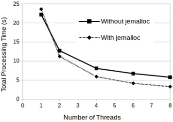
Fig. 5. jemalloc brings a small overhead which causes additional processing time during single-threaded execution but brings significant benefits during multi-threaded execution.

Fig. 6. MAST scales very well on a single socket using the optimisations. Here the results are for selecting 100 features from a datset of 1,000 examples and 1,000 features.

because we are likely to have a very large number ofmalloc

operations and the overheads will become very significant. MAST therefore makes use of the open-sourcejemalloc

package which provides an alternative implementation of

malloc designed to reduce the overhead of shared memory

accesses [17]. Fig. 5 shows the impact of using jemalloc

within MAST. It brings some added overhead which causes a small increase in execution time when only a single thread is being used but for multiple threads it results in significant im-provements. Indeed, the relative improvement of jemalloc

over malloc increases as the number of threads increases

from 1.1 times speedup with 2 threads to 1.75 with 8. B. Overall Scalability

Fig. 6 shows the scaling of the total execution time for a relatively small dataset consisting of 1,000 rows and 1,000 features. In the example 10% of the features are selected which means that the execution time is split approximately 70%-30%

Fig. 7. The scaling of MAST improves as the data becomes more complex because the overheads become less significant.

between selecting the features and updating the counters. The scaling for the feature selection part of the program (FS) is slightly better than for the updating time (JRV) and therefore the scaling overall is in between these two, slightly closer to FS than JRV.

The optimisations and parallelism have resulted in scaling that is close to linear even for this relatively small dataset. The main reason for not achieving ideal, linear speedup is that there is overhead in creating and destroying threads during execution which increases with more threads. With larger datasets, however, those constant overheads become increasingly insignificant and the scalability asymptotically approaches the ideal linear speedup.

C. NUMA Architecture

Scale-up servers are most likely to have not just multiple cores but multiple sockets and adopt the NUMA (Non-Uniform Memory Access) architecture. In the NUMA architecture, main memory is physically divided and distributed among the sockets. Each socket has a direct connection to the memory “attached” to it but must use interconnects with the other sockets to access the other parts of main memory. Access to the attached memory is significantly faster than to other parts, hence the name non-uniform memory access.

In NUMA machines there is often a first-touch policy which means that a newly created object or data read from disk is placed into the main memory attached to the socket whose CPU created or read the data. If a different CPU on a different socket wants to access that data it must access it through the first socket and this can create a bottleneck. To solve this problem, MAST creates objects in parallel so that they are better spread among the sockets. The increased overhead of creating threads to create objects is more than compensated by the faster memory accesses during the course of the program’s execution.

Fig. 7 shows how MAST scales on a NUMA server with four sockets and 32 cores in total. When more threads are being used there is significant overhead which causes the speedup to slow down. Nevertheless, as the number of features increases the scaling increases, approaching the ideal, linear speedup. Of

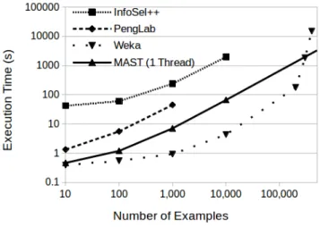
Fig. 8. Even when only using a single thread MAST is at least two orders of magnitude of faster than InfoSel++ and at least one order of magnitude faster than PengLab.

course, it is precisely with larger datasets that scaling becomes more important and we show that it can approach near-ideal scaling when the overheads of multi-threaded processing become less important.

VI. COMPARISON WITHRELATEDWORK

A. Scale-Up

There are a number of existing tools and programs that can perform feature selection on scale-up servers. Here we briefly describe the tools most similar to our own and show their limitations in terms of information theoretic feature selection (see Fig. 8).

Weka:Weka is the premier program for machine learning produced by the University of Waikato [18]. The program is primarily aimed at performing machine learning but also has the capability of performing feature selection (which they call attribute selection) and a number of approaches are provided. In all there are 11 search methods available with 17 scoring functions although not all are available for every data set. Additional methods can be added from external packages. Weka contains only one feature selection method based on mutual information, called InfoGain, which ranks features based on their mutual information with the class label.

PengLab: PengLab is a feature selection tool produced by Hanchuan Peng which implements his proposed MRMR algorithm [13].

InfoSel++:InfoSel++ is the newest tool and is designed for information based feature selection [19]. It consists of a series of C++ libraries with more than twenty selection methods and is intended to facilitate rapid prototyping of new methods. InfoSel++ can also be used as a stand alone program.

We compared MAST to Weka, InfoSel++ and PengLab on Machine A (see Table II), a standard desktop. Since InfoSel++ and PengLab are only capable of single-threading we ran MAST in single-thread mode, even though this negates the parallelism built in to the framework.

Fig. 8 shows the execution times of the four tools for datasets of 1,000 features with varying number of examples on a log-log scale. The results show the limitations of the alternative tools. PengLab failed for datasets with more than 1,000 examples and InfoSel++ failed for those with more than 10,000. Weka ran out of Java heap memory during its execution of a dataset with 400,000 examples after running for more than 4 hours (the heap size was set to the maximum of 6GB). In contrast, MAST was able to perform feature selection on datasets up to 1 billion examples without memory issues.

The results also show that MAST is an order of magnitude faster than InfoSel++ and up to six times faster than PengLab, even though it was only using a single thread which negated many of its improvements. Weka, by contrast is faster than single-threaded MAST for small datasets but for large data becomes slower.

We note, however, that the comparison between MAST and Weka is not a direct comparison of the same algorithm. The information theoretic scoring function available in Weka only considers the mutual information between each feature indvidualy and the class label. It does not consider joint mutual information between pairs of features or between pairs of features and the label. Therefore, it is not as complex as the feature selection algorithms implemented in MAST, performing approximately m times less work where m is the number of features. We include the comparison only for completeness.

These results therefore illustrate the gulf in performance between MAST and the alternative feature selection tools targeted at single machines rather than clusters.

B. Scale-Out

A number of machine learning packages have been created for scale-out clusters. Mahout offers a platform for scalable machine learning algorithms [20]. It includes matrix decom-position techniques for feature selection but not any based on information theory. MLLib offers feature selection using the Chi Squared method which tests for the independence of the features with the class label but does not take into account the relationship between features [21].

Recently, information theoretic feature selection methods have been implemented for Spark [10]. In our experiments we found that this implementation was unable to process a dataset with 5,000 features. We compared MAST with the Spark implementation on a dataset with 1 million examples and only 1,000 features, both running on Machine B (Table II) with Spark running standalone with one job per core. The Spark implementation took 1,038 seconds whereas MAST took 289 seconds to process the dataset, a speedup of more than 3.5 times.

VII. CONCLUSIONS

Feature selection is vital for analytics of data with very high dimensionality. Without it, the computational cost is extremely high and spurious correlations can affect the validity of results. Information theoretic feature selection methods are among the fastest known methods and the Manchester AnalyticS Toolkit (MAST) provides an efficient, parallel and scalable implementation of the most popular such methods.

Information theory relies on probability estimation which can be done effectively through the use of frequency counters. In this paper we considered which data structure for storing counters results in the smallest use of memory and execution time. We consider the trade-off involved in the choice between implicitly or explicitly storing the mapping from feature values to counters. We show that by transposing and tokenising the input data we can use an array-based structure which reduces memory usage and execution time by an order of magnitude compared to hash tables or balanced binary trees.

MAST also implements its stages in parallel, adding an additional transposition stage to rearrange the data in memory to facilitate parallel tokenisation. By transposing the data, consecutive feature values are in contiguous memory blocks. Furthermore, MAST uses the open-sourcemallocalternative,

jemalloc, to provide memory allocation that is better suited to parallel programming.

Experimental results show that these optimisations have extremely significant impact on the scalability of MAST. When the number of threads is small, MAST has almost linear scaling with the number of threads. On NUMA architectures, with more threads and more overhead, MAST’s scalability is hampered but as the number of features increases it approaches linear scaling.

On a standard desktop and limiting MAST to a single thread, we found that MAST is an order of magnitude faster when compared to the most similar alternative, InfoSel++, and many times faster than PengLab. Moreover, MAST was able to handle very large datasets whereas InfoSel++, PengLab and even Weka, failed to handle larger datasets. As an example of possible performance, MAST was able to compute a solution to a dataset of 100 million examples and 100,000 features in under 10 minutes using 32 threads on four 8-core Intel Xeon E5-4620 processors.

MAST targets scale-up servers as recently it has been observed that a large number of big data analytics jobs are more suited to scale-up servers than scale-out clusters. Many scale-out packages do not offer information theoretic feature selection and one recent offering was unable to match the performance of MAST. Nevertheless, there will certainly be situations where scale-out is necessary. We believe that the optimisations and methods included in MAST for scale-up can be successfully applied to scale-out to provide an efficient and scalable implementation for extremely large data.

Another area of future work is to consider advanced data structures for storing the counters. These structures can offer sublinear memory requirements by only maintaining approx-imations to the true counts. Early work suggests that these structures may be useful for the probability estimation task [22].

ACKNOWLEDGMENT

The research leading to these results has received funding from the European Union’s Seventh Framework Programme (FP7/2007-2013) under grant agreement 318633 and from the EPSRC under grants PAMELA EP/K008730/1 and AnyScale Applications EP/L000725/1. M. Lujan is funded by a Royal Society University Research Fellowship.

REFERENCES

[1] Isabelle Guyon and Andr´e Elisseeff. An introduction to variable and feature selection.The Journal of Machine Learning Research, 3:1157– 1182, 2003.

[2] Jianqing Fan, Fang Han, and Han Liu. Challenges of big data analysis.

National science review, 1(2):293–314, 2014.

[3] Mingkui Tan, Ivor W Tsang, and Li Wang. Towards ultrahigh dimen-sional feature selection for big data.The Journal of Machine Learning Research, 15(1):1371–1429, 2014.

[4] Noelia S´anchez-Maro˜no, Amparo Alonso-Betanzos, and Mar´ıa Tombilla-Sanrom´an. Filter methods for feature selection–a comparative study. InIntelligent Data Engineering and Automated Learning-IDEAL 2007, pages 178–187. Springer, 2007.

[5] Ver´onica Bol´on-Canedo, Noelia S´anchez-Maro˜no, and Amparo Alonso-Betanzos. A review of feature selection methods on synthetic data.

Knowledge and information systems, 34(3):483–519, 2013.

[6] Gavin Brown. A new perspective for information theoretic feature selection. In International Conference on Artificial Intelligence and Statistics, pages 49–56, 2009.

[7] Gavin Brown, Adam Pocock, Ming-Jie Zhao, and Mikel Luj´an. Condi-tional likelihood maximisation: A unifying framework for information theoretic feature selection.The Journal of Machine Learning Research, 13:27–66, 2012.

[8] Antony Rowstron, Dushyanth Narayanan, Austin Donnelly, Greg O’Shea, and Andrew Douglas. Nobody ever got fired for using hadoop on a cluster. InProceedings of the 1st International Workshop on Hot Topics in Cloud Data Processing, page 2. ACM, 2012.

[9] Raja Appuswamy, Christos Gkantsidis, Dushyanth Narayanan, Orion Hodson, and Antony Rowstron. Nobody ever got fired for buying a cluster. Technical report, Technical Report MSR-TR-2013-2, Microsoft Research, 2013.

[10] Sergio Ramrez-Gallego, Hctor Mourio-Taln, and David Martnez-Rego. An information theoretic feature selection framework, 2015.

[11] Rich Caruana and Dayne Freitag. Greedy attribute selection. InICML, pages 28–36. Citeseer, 1994.

[12] Franc¸ois Fleuret. Fast binary feature selection with conditional mutual information.The Journal of Machine Learning Research, 5:1531–1555, 2004.

[13] Hanchuan Peng, Fuhui Long, and Chris Ding. Feature selection based on mutual information criteria of max-dependency, max-relevance, and min-redundancy. Pattern Analysis and Machine Intelligence, IEEE Transactions on, 27(8):1226–1238, 2005.

[14] David W Scott. Multivariate density estimation: theory, practice, and visualization. John Wiley & Sons, 2015.

[15] Phillip James Plauger, Meng Lee, David Musser, and Alexander A Stepanov.C++ Standard Template Library. Prentice Hall PTR, 2000. [16] Nicholas Nethercote, Robert Walsh, and Jeremy Fitzhardinge. Building workload characterization tools with valgrind. In IEEE International Symposium on Workload Characterization (IISWC 2006), October 2006. [17] Jason Evans. A scalable concurrent malloc (3) implementation for freebsd. InProc. of the BSDCan Conference, Ottawa, Canada. Citeseer, 2006.

[18] Mark Hall, Eibe Frank, Geoffrey Holmes, Bernhard Pfahringer, Peter Reutemann, and Ian H Witten. The weka data mining software: an update. ACM SIGKDD Explorations Newsletter, 11(1):10–18, 2009. [19] Adam Kachel, Jacek Biesiada, Marcin Blachnik, and Włodzisław Duch.

Infosel++: Information based feature selection c++ library. InArtificial Intelligence and Soft Computing, pages 388–396. Springer, 2010. [20] Sean Owen, Robin Anil, Ted Dunning, and Ellen Friedman.Mahout in

action. Manning Shelter Island, 2011.

[21] Xiangrui Meng, Joseph Bradley, Burak Yavuz, Evan Sparks, Shivaram Venkataraman, Davies Liu, Jeremy Freeman, DB Tsai, Manish Amde, Sean Owen, et al. Mllib: Machine learning in apache spark. arXiv preprint arXiv:1505.06807, 2015.

[22] Anthony Kleerekoper, Mikel Luj´an, and Gavin Brown. Exploring sketches for probability estimation with sublinear memory. InBig Data, 2013 IEEE International Conference on, pages 79–86. IEEE, 2013.