Distributed Algorithms on Exact Personalized PageRank
Tao Guo
1Xin Cao
2Gao Cong
1Jiaheng Lu
3Xuemin Lin
21School of Computer Science and Engineering, Nanyang Technological University, Singapore 2School of Computer Science and Engineering, The University of New South Wales, Australia
3Department of Computer Science, University of Helsinki, Finland
[email protected], [email protected], [email protected], [email protected], [email protected]
ABSTRACT
As one of the most well known graph computation problems,
Per-sonalized PageRankis an effective approach for computing the
similarity score between two nodes, and it has been widely used in various applications, such as link prediction and recommendation. Due to the high computational cost and space cost of computing the exact Personalized PageRank Vector (PPV), most existing studies compute PPV approximately. In this paper, we propose novel and efficient distributed algorithms that compute PPV exactly based on graph partitioning on a general coordinator-based share-nothing distributed computing platform. Our algorithms takes three aspects into account: the load balance, the communication cost, and the computation cost of each machine. The proposed algorithms only require one time of communication between each machine and the coordinator at query time. The communication cost is bounded, and the work load on each machine is balanced. Comprehensive exper-iments conducted on five real datasets demonstrate the efficiency and the scalability of our proposed methods.
1.
INTRODUCTION
Measuring the similarities between nodes is a fundamental graph computation problem. Many random surfer model based meas-ures have been proposed to capture the node-to-node proximities [2, 9, 24, 25, 30]. ThePersonalized PageRank(PPR) [25] is one of the most widely used measures and has gained extensive attention because of its effectiveness and theoretical properties. It has been utilized in various fields of applications, such as web search [8,11], community detection [3, 21], link prediction [4], anomaly detec-tion [43], and recommendadetec-tion [22, 27].
Different from thePageRankmodel [38], PPR allows users to specify a set of preference nodesP. The result of PPR w.r.t.Pis called the Personalized PageRank Vector (PPV), which is denoted byrP. Note that different preference vectors will yield different
PPVs, and thus PPV needs to be computed in an online manner, which is different from PageRank. The PPR model can be sim-ulated by numerous “random surfers.” Initially, these surfers are distributed to the nodes inPequally. Next, in each step, a random surfer either jumps to a random outgoing neighbor with a
probab-ility of1−α, or teleports back to a nodeuinPaccording to the specified preference ofuwith a probability ofα(αis called the
teleport probability). The procedure is performed repeatedly until
it converges to a steady state, i.e, the number of surfers on each node does not change after each iteration. The final distribution of the random surfers on the nodes represents the PPV ofP.
The PPR model can also be interpreted as a linear system. We denoteuPas the preference vector w.r.t. PandAas the
normal-ized adjacency matrix of the graph. PPVrP can be computed as:
rP= (1−α)ATrP+αuP. (1)
Hence,rPcan be computed using the power iteration method, i.e., rkP+1 = (1−α)A
T
rkP+αuP, whererkP represents the vector
computed in thekthiteration, andr0
Pis set to a uniform
distribu-tion vector. Finally,rPconverges to the PPV ofP.
A. Challenges. Although computing PPVs has been extensively
studied since the problem is first proposed in the work [25], it is still a very challenging task to compute exact PPVs efficiently for different online applications. One straightforward method is to ad-opt the power iteration approach by following Equation 1, which is however computationally expensive, and it is not practical for the online applications of PPR.
In the work [25], the linearity property of PPV is studied for computing PPVs exactly. If we pre-compute the PPV for each node, at query time, given a node setP, according to the property, the PPV ofP can be constructed using the pre-computed PPVs of the nodes inP. Unfortunately, this method is impractical be-cause of both the expensive pre-computation time and the offline storage requirements (whereO(|V|2)
space is needed). In order to reduce the complexity and space cost, the work [25] selects some important nodes as the “hub nodes”, and the user preference nodes can only be from the hub set, thus losing the generality. Due to the hardness of computing the exact PPVs, most of existing studies (e.g., [5,14,44,49]) focus on computing approximate PPVs. These methods sacrifice the accuracy to accelerate PPV computation.
Facing the challenges of computing the exact PPV for any ar-bitrary user preference node set, a natural question raised is how to perform the computation in parallel on multiple machines to gain efficiency. However, it is known that graph algorithms often exhibit poor locality and incur expensive network communication cost [34]. Therefore, it is a challenging task to design an efficient and scalable distributed algorithm for computing PPVs that has low communication cost and is able to achieve load balance.
The power iteration method can be implemented on the gen-eral distributed graph processing platforms to compute PPVs in a distributed way. However, this would not be suitable because of the unavoidable high communication cost. In the power iteration method, computing the vector in the current iteration requires the
vector of the previous iteration. Thus, no matter how we distrib-ute the computation, one machine always has to ask for some data from the other machines in each iteration before convergence, thus incurring expensive network communication cost. For example, the graph processing engine Pregel [36] is based on the general bulk synchronous parallel (BSP) model [45]. In each iteration of the BSP execution, Pregel applies a user-defined function on each vertex in parallel. The communications between vertexes are per-formed with message passing interfaces. The block-centric system Blogel [47] distributes subgraphs to machines as blocks, and mes-sages between blocks are transmitted over the network. Both Pre-gel and BloPre-gel need many rounds of communications to compute PPVs, which incurs expensive communication cost, thus suffering from low efficiency.
B. Our Proposal. In this work, we design novel distributed
al-gorithms utilizing the graph partitioning for computing exact PPVs, which can be implemented on a general coordinator-based share-nothing distributed computing platform. We take into account three aspects in designing our algorithms: the load balance, the commu-nication cost, and the computation cost on each machine. A sali-ent feature of the proposed algorithms is that each machine only needs to communicate with the coordinator machine once at query time, and we prove that the communication cost of our method is bounded. The main idea of our algorithms are outlined as below.
Observation 1: We can separate the graph into disjoint subgraphs
of similar size to distribute the PPV computation.
Based on this observation, we propose thegraph partition based
algorithm, denoted byGPA. We prove that the benefit from the
bal-anced disjoint graph partitioning is two-fold: first, this guarantees a total space cost ofO((|V|−|H|)2/m+2|V||H|+|H|2
)), whereV
represents the nodes of the graph,mis the number of subraphs, and
Hrepresents the set of hub nodes separating the subgraphs. Note that|H|is much smaller than|V|(see more analysis in Appendix E), and thus this space cost is significantly smaller than applying the method [25] directly. Second, this enables us to compute PPVs in parallel on separate machines without incurring communication cost between machines. At query time, based on the pre-computed values, each machine constructs part of the PPV, and only commu-nicates with the coordinator once (i.e., sending part of the PPV to the coordinator). If we usenmachines, the communication cost of GPAisO(n|V|).
Observation 2: We notice that if we treat each subgraph as an indi-vidual graph, we can useGPAto compute the “local” PPV of each node w.r.t. the subgraph itself, and these local PPVs can be used to construct the final “global” PPV. This motivates us to further parti-tion each subgraph and we get a tree-like graph hierarchy. Then, we can recursively applyGPAalong the hierarchy of subgraphs. We prove that the pre-computation space cost can be further reduced and bounded by utilizing the graph hierarchy.
Observation 3: Since the sizes of subgraphs in different levels of the hierarchy are different, simply distributing the subgraphs to ma-chines cannot achieve load balance. We design a method to distrib-ute the PPV computation evenly based on hub nodes partitioning to solve this problem.
Based on the aforementioned observations, we propose the
hier-archical graph partition based algorithm, denoted byHGPA, which
greatly reduces the space cost, and we prove that the communica-tion cost ofHGPAisO(n|V|)as well.
C. Contributions. To the best of our knowledge, this is the first work that is able to compute exact PPVs efficiently in a distributed manner with reasonable space cost. In this paper, we propose novel distributed algorithms based on graph partitioning, and the salient features of new algorithms can be summarized as follows:
• Efficiency: Our proposed algorithm HGPAis10 ∼ 100
times faster than the power iteration approach running on general distributed graph processing platforms Pregel+ [48] and Blogel [47], and can meet the efficiency need of online applications. The experimental study also shows thatHGPA is faster than the power iteration and one state-of-the-art ap-proximate PPV computation algorithm [49] even under the centralized setting.
• Accuracy: Our proposed algorithms, namelyGPAandHGPA,
are able to obtain the same result as that of the work [25], and thus have guaranteed exactness (Theorems 1 and 3).
• Load Balance: Our distributed algorithmsGPAandHGPA
are load balanced andHGPAscales very well with both the size of datasets and the number of machines. As shown in the experiments, the runtime can be reduced nearly by half if we double the number of machines.
• Low Communication Cost: Our algorithms only require
one time of communication between each machine and the coordinator, and no communication between any two ma-chines is needed for pre-computation and query processing. As shown in the experiments, our method only costs about 1.5 MB network communication to compute a PPV on a graph containing 3M nodes using 10 machines.
The rest of the paper is organized as follows. Section 2 provides the preliminary of this work. Sections 3 and 4 present the distrib-uted algorithmsGPAandHGPA, respectively. Section 5 explains our distributed pre-computation. We perform comprehensive ex-periments to evaluate the efficiency and scalability of our meth-ods on 5 real datasets, and the results are reported in Section 6. Section 7 summarizes the related work on computing personalized PageRank. Finally, Section 8 offers conclusions and future research directions.
2.
PRELIMINARY
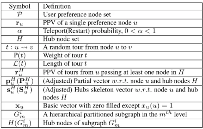
Table 1: Definition of main symbols.
Symbol Definition
P User preference node set
ru PPV of a single preference nodeu
α Teleport(Restart) probability,0< α <1
H Hub node set
t:u v A random tour from nodeutov
P(t) Weight of tourt
L(t) Length of tourt
rH
u PPV of tours fromupassing at least one node inH
pH
u(PHu) (Adjusted) Partial vectorw.r.t.nodeuand hub nodesH
sHu(SHu) (Adjusted) Hubs skeleton vectorw.r.t.nodeuand hub
nodesH
xu Basic vector with zero filled exceptxu(u) = 1
Gi
m A hierarchical partitioned subgraph in themthlevel
H(Gi
m) Hub nodes of subgraphGim
2.1
PPV Decomposition
As proved by Jeh and Widom [25], the PPV scoreru(v)is equal to the correspondingInverse P-distancefrom a query nodeutov, which is measured by all the weighted tours fromutov:
ru(v) = X
t:u v
P(t), (2)
where each tourt:u vrepresents a random surfer that consists of a sequence of edges starting fromuand ending atv. Note that it is allowed to teleport back tou, and thus there may exist cycles in
the tour. The weight of a tourP(t)is the probability that this tour walks fromutovalong witht:
P(t) =α(1−α)L(t) L(t) Y i=1 1 |Out(wi)| ,
where nodesw1(i.e., u), w2,· · ·, wL(t)(i.e., v)comprise the path
of lengthL(t), and|Out(wi)|is the outdegree of nodewi. Al-though the concept of inverse P-distance intuitively explains the distribution of random walk, it is impossible to sum up all the tours to obtain the PPV values. The reason is that there may exist loops in the tours, and thus the number of tours could be infinite.
In order to computeru, it is divided into two types of vectors w.r.t. a set of hub nodesH, i.e., partial vectors and hubs skeleton vectors.
Definition 1: Partial vector: Given a nodeu, itspartial vector
pH
u is defined as a vector of random walk results computed using tours passing through no hub nodes. That means, given a nodev,
pHu(v) =
X
∀w∈t&w6=u,w /∈H
P(t)
Definition 2: Hubs skeleton vector: Given a node u, itshubs
skeleton vectorsHu is defined as a vector of|H|dimensions
com-posed of all hub nodes’ PPV values w.r.t. u. Given a hub nodeh,
sHu(h) =ru(h).
u1
u2
u3
u4 u5
Figure 1: Random Surfer Example
If a tour passes no hub node, it contributes to the partial vector. If a tour stops at a hub node, it contributes to the skeleton vector. For ease of understanding, we explain the meaning of the two types of vectors with the graph shown in Figure 1, where two nodesu2
andu3are selected as hub nodes. We next illustrate the partial and
skeleton vectors with nodeu1as an example.
The partial vectorpHu1 consists of two tourst1 andt2, where
t1 = u1 u4 andt2 = u1 u4 u5. Note that all other
tours are blocked by eitheru2oru3(hub nodes), and thus any gray
node in this example is not reachable fromu1. We havepHu1(u4) =
P(t1)andpHu1(u5) =P(t2).
For the skeleton vectorsHu1, we only consider the tours stopping at a hub node. Different from the partial vector, the tour can contain one or more hub nodes. Fromu1to hub nodeu2, there exist two
tourst3 =u1 u2andt4=u1 u4 u5 u2. Fromu1to
u3there exist three tourst5 =u1 u2 u3,t6 =u1 u4
u5 u3, andt7 = u1 u4 u5 u2 u3. Therefore, sHu1(u2) =P(t3) +P(t4)ands
H
u1(u3) =P(t5) +P(t6) +P(t7). Note that because of cycles in the tours, it is not feasible to com-pute all possible tours, which may be infinite. This simple example is only used to illustrate the intuitive meaning of the two types of vectors.
2.2
PPV Construction
The PPV ofu(i.e.,ru) can be constructed by the partial vectors and hubs skeleton vectors. We userH
u to denote the vector of ran-dom walk results computed using tours passing though at least one hub node. That is, give a nodev,rHu(v) =
P
t:u H vP(t). We
can combinerH
u and the partial vector ofuto obtain the full PPV ofu:rHu +puH =ru. As proved by Jeh and Widom [25],rHu can be computed according to the following equation:
rHu = 1 α X h∈H (sHu(h)−αfu(h))·(pHh −αxh), (3) wherefu(h) =1 ifu=h, and 0 otherwise.fu(h)is used to deal with the special case when uis a hub node. xhis a vector that has value 1 athand 0 everywhere else. It is used to deal with the special case whenhis the target node.
In order to make the equations more clear, we define theadjusted
partial vectorfor each hub nodeh:
PHh =p H
h −αxu,
and theadjusted hubs skeleton vectorSHu for each nodeu, where:
SHu(h) =s H
u(h)−αfu(h).
After the partial vectors and skeleton vectors have been pre-computed, the exact PPV of a given query nodeucan be construc-ted by: ru= 1 α X h∈H SHu(h)·P H h +p H u (4)
In order to reduce the complexity, the work [25] only considers the construction of PPV for hub nodes. According to Equation 4, we need to pre-compute the partial vectors of all hub nodes, which requires space costO((|V| − |H|)· |H|)in the worst case, and the skeleton vectors of all hub nodes, which requiresO(|H|2
)space.
2.3
A Brute-force Extension
It is too restricted to consider the hub set from only preference nodes as done in work [25]. In fact, it can be extended to com-pute the PPV for any given query node, as indicated by Equa-tion 4. However, it incurs huge space cost as explained below: first, pre-computing the partial vectors for non-hub nodes requires worst case space costO((|V| − |H|)2), which happens when every
node can reach every other node without passing any hub node; second, pre-computing the partial vectors for hub nodes requires
O((|V| − |H|)|H|)space in the worst case; third, pre-computing the skeleton vectors for all nodes requires space costO(|V| · |H|). Thus, the total pre-computation space cost isO(|V|2
), which is equivalent to pre-computing the PPVs of all nodes. In practice, the vectors may be sparse and the space cost is usually not that large, but it is still not applicable for large graphs. We denote this al-gorithm byPPV-JW.
3.
ALGORITHM
GPA
Although it is usually difficult to efficiently parallelize graph al-gorithms [34], we propose thegraph partition based algorithm, de-noted byGPA, to distribute the PPV computation. We present the algorithm details in Section 3.1. We adopt a general coordinator-based share-nothing distributed computing platform. For the con-venience of presentation, we call each machine handling some sub-graphs as “machine” and the machine aggregating the final result as “coordinator.” In addition, in Section 3.2 we prove thatGPA re-duces the space cost significantly compared with the method PPV-JWpresented in Section 2.3.
3.1
Distributed PPV Construction
Graph partition is commonly used in parallel computing [23], but it is always challenging to decouple the computation dependencies. We aim to distribute the PPV computation to multiple machines and each machine can independently compute part of the result.We
use a balanced graph partition algorithm (METIS [26]) to divide the graph intomdisjoint subgraphs. Figure 2 shows an example, where the graph is partitioned into two disjoint subgraphsG1and
G2. The bridging nodes between subgraphs form the hub nodes. In
the example,u1andu2are selected as the hub nodes.
After the graph is partitioned intomsubgraphs, we distribute the subgraphs to multiple machines evenly. The pre-computed partial vector and skeleton vector of each node is stored in the machine where the node resides.
u1 u 3 u2 u4 u5 G1 G2 Figure 2: Example of graph partition and hub nodes Recall that the PPV construction of the method [25] is based on Equation 4. Now the pre-computed vectors are stored onn ma-chinesM1, ...,Mn, and we can distribute the computation accord-ing to the followaccord-ing equation:
ru= 1 α n X i=1 X h∈H(Mi) SHu(h)·P H h +p H u, (5)
whereH(Mi)denotes the set of hub nodes assigned toMi. Assume that the partial and skeleton vectors have already been pre-computed and stored. We introduce the details of this step in Section 5. Equation 5 indicates that we can do the distributed PPV construction at query time as follows: after a query nodeu
is given, the coordinator first detects the machineMuthat stores the partial vector ofu. Then,Mucomputes the following vector:
vu=α1 Ph∈H(Mu)S
H
u(h)·PHh +pHu. Simultaneously, each of the other machinesMj(1 ≤ j ≤ n, j 6= u) computes a vector
vj = α1Ph∈H(Mj)S
H u(h)·P
H
h. The coordinator receives the vectors computed from all machines, and computes the final PPV asru =Pni=1vi. Therefore, at query time, each machine com-municates with the coordinator exactly once.
Theorem 1:GPAcan obtain the same results as computed by the
work proposed by Jeh and Widom [25]. PROOF. Pni=1P
h∈H(Mi)is equal to
P
h∈H, and thus Equa-tion 5 can compute the same vector as EquaEqua-tion 4.
Communication Cost. Each machine needs to compute a vector
of size|V|, and then sends it to the coordinator. Thus, ifn ma-chines are employed inGPA, the total communication cost ofGPA isO(n|V|).
Time Complexity. According to Equation 5, to compute a node
u’s PPV, we need to fetch the partial vector of each hub nodeh
reachable from nodeu(i.e., PHh), the skeleton vector ofu(i.e.,
SH
u), and the partial vector ofu(i.e.,PHu). The partial vector of each hub nodehgets its weightSHu(h)from the skeleton vector of
u, and they are then aggregated together withPHu. Therefore, we need to read at mostO(|H|)vectors of dimension|V|andO(|H|) vectors.
Assume that we usenmachines and the hub nodes are distrib-uted evenly to these machines. In the worst case, on each machine we only need to sum upO(|H|/n)vectors, and on the coordin-ator we need to sum upnvectors. Thus, the complexity of GPA is
O(1n|H||V|+n|V|).
3.2
Space Cost of
GPA
We proceed to show that the space cost ofGPAis reduced signi-ficantly compared withPPV-JW, the extension of the method [25] as presented in Section 2.3. We use an example as shown in Fig-ure 2 to briefly explain the reason. In the work [25], nodes with high PageRank values are chosen as hub nodes, since most random walks have high probability to visit these nodes. As a result, nodes
u1 andu3are selected to be the hub nodes. The support of
vec-torpHu4 (the partial vector ofu4) can be as large as the size of the graph, since there exists a tour fromu4 to each other node in the
graph. If we select the nodesu1 andu2 as the hub nodes, they
are able to partition the graph into two disjoint subgraphs. In this way, every tour from nodeu4to a node in the other part has to pass
eitheru1oru2, and thus the tours between different subgraphs are
blocked by the hub nodes. The support ofpHu4 is reduced to the size of the subgraph containingu4.
As illustrated in the example, after the graph partition, we select the bridging nodes between subgraphs as the hub nodes. The ran-dom walks that represent partial vectors are restricted within each individual subgraph by the hub nodes. Thus, the support of the partial vector of non-hub nodepHu is reduced from|V| − |H|to the size (the number of nodes) of the subgraph containingu. In PPV-JW, the space cost of partial vectors of non-hub nodes, i.e.,
O((|V| − |H|)2), is the major cost. InGPA, if we assume that the graph is partitioned intomsubgraphs of equal size, the size of each subgraph isO((|V| − |H|)/m), and the space cost isO((|V| − |H|)2/m). In the worst case, the space cost of storing the partial vectors of the hub nodes isO((|V|−|H|)|H|), and storing the skel-eton vectors of non-hub nodes costsO(|V||H|). In conclusion, the total space cost ofGPAisO((|V| − |H|)2/m+ 2|V||H| − |H|2
), based on the balanced graph partition.
Note that for most graphs, the number of hub nodes that can divide the graphs into different components is always much smaller than the total number of nodes, i.e.,|H| |V|. Therefore, the space cost ofGPAis much smaller thanO(|V|2
), the cost of PPV-JWto compute PPV for an arbitrary node in a centralized setting.
4.
ALGORITHM
HGPA
InGPA, the computation of partial vectors is restricted to each individual subgraph, and the total space cost of all machines is con-sequently reduced compared with that required by the centralized extension of the method [25]. To further reduce the space cost and achieve better load balance and efficiency, we propose a new ap-proach based on a hierarchy of subgraphs. This algorithm is in-spired by the observation that, the computation of a nodeu’s par-tial vector is equivalent to the computation of the “local” PPV ofu
w.r.t. the subgraph that containsu.
We first introduce how we can compute the partial vectors us-ing the way of computus-ing “local” PPVs in Section 4.1. Based on this property, we partition the graph into a hierarchy of subgraphs as presented in Section 4.2. Then, we introduce how to get PPV utilizing the graph hierarchy in Section 4.3, and we design the dis-tributed PPV computation method to achieve load balance in Sec-tion 4.4. We prove that the space cost benefits from the hierarchical graph partitioning in Section 4.5.
4.1
Partial Vector vs Local PPV
InGPA, we partition the graph into disjoint subgraphs. Recall that as presented in Section 2 PPV can be computed by the random surfers following all possible paths, and the partial vector of a node is the result computed using random surfers passing no hub node. Therefore, the computation of the partial vector of a node is only related to the subgraph containing the node. This motivates us to
u1 u3 u2 u4 u5 u6
Figure 3: Full GraphG
u
4u
5u
6Figure 4: SubgraphSG
think whether it is possible to use the local PPV of a node w.r.t. a subgraph to compute the partial vector of this node. Consider the toy graph in Figure 3, which is separated by hub nodeu2. Figure 4
shows the isolated subgraphSG. Suppose the query node isu5, we
would like to know whether the partial vectorpH
u5inGis equal to the local PPV ofu5inSG, i.e.,ru5[SG].
Recall that the computation ofP(t)requires the out-degrees of nodes in the tourt. The out-degree ofu5 is2in Gbut it is1
in subgraphSG, and obviously the probability of a random surfer walking fromu5 tou4 is different in the two graphs. Therefore, pHu5 6=ru5[SG]. In order to solve this problem, we introduce the following definition.
Definition 3: Virtual subgraph: After partitioning a graph into
smaller subgraphs, for each subgraphSG, we create a virtual node VN, and for each edge that connects a hub node and a nodeuin
SG, we create an edge betweenuand VN. We call the graph composed of subgraphSGand its virtual node as well as the edges connecting them thevirtual subgraph, which is denoted bygSG.
u
4u
5u
6Figure 5: Virtual SubgraphgSG
Figure 5 shows the corresponding virtual subgraph of SGas shown in Figure 4. Using the concept of the virtual subgraph, we have the following theorem.
Theorem 2:Given a graphG, a set of hub nodesH, and a nodeu
in a subgraphSG, the partial vector ofu, i.e.,pH
u is equivalent to
u’s PPV vector w.r.t. the virtual subgraph ofSG, i.e.,ru[gSG]. PROOF. Given any node vin G, the value ofpHu(v) can be computed using the tours fromutovwithout passing through any hub node inH. Ifv /∈ SG,pH
u(v) = 0. Otherwise,pHu(v)= P
t:u vP(t)wheret:u vrepresents a tour fromutovwithin
SG.
According to Equation 2,ru[gSG](v)can also be computed by P
t:u vP(t). Note that all tours are withingSG, the virtual node ingSGhas no outgoing edge. Hence, for each tourt, the value of P(t)is the same for computing bothpHu(v)andru[gSG](v), and this means thatpHu(v)is equal toru[gSG](v).
Using virtual subgraphgSG, we guarantee that the partial vec-tor equals to the local PPV in the virtual subgraph, i.e.,pHu5 =
ru5[gSG]. For the simplification of presentation, we use “subgraph” to indicate “virtual subgraph” in the rest of the chapter.
4.2
Hierarchical Graph Partitioning
Based on Theorem 2, we can obtain the partial vector for a node by computing the local PPV in the subgraph containing the node.
To compute the local PPV for a subgraph, we can recursively apply GPAwithin the subgraph, i.e., we further partition the subgraph into lower level subgraphs, and for each lower level subgraph we apply Theorem 2, and the procedure can be repeated until we hit a specified level. To realize the idea, we recursively partition the whole graph from top to down into a hierarchy. For ease of present-ation, we partition the graph into a hierarchy of two-way partitions. As shown in Figure 6, the root of the hierarchy isGitself. Gen-erally, in themth (0 ≤ m ≤ l) level,Gis partitioned into2m disjoint subgraphs, and we denote a subgraph in themthlevel by
Gi
m, where0≤i <2m. In this hierarchy, given a subgraphGim, its parent subgraph isGb
i
2c
m−1, and its two child subgraphs areG 2i
m+1
andG2mi+1+1. We denote the hub nodes separatingG 2i m+1andG2mi+1+1 byH(Gi m). ... ... ... ... ... ... ... ... ... 0 1 G G11 i m G 2 / 1 i m G i m G2 1 211 i m
G
) ( i m G HG
Figure 6: Hierarchy of the original graph
Figure 7 exemplifies the hierarchy and the hub nodes of each level obtained using the multilevel 2-way partitioning method. First,
Gis partitioned intoG01andG11. At this level, edges (u2, u4) and
(u2, u5) are hub edges, and we can get the hub node setH(G) =
{u2}. In the next level, G01 is partitioned intoG02 and G12 with
no hub node;G11is partitioned intoG22 andG32with hub node set
H(G1
1) ={u4}. Note that once a node is selected as hub node, this
node and all the related edges will be omitted in the next level and not appear in any of the subgraphs. For example,u2is contained
inH(G)but in neitherG0 2norG12.
u
1u
3u
2u
4u
5G
10G
11G
20G
21G
23G
22u
6Figure 7: Example of the hierarchy
We use the two-way partitioning to reduce the number of hub nodes. We employ the 2-way partitioning algorithm [26] to recurs-ively perform the partitioning from top to down, until we reach a level such that no edges exist within the same subgraph. Us-ing the two-way partitionUs-ing, minimizUs-ing the number of hub nodes is identical to the minimum vertex cover problem in a bipartite graph. This problem is proved to be solvable in polynomial time by K˝onig’s theorem [33]. We use the algorithm [33] to select the
minimum hub nodes from the returned hub edges. Our proposed techniques are still applicable if we adopt multiple-way partition-ing. We compare the effects of different partitioning strategies in Section 6.
4.3
PPV Construction on Hierarchy
We proceed to explain the procedure of PPV computation based on the hierarchy. Consider the hub nodes setH0in the first level of
the hierarchy, which separatesGinto two subgraphsG0 1andG11.
Given a query nodeu∈G11, according to Equation 4, to obtainru inGPA, we need the partial vector of nodeu, i.e.,pH0
u , the partial vectors of hub nodes, i.e.,pH0
h (h∈ H0), and the skeleton vectors sH0
u .
pH0
h ands
H0
u can be computed similarly as inGPA. According to Theorem 2, the partial vector ofu(pH0
u ) is identical tou’s PPV vector w.r.t. the virtual subgraph ofG11. Thus, we can compute
the local PPV ofuw.r.t. Gf1
1 asp H0
u . That is, we constructp
H0 u by using the local skeleton vector of lower leve hub nodes inGf11 and the local partial vector ofuinGf11, which can be further com-puted based on lower level subgraphs, and thus the procedure can be repeated until we reach the leaf-level subgraphs.
Assume that all partial and skeleton vectors have been processed and stored (see more details in Section 5). Formally, the construc-tion at query time can be described by the following equaconstruc-tion:
ru= l−1 X m=0 1 α X h∈H(G(mu)) SHu[G (u) m ](h)·PHh[G (u) m ] +ru[G(lu)], (6)
whereG(mu) denote the subgraph in themthlevel that containsu,
SH
u[G
(u)
m ]is the adjusted skeleton vector ofuw.r.t. the subgraph
G(mu), andPHh[G
(u)
m ]is the adjusted partial vector of a hub node w.r.tG(mu). Note that the subgraphs we visit areG(lu),G
(u)
l−1,G (u)
l−2,
· · ·,G0
0, and thus the number of graphs visited during this
proced-ure is exactlyl.
Theorem 3:The vector computed by Equation 6 is exactly the
same as that computed byGPA.
PROOF. u’s local partial vector at levelmcan be computed as:
ru[G(mu)] = 1 α X h∈H(G(mu)) SH u[G (u) m ](h)·PHh[G (u) m ] +ru[G(mu−1) ].
Therefore, Equation 6 can be written as:
ru= l−2 X m=0 1 α X h∈H(G(mu)) SHu[G (u) m ](h)·PHh[G (u) m ] +1 α X h∈H(G(lu−1)) SH u[G (u) l−1](h)·PHh[G (u) l−1] +ru[G(lu)] = l−2 X m=0 1 α X h∈H(G(mu)) SHu[G (u) m ](h)·PHh[G (u) m ] +ru[G(l−1u)] =· · · = 1 α X h∈H(G(0u)) SHu[G (u) 0 ](h)·P H h[G (u) 0 ] +ru[G(1u)]
Note thatG(0u)is the whole graph, andG(1u)can be viewed as a subgraph inGPA, and thus the result of Equation 6 is exactly the same as Equation 5.
4.4
Distributed PPV Computation
Based on the graph hierarchy, we can compute the PPV of a graph from the pre-computation results w.r.t. its hub nodes and the PPV of its child graphs. However it is still challenging to design a distributed algorithm, especially when the graph is large and the pre-computation vectors are too large to save in memory.
To address these challenges, we proposeHGPA, the hub-distributed hierarchical graph partition based algorithm, which is load bal-anced and scalable because the computation in each level can be evenly distributed. We use one coordinator machine to collect the results from other machines forHGPA. We note that the computa-tion ofrurelies on all hub nodes in all levels as shown in Equa-tion 6. This inspires us to divide the hub node set of each subgraph in each level into disjoint components to distribute the computa-tion. Specifically, given a subgraphSG, we divideH(SG)intos
disjoint subsets equallyH1(SG), H2(SG),· · ·, Hs(SG), where
H(SG) = ∪s i=1H
i
(SG). We do this on each subgraph in each level. As a result, the computation ofrucan be interpreted as Equa-tion 7 based on the balanced hub nodes partiEqua-tion.
ru= l−1 X m=0 1 α s X i=1 X h∈Hi(G(mu)) SuH[G(mu)](h)·PHh[Gm(u)] +ru[G(lu)] (7)
It is obvious that the first component of Equation 7 can compute the same results as the first component in Equation 6.
Based on Equation 7, for each subgraph in each level, we divide its hub node set evenly intosdisjoint subsets and store them ins
machines. We also distribute the leaf level subgraphs evenly tos
machines. Each machine only maintains the partial and skeleton vectors of nodes stored on it. Given a query nodeu, theith ma-chine computes a vector using the pre-computation results stored on it, i.e.,P h∈Hi(G(mu))S H u[G (u) m ](h)·PHh[G (u)
m ], and then sends the vector to the coordinator. The partial vectors of all non-hub nodes w.r.t. their leaf level subgraphs (e.g.,ru[G
(u)
l ]) are also dis-tributed to s machines evenly. The coordinator sums up all the vectors received from the machines to construct the PPV. Figure 8 illustrates the idea ofHGPA.
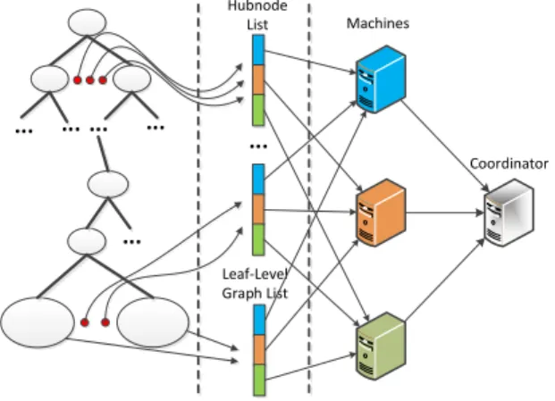
... ... ... ... ... Hubnode List ... Leaf-Level Graph List Machines Coordinator
Figure 8:HGPAArchitecture
It is obvious that algorithmHGPAis load balanced. The compu-tation on each machine is presented by Algorithm 1.
Theorem 4:If the hub node set of each subgraph is divided inton
disjoint subsets, the communication cost can be bounded byO(n|V|). PROOF. InHGPA, each machine computes a vector of size at
Algorithm 1:HGPAprocessor(q,i,α) 1 ppv~ ←~0;
2 foreachsubgraphGsdo
3 foreachhubnodehinHi(Gs)do
4 foreachnon-zero entrypH
h[Gs](k)do
5 ppv(k)~ ←ppv(k) +~ SH
q[Gs](h)·PHh[Gs](k)/α;
6 ifqis not a hub node andPH
q[G
q
l]on machineithen
7 foreachnon-zero entryPH
q(k)do
8 ppv(k)~ ←ppv(k) +~ PH q [Gql](k);
9 sendppv~ to coordinator;
most|V|, and sends it to the coordinator. Hence, the total commu-nication cost isO(n|V|).
4.5
Space Cost of
HGPA
We assume that the graph is partitioned in balance in each level. Letldenote the level of the graph hierarchy, and there are2lleaf level subgraphs. We have the following theorem that shows the space complexity ofHGPA.
Theorem 5: The space cost ofHGPAisO((|V| − |H|)2/2l+ Pl
i=0|Hi|(|V|−|H|)/2
i
+(|V|−|H|)Pli=0|Himax|), whereHi is the set of hub nodes in theithlevel, andHimaxis the maximum number of hub nodes in a subgraph in theithlevel.
PROOF. In the leaf level, we compute and store the PPV of non-hub nodes w.r.t. each subgraph, and the size of the local PPV is (|V| − |H|)/2l. Therefore, the total space cost of storing PPVs for leaf level subgraphs isO((|V| − |H|)2/2l)).
In theithlevel, there are2isubgraphs. For each subgraphGji, we need to compute the partial vectors of the hub nodes in it. Hence, the space cost of storing the partial vectors of hub nodes for the level isO(|Hi|(|V| − |H|)/2i). For all levels, the total space cost of this part isO(Pli=0|Hi|(|V| − |H|)/2i).
We also need to compute the skeleton vectors of the non-hub nodes inGji, and the space cost forG
j
iisO((|V|−|H|)/2 i|
Hi(Gji)|), whereHi(Gji)is the set of hub nodes inG
j i. In thei
th
level, in total the space cost isO((|V| − |H|)/2iP2i
j=0|Hi(Gij)|)< O((|V| −
|H|)/2iP2i
j=0|H
max
i |) =O((|V| − |H|)|Himax|). Thus, for all levels, the total cost of this part isO((|V|−|H|)Pli=0|Himax|).
To compare the space cost ofGPAwithHGPAin an intuitive way, we consider that inGPAthe graph is partitioned as the leaf level of the graph hierarchy inHGPA, i.e., the leaf level subgraphs inHGPAare the subgraphs inGPA. We can conclude thatHGPA has smaller space cost thanGPA. The two algorithms have the same space cost of storing the partial vectors of non-hub nodes. How-ever,HGPAhas smaller space cost of storing the partial vectors of hub nodes and the skeleton vectors of non-hub nodes than that in GPA, becauseO(|V||H|) > O(Pli=0|Hi|(|V| − |H|)/2i)and
O((|V| − |H|)|H|)> O((|V| − |H|)Pli=0|Hmax
i |).
5.
DISTRIBUTED PRE-COMPUTATION
We proceed to present how to pre-compute the partial and the skeleton vectors in a distributed manner for our algorithms.
5.1
Distributed Partial Vectors Computation
We adopt theselective expansion algorithm[25] as introduced in Section E.1 to compute the partial vectors for all nodes. As shown in Equation 9, the iteration requires the information of the graph
structure. We keep a copy of the graph structure on each machine. As a result, no communication is required in the pre-computation of partial vectors. The computation can be done for each node sep-arately, and each machine only needs to handle the nodes assigned to it.
InGPA, each machine only computes the partial vectorpHu if nodeuis assigned to it. When computing the partial vectors for a non-hub node, only the structure of the subgraph containing the node is required, because the computation can be restricted by the subgraph.
InHGPA, the partial vectors of nodes are computed by doing iterations w.r.t. the subgraphs, rather than w.r.t. the whole graph as inGPA, thus reducing the space and time complexity required during the iteration for a node. Given a nodeuassigned to machine
M, ifuis a non-hub node,Mcomputes its partial vector w.r.t. the leaf-level subgraph containingu. Otherwise, ifuis a hub node at levelm,M computes its partial vector w.r.t. the subgraph at level
mcontainingu.
5.2
Distributed Skeleton Vectors Computation
We improve thedynamic programming algorithm[25] as intro-duced in Section E.2 in order to distribute the skeleton vectors com-putation. As shown in Equation 10, for a given nodeu, two vectors
Dk[u]andEk[u]are used to do the iteration, and finallyDk[u] would converges tosH
u, the skeleton vector ofu. However, this al-gorithms incurs huge space cost, and the intermediate vectors could likely be larger than available main memory, and it is suggested to be implemented as a disk-based version [25]. The problem of the original method is that, in each step, the update ofDk+1[u]relies
onDk[v], if there exists an edge(u, v). Thus, the skeleton vectors ofucannot be computed without computing the skeleton vectors of other nodes. In addition, the computation of a skeleton vector of a node needs to consider all hub nodes, and we have to maintain the value ofsH
u(h)for each nodeuin memory. As a result, the original algorithm can not work in parallel and consumes huge memory.
To distribute the computation and reduce memory cost, we con-sider computing the skeleton vector score w.r.t. a single hub node each time, i.e.,Dk[u](h)for each nodeu. Our algorithm can be explained by Equation 8. Initially,F0 =0. It is easy to show that
after convergence,Fk(u)is equal toDk[u](h), which issHu(h).
Fk+1(u) = (1−α)
X
v∈Out(u) Fk(v)
|Out(u)|+αxh(u) (8)
Theorem 6: Fk(u) is equal to sHu(h) when the iteration con-verges.
PROOF. We prove the correctness of Equation 8 by demonstrat-ing thatFk(u)is equal toDk[u](h)of Equation 10 in every steps. In the first round,F1(u) = αxh(u)andD1[u](h) = αxu(h), which are identical. In stepk+ 1,Fk+1(u) = (1−α)Pv∈Out(u)
Fk(v)
|Out(u)| +αxh(u), meanwhile we have Dk+1[u](h) = (1−
α)P v∈Out(u)
Dk[v](h)
|Out(u)| +αxu(h), and we can conclude that they
are identical in each step.
The space complexity of the improved skeleton computation method is onlyO(|V|). To obtain the full vector skeleton vector for a node
u, we need to run this algorithm for eachh ∈ H (|H|times in total).
InGPA, given a hub nodeh, we computesH
u(h)w.r.t. the whole graph for each nodeuaccording to Equation 8. InHGPA, given a hub nodehat levelm, we first identify the subgraph at levelm
wherehresides (G(mh)), and we computesHu[G
(h)
subgraphG(mh)for each nodeuinG(mh). Note that based on Equa-tion 8 there is no dependency among machines, and each machine can do the computation independently for the nodes assigned to it, and thus there is no network communication required.
6.
EXPERIMENTS
6.1
Experimental Setup
DatasetsWe conduct experiments on five public real-life network datasets:
Email1. This dataset is generated using email data from a large
European research institution. This graph comprises 265,214 nodes and 420,045 edges.
Web2. This dataset is generated using web pages from the Google programming contest in 2002. This graph comprises 875,713 nodes and 5,105,039 edges.
Youtube.3 This graph is generated from the video and user inform-ation from the well-known video sharing website Youtube, and it comprises 1,134,890 nodes and 2,987,624 edges.
PLD.4This dataset is extracted using hyperlink pages from the Web corpus released by the Common Crawl Foundation in 2014. As the whole dataset is too large, we extract a sample graph comprising 3,000,000 nodes and 18,185,350 edges. We also report the results on the full graph in Appendix B, which contains 101M nodes and 1.94B edges and is denoted byPLD_full.
Meetup. This dataset is a social graph crawled from Meetup5.We
collect various sizes of events to build the graphs of different sizes for studying scalability of our algorithm. The detail of this dataset is shown in Section 6.2.7.
Algorithms. We evaluate the performance of the distributed
al-gorithmHGPA(Section 4.4). We also compare with the algorithm GPA(Section 3) and the distributed PPV computation using power iteration based on Pregel+ [48] and Blogel [47]. Note that there is no better baseline for distributed PPV computation. We evaluate the performance of these algorithms from the following aspects: the space cost, the efficiency of computing the PPV for a query node, and the communication cost during the online PPV computing. We also compareHGPAwith power iteration and a state-of-the-art ap-proximate PPV computing method [49] in a centralized setting. Accuracy Metric.To show the exactness of our proposed algorithms, we compare withpower iterationmethod using averageL1-norm
andL∞-norm metrics, which are also used to evaluate PageRank
algorithm performance [7]. Given the PPV vectorsruand¯ru com-puted by different algorithms, the averageL1-norm is defined as
Lavg1 (ru,¯ru) = Σv∈V|ru(v)−¯ru(v)|/|V|and theL∞-norm is
defined asL∞(ru,¯ru) = maxv∈V|ru(v)−¯ru(v)|.
Query Generation. We randomly choose 1000 nodes as query
nodes for each graph, and report the average performance over all queries. In all experiments, we only focus on single node queries.
Parameters.By default, we set the number of machines as 6. We
use the two-way hierarchical partition method [26] forHGPA. We set= 10−4for all algorithms evaluated in the experiment, follow-ing the previous work [25]. We set teleport probabilityα= 0.15 for all experiments, as it is widely used in previous work.
Setup. All algorithms were implemented in C++ complied with
GCC 4.8.2 and run on Linux. The experiments are conducted in a cluster consisting of 10 machines, each machine with a 2.70GHz 1 http://snap.stanford.edu/data/email-EuAll.html 2http://snap.stanford.edu/data/web-Google.html 3http://snap.stanford.edu/data/com-Youtube.html 4 http://webdatacommons.org/hyperlinkgraph 5 http://www.meetup.com
CPU and 64GB of main memory. The machines are interconnected by a 100MB TP-LINK switch. All the pre-computations are per-formed using 4 threads on each machine. For each experiment, we run our algorithm 100 times and report the average.
6.2
Experimental Results
6.2.1
Number of Hub nodes in
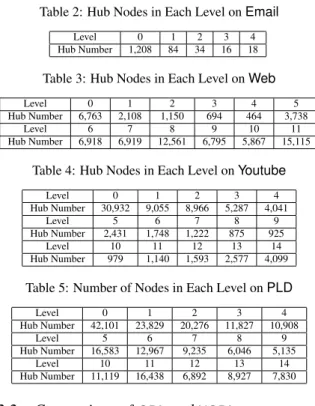
HGPAFor HGPA, we perform the hierarchical partitioning until no edges exist within each subgraph. This is because further parti-tioning cannot gain more improvement. We show the effect of par-titioning levels in Section 6.2.4. We partitionEmailinto 5 levels (yielding25= 32 leaf-level subgraphs),Webinto 12 levels (4,096 leaf-level subgraphs), and bothYoutubeandPLDare partitioned into 15 levels (32,768 leaf-level subgraphs).
The pre-computation space and time cost ofHGPAdepends on the number of hub nodes in each level. We list the number of hub nodes in each level obtained by multi-way hierarchical partitioning of the four datasets in Tables 2–5, where the original graph is at level 0 and the leaf subgraphs are in the maximum level. It can be observed that the number of hub nodes is always much smaller than the total number of nodes in all datasets.
Table 2: Hub Nodes in Each Level onEmail
Level 0 1 2 3 4
Hub Number 1,208 84 34 16 18
Table 3: Hub Nodes in Each Level onWeb
Level 0 1 2 3 4 5
Hub Number 6,763 2,108 1,150 694 464 3,738
Level 6 7 8 9 10 11
Hub Number 6,918 6,919 12,561 6,795 5,867 15,115
Table 4: Hub Nodes in Each Level onYoutube
Level 0 1 2 3 4 Hub Number 30,932 9,055 8,966 5,287 4,041 Level 5 6 7 8 9 Hub Number 2,431 1,748 1,222 875 925 Level 10 11 12 13 14 Hub Number 979 1,140 1,593 2,577 4,099
Table 5: Number of Nodes in Each Level onPLD
Level 0 1 2 3 4 Hub Number 42,101 23,829 20,276 11,827 10,908 Level 5 6 7 8 9 Hub Number 16,583 12,967 9,235 6,046 5,135 Level 10 11 12 13 14 Hub Number 11,119 16,438 6,892 8,927 7,830
6.2.2
Comparison of
GPAand
HGPAThis experiment is to compare the performances ofGPAand HGPAusing default parameters. We report the maximum runtime across all machines as the overall query processing time. For the space cost, we report the maximum space used overall all machines. The pre-computation time is evaluated as the maximum time across all machines. The communication cost is reported as the size of all the data received by the coordinator during the query processing.
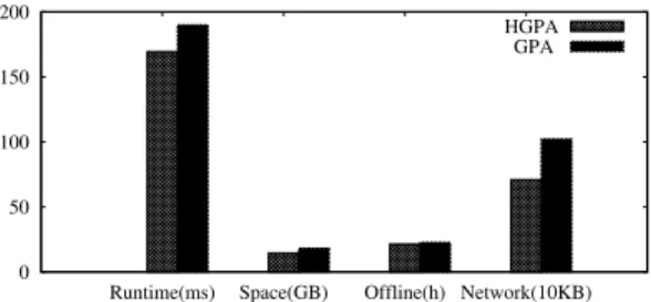
Figure 9 shows the results of the comparison betweenGPAand HGPAonWeb. We observe from the results thatGPAruns a bit slower thanHGPA, becauseHGPAis more load balanced. The maximum space cost and offline pre-computation time ofHGPA are better than that ofGPA, and this is consistent with the theor-etical analysis in Section 4.5. The theortheor-etical communication cost ofHGPAandGPAare the same, while we can observe from the
0 50 100 150 200
Runtime(ms) Space(GB) Offline(h) Network(10KB) HGPA
GPA
Figure 9: Algorithms Comparison onWeb
figure that in practiceHGPAspends less network cost thanGPA. Similar results are observed on the other datasets, and are thus not reported.
SinceHGPAoutperformsGPAin terms of all the aspects con-cerned, we omit the results ofGPAin the subsequent experiments.
6.2.3
Effects of Number of Machines
This experiment is to study the effect of machines number on
HGPA. 100 200 300 400 500 2 4 6 8 10 Runtime (ms) Number of Machines (a) Web 200 400 600 800 1000 2 4 6 8 10 Runtime (ms) Number of Machines (b) Youtube 300 600 900 1200 1500 2 4 6 8 10 Runtime (ms) Number of Machines (c) PLD Figure 10:HGPARuntime
Figures 10(a)–10(c) show the runtime ofHGPAonWeb, You-tube, andPLDwhen we vary the number of machines, respect-ively. We observe that the query processing time drops significantly as the number of machines increases. When we double the number of machines the runtime is nearly reduced by half. The reason is that the computation is evenly distributed to multiple machines in HGPA, and thus the algorithm is highly load-balanced.
10 20 30 40 50 2 4 6 8 10 Space (GB) Number of Machines (a) Web 2 4 6 8 10 12 14 16 18 2 4 6 8 10 Space (GB) Number of Machines (b) Youtube 10 20 30 40 50 60 70 2 4 6 8 10 Space (GB) Number of Machines (c) PLD Figure 11:HGPASpace Cost
Figures 11(a)–11(c) show the space cost of HGPA. Note that each machine only stores the pre-computed vectors of nodes as-signed to it. We report the maximum space cost over all machines. It is observed that the result is as expected, where the maximum space cost is reduced when the number of machines increases. There is no redundant information shared between different machines.
The pre-computation time is shown in Figures 12(a)–12(c). Each machine only needs to do the pre-computation for the nodes stored on it. HGPAis load balanced, and thus the space costs of pre-computation is nearly linear to the number of machines used.
Figures 13(a)–13(c) show the communication cost incurs at query time ofHGPA. We notice even for the largest dataset working on 10 machinesHGPAonly has less than 2MB network cost. It can be observed that the communication cost increases as more machines are employed, which is consistent with our analysis in Theorem 4.
10 25 40 55 70 2 4 6 8 10 Offline Time (h) Number of Machines (a) Web 10 25 40 55 70 85 100 2 4 6 8 10 Offline Time (h) Number of Machines (b) Youtube 20 50 80 110 140 2 4 6 8 10 Offline Time (h) Number of Machines (c) PLD Figure 12:HGPAPre-Computation Time
It is obvious since more machines communicate with the coordin-ator. 600 700 800 900 2 4 6 8 10 Communication Cost(KB) Number of Machines (a) Web 700 800 900 1000 2 4 6 8 10 Communication Cost(KB) Number of Machines (b) Youtube 1200 1250 1300 1350 1400 1450 1500 1550 2 4 6 8 10 Communication Cost(KB) Number of Machines (c) PLD Figure 13:HGPACommunication Cost
6.2.4
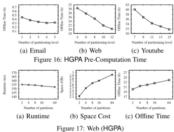
Effect of Partitioning Levels
This set of experiments is to study the effect of the level of the hierarchy of subgraphs on the performance ofHGPA. Figures 14(a)– 14(c) show the runtime for computing PPVs for query nodes on
Email,Web, andYoutube, respectively. Figures 15 and 16 show
the space and time cost of pre-computation on the three datasets. The space and time of pre-computation drop significantly as we increase the number of levels of the graph hierarchy. As the num-ber of levels increases, the numnum-ber of subgraphs in the hierarchy increases exponentially, and thus the size of the subgraphs in leaf-level decreases greatly. However, when in a certain leaf-level there ex-ists few or no edges within each subgraph, further partitioning is unnecessary because it cannot reduce space cost any more. Ac-cording to Equation 7, using more levels needs more computation to construct the PPV, and thus causes slightly longer query pro-cessing time, which can be observed in Figure 14. The communic-ation cost is almost not affected by the number of partition levels, and thus is not reported.
5 6 7 8 9 10 1 2 3 4 5 Runtime (ms)
Number of partitioning level
(a) Email 140 145 150 155 160 165 170 4 6 8 10 12 Runtime (ms)
Number of partitioning level
(b) Web 310 320 330 340 350 360 7 9 11 13 15 Runtime (ms)
Number of partitioning level (c) Youtube Figure 14:HGPARuntime
340 345 350 355 360 1 2 3 4 5 Space (MB)
Number of partitioning level (a) Email 2 3 4 5 6 7 8 4 6 8 10 12 Space (GB)
Number of partitioning level (b) Web 5 5.5 6 6.5 7 7.5 7 9 11 13 15 Space (GB)
Number of partitioning level (c) Youtube Figure 15:HGPASpace Cost
6.2.5
Effect of Multi-way Partitioning
This experiment is to study the effect of the partition strategy. We takeWebas an example in this section, and we observe the similar results on the other datasets. We partitionWebinto 2,4,8,16 and
0.1 0.2 0.3 0.4 0.5 0.6 0.7 1 2 3 4 5 Offline Time (h)
Number of partitioning level
(a) Email 18 20 22 24 26 28 30 32 4 6 8 10 12 Offline Time (h)
Number of partitioning level (b) Web 30 32 34 36 38 40 42 7 9 11 13 15 Offline Time (h)
Number of partitioning level (c) Youtube Figure 16:HGPAPre-Computation Time
140 145 150 155 160 165 170 2 4 8 16 64 Runtime (ms) Number of partitions (a) Runtime 2.2 2.3 2.4 2.5 2.6 2.7 2.8 2.9 3 2 4 8 16 64 Space (GB) Number of partitions (b) Space Cost 17 19 21 23 25 27 2 4 8 16 64 Offline Time (h) Number of partitions (c) Offline Time Figure 17: Web (HGPA)
64 subgraphs in each level and we study the time and space cost for both pre-computation and query processing.
Figure 17(a) shows the query processing time. We observe that the runtime slightly decreases when the number of partitions in each level increases. Figures 17(b) and 17(c) show the space and time cost of the pre-computation. We can see that with more par-titions in each level, the cost of pre-computation increases greatly. We choose the 2-way partitioning strategy by default in this pa-per, as the runtime is close to that of more partitions and its pre-computation space and time cost is the smallest. The partition strategy almost does not affect the communication cost, and thus the we do not report it.
6.2.6
Effect of Tolerance
This experiment is to study the effect of toleranceon the per-formance ofHGPA. For the offline pre-computation, the tolerance decides when the iteration terminates. Again, we takeWebas an example in this section, and we observe similar results on the other datasets. Figures 18(a)–18(d) show the query processing time, the space and time of pre-computation, and the communication cost of HGPAonWeb. We observe that all the four measures increase as we take a smaller tolerance. With a high accuracy, more results of small values are generated, and thus it costs more time for pre-computing the vectors and more space for storing them. At query time, a high accuracy makes the vectors pre-computed have larger size, and thus both PPV construction time and the communication cost increase. 0 50 100 150 200 250 300 350
1e-2 1e-3 1e-4 1e-5 1e-6
Runtime (ms) Tolerance (a) Runtime 0 1 2 3 4 5 6 7
1e-2 1e-3 1e-4 1e-5 1e-6
Space (GB) Tolerance (b) Space Cost 0 10 20 30 40 50 60
1e-2 1e-3 1e-4 1e-5 1e-6
Offline Time (h) Tolerance (c) Offline Time 400 500 600 700 800 900 1000 1100
1e-2 1e-3 1e-4 1e-5 1e-6
Communication Cost(KB)
Tolerance
(d) Communication Cost Figure 18: Web (HGPA)
We also study the exactness ofHGPAwhen we vary the
toler-ance. We take the power iteration method as baseline, treating its PPV result as exact. For each query, we compare the PPV com-puted by HGPAand the power iteration method under the same tolerance. We report the averageL1andL∞of the difference of
two vectors. The results on datasetsEmailandWebare shown in Figures 19(a) and 19(b). It can be observed from the figures that, as
decreases both measures on the differences of two vectors become smaller, which is as expected. The`-norms are nearly in the same order of magnitude with the tolerance. This means we can always obtain a more exact PPV result by setting a smaller tolerance.
L∞ Average L1 1e-6 1e-5 1e-4 1e-3 1e-2
1e-2 1e-3 1e-4 1e-5 1e-6 1e-9 1e-8 1e-7 1e-6 L∞ Average L 1 Error Tolerance (a) Email 1e-6 1e-5 1e-4 1e-3 1e-2
1e-2 1e-3 1e-4 1e-5 1e-6 1e-10 1e-9 1e-8 1e-7 1e-6 L∞ Average L 1 Error Tolerance (b) Web Figure 19:`norm Accuracy
6.2.7
Scalability
Table 6: Graph sizes for scalability study (Meetup) Graph ID # Nodes # Edges
M1 997,304 82,966,338 M2 1,197,009 107,393,088 M3 1,396,054 129,774,158 M4 1,596,455 163,320,390 M5 1,796,226 194,083,414 100 200 300 400 500 M1 M2 M3 M4 M5 Runtime (ms) Graph ID (a) Runtime 4 6 8 10 12 14 16 18 20 M1 M2 M3 M4 M5 Space (GB) Graph ID (b) Space Cost 20 40 60 80 100 M1 M2 M3 M4 M5 Offline Time (h) Graph ID (c) Offline Time Figure 20: Scalability (Meetup)
This experiment is to study the scalability ofHGPAwith the size of graphs. The difficulty is that there does not exist a group of graphs of different sizes but with similar properties. To this end, we build graphs of different sizes by taking different number of meetup events. The sizes of these graphs are listed in Table 6. In this experiment, we fix the number of machines used to be 10 for all graphs.
Figure 20(a) shows the runtime of computing PPVs for query nodes. We observe that the query processing time increases almost linearly with the size of graphs. Figures 20(b) and 20(c) report the space cost and time of pre-computation ofHGPAfor graphs of different sizes. We can see that both the space cost and time increase almost linearly as we increase the size of graphs.
6.2.8
Comparison with General Distributed Graph
Processing Systems
Baseline. To the best of our knowledge, there exists no work for distributed exact PPV computation. Many distributed graph com-putation platforms [47, 48] take the PageRank (PR) problem as a basic graph computing application. In these platforms, the PR problem is usually solved by thepower iterationmethod. Since the personalized PageRank is derived from the PR problem [38],
we can compute PPV by implementing the power iteration method as well on these platforms, which are used as baselines.
We compareHGPAwith the power iteration method implemen-ted on Pregel+ [48] and Blogel [47], which are well-known open-source distributed graph computation platforms (we denote the two algorithms byPregel+andBlogel, respectively). It is shown [48] that Pregel+ outperforms other Pregel systems such as Giraph [19] and GPS [41]. The follow-up work Blogel [47] breaks the bot-tlenecks of vertex-centric models such as Pregel. We compare the runtime and communication cost ofHGPAwithPregel+and
Blogelunder the same tolerance, and the result is shown in
Fig-ures 21(a)– 22(b).
It can be seen that our algorithm is faster thanPregel+and Blo-gelby orders of magnitude onWebandYoutube, andHGPA out-performsPregel+by at least two orders of magnitude in terms of communication cost. We observe that the runtime and communic-ation cost of Pregel+andBlogel increase when the number of machines increases. The reason is as follows:Pregel+is designed based on the general bulk synchronous parallel (BSP) model. It sends massages from vertex to vertex in each iteration of the BSP step, and when the vertices are on different machines it needs a lot of communications between machines. As the number of ma-chines increases, the number of massages increases which costs more communication time. We observe the same phenomenon on
Blogel. However it always outperformsPregel+in terms of the
runtime and communication cost. This is becauseBlogelis based on the block-centric model, and it sends massages from block to block. Our proposed algorithmHGPAsignificantly outperforms the algorithms implemented onPregel+andBlogelfor computing PPVs. As can be observed from the figures, the runtime ofHGPA decreases significantly as the number of machines increases. This is achieved by avoiding the huge communication costs, and thus is more suitable for the online PPV applications.
HGPA Pregel+ Blogel
10 102 103 104 105 2 4 6 8 10 Runtime (ms) Number of Machines (a) Web 102 103 104 105 2 4 6 8 10 Runtime (ms) Number of Machines (b) Youtube Figure 21: Runtime
HGPA Pregel+ Blogel
102 103 104 105 106 2 4 6 8 10 Communication Cost(KB) Number of Machines (a) Web 102 103 104 105 106 2 4 6 8 10 Communication Cost(KB) Number of Machines (b) Youtube Figure 22: Communication Cost
6.2.9
Performance under Centralized Setting
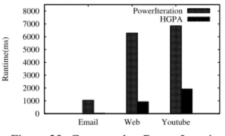
HGPAcan also be implemented on a single machine. We com-pare the runtime ofHGPAin a centralized setting with the power iteration method, under the same error tolerance, and the result is shown in Figure 23. It can be seen that our algorithm is at least 3.5 times faster than the power iteration method. On Email and Web the speedup is much more significant. It demonstrates thatHGPA
0 1000 2000 3000 4000 5000 6000 7000 8000
Email Web Youtube
Runtime(ms)
PowerIteration HGPA
Figure 23: Compared to Power Iteration
can achieve comparable performance in terms of runtime as the al-gorithm proposed in the work [35] on a single machine.
We also compare our work with the state-of-the-art approxim-ate PPV computation methodFastPPV[49]. InFastPPV, the PPV scores less than10−4are discarded. It is shown in [11, 12] that re-moving the small values only sacrifices little accuracy. To compare with the approximate method, we also discard the offline scores that are less than 10−4, and this adapted method is denoted by
HGPA_ad. Since inFastPPVthe number of hub nodes is a
para-meter that affects the trade-off between accuracy and runtime, we compare with this algorithm using different numbers of hub nodes.
0 20 40 60 80 100 120
Fast-100 Fast-1000 HGPA HGPA-ad
(a) Email
1 10 100 1000
Fast-1000 Fast-10000 HGPA HGPA-ad
(b) Web Figure 24: Runtime (ms)
Figure 24 shows the runtime on Email and Web datasets. We use
Fast_hto denote the method ofFastPPVusinghhub nodes. We
notice that our exact methodHGPAis faster thanFastPPVon small dataset and slower thanFastPPVon the large one. By discarding tiny PPV scores, we notice that the adapted methodHGPA_adruns faster thanFastPPVby orders of magnitude on both datasets. Note that in this set of experiments our algorithm is implemented on a single machine. On the distributed computing platforms, our al-gorithm will be much faster.
We next evaluate the accuracy of the four algorithms and use the result computed by power iteration as exact. We use averageL1
andL∞as we used in Section 6.2.6. Figure 25 show the`norm
accuracy comparison on Email and Web datasets. On all meas-ures, it is not surprised to observe thatHGPAis much better than
FastPPVsince the computing model of our algorithm is exact. We
notice that our approximate HGPA_adalso consistently outper-formsFastPPVin terms of accuracy.
10-8 10-6 10-4 10-2 100 AverageL1 Linf Fast-100 Fast-1000 HGPA HGPA-ad (a) Email 10-8 10-6 10-4 10-2 100 AverageL1 Linf Fast-1000 Fast-10000 HGPA HGPA-ad (b) Web Figure 25:`norm Accuracy
In summary, our proposed distributed algorithmsGPAandHGPA have low communication cost and are load-balanced with
accept-able pre-computation and space cost. HGPAconsistently outper-formsGPA, and it outperforms the power iteration method imple-mented on general graph processing platforms such as Pregel+ and Blogel by orders of magnitude. In the centralized setting,HGPA can achieve comparable query time with the exact method [35] and the approximate method [49]. Its adapted versionHGPA_adis able to outperform the approximate method [49] in terms of both efficiency and accuracy.
6.2.10
Exact vs Approximate
This experiment extends the study of Section 6.2.9 to show the advantage of exact PPVs compared to approximate PPVs. We use two accuracy metrics, i.e., Precision andKendall’sτ(by following the work [11, 49]), to compare the top-100 nodes obtained from each algorithm with the result of the power iteration method. In a nutshell, Precision is based on the value of top-k PPV results, and Kendall is based on the percentage of the correct node pair order. The detailed definition can be referred to [11]. Figure 26 shows the results onEmailandWeb. We observe that on both metricsHGPAperforms much better than FastPPV [49], and even the adaptive algorithmHGPA_adachieves nearly full score. This indicates that about 30% of the top-100 nodes returned by FastPPV are wrong, and about 10% node pairs are ordered incorrectly.
0.6 0.7 0.8 0.9 1
Precision RAG Kendall
Accuracy Fast-100 Fast-1000 HGPA HGPA-ad (a) Email 0.6 0.7 0.8 0.9 1
Precision RAG Kendall
Accuracy Fast-1000 Fast-10000 HGPA HGPA-ad (b) Web Figure 26: Accuracy
7.
RELATED WORK
The personalized PageRank(PPR) has been widely used in vari-ous fields of applications, such as community detection [3,21], link prediction [4], and recommendation systems [22, 27].
Exact PPV computation.PPR was first proposed by Jeh and
Wi-dom [25]. It usually needs to be computedin an online manner,
and thus has a high requirement for efficiency. A straightforward
way of computing the Personalized PageRank Vector for a given set of nodes is the power iteration method, which is prohibitively expensive in time and is not suitable even for offline scenarios.
Due to the hardness of computing the exact PPV, Jeh and Widom propose to limit the preference nodes in a subset of a specified hub node set [25]. Therefore, this approach cannot be used to compute the exact PPV for arbitrary preference node set. We will introduce more about the algorithm in Section 2.
Maehara et al. [35] propose an iteration-based method that com-putes exact PPVs by exploiting graph structures. They decompose a graph into a core and a small tree-width graph. The two compon-ents are processed differently, and the PPV is constructed using the processed results. Unfortunately, this approach is not able to com-pute exact PPVs in a distributed manner. According to the experi-mental study, this method is about five times faster than the power iteration method. As shown in the experimental study, our distrib-uted algorithmHGPAis faster than the power iteration method im-plemented on general graph processing engines by orders of mag-nitude.
Approximate methods for PPV.Most of existing studies
com-pute PPVs approximately to trade for efficiency. Some proposals (e.g., [6, 14]) utilize the Monte Carlo simulation methods, while
some other studies (e.g., [44]) utilize the matrix factorization. Zhu et al. [49] propose an approximate method based on the concept of the inverse P-distance [25]. They first partition the tours into different tour sets according to their importance. Then, they design an algorithm to aggregate the contribution of tours from the most important ones to less important ones. In the experimental study, we show that our exact algorithmHGPAis able to achieve similar query time to the approximate algorithm [49] while obtaining much better accuracy, and an adapted version ofHGPAoutperforms the approximate algorithm [49] in terms of both efficiency and accur-acy.
Top-k and node-to-node search for PPV.Some approaches [16–
18,46] aim to find a small part of the PPV. That is, for a query node, they only identify its top-krelevant nodes and omit the other nodes. Lofgren et al. [31, 32] study how to estimate the node-to-node PPV score. Given a query nodeu, a target nodevand thresholdδ, they estimate whetherru(v) > δis true. All these methods cannot be used for computing the whole PPV w.r.t. a given query node set. However, finding top-k or estimating node-to-node PPV value is insufficient for many applications (e.g., [4,8,11]) which require the PPV scores of all nodes.
Distributed PPV computation. There also exist studies on
dis-tributed computation of approximate PPVs. In particular, Bahmani et al. [5] proposes a distributed algorithm based on MapReduce utilizing Monte Carlo simulation, which has no guaranteed error bound. The general graph processing engines, such as Pregel [36], Pregel+ [48] and Blogel [47], can be used for various distributed graph processing. As shown in the work [36], the power iteration method can be implemented on Pregel to compute PageRank, and thus PPVs. However, using these engines always induces multiple rounds of communications between machines; therefore, the com-munication cost is large and the query processing is slow, which make them impractical for applications of PPVs that have a high re-quirement on efficiency. In contrast, our proposed algorithms only require the communication between the machines and the coordin-ator once at query time. As shown in the experimental study, our algorithm significantly outperforms the PPV computation based on Pregel+ [48] and Blogel [47].
8.
CONCLUSION
In this paper, we propose novel and efficient distributed algorithms that are able to compute the exact PPV for all nodes. The pro-posed algorithms can be implemented on a general coordinator-based share-nothing distributed computing platform. The processors only need to communicate with the coordinator once at query time in our algorithms. We first develop the algorithmGPAthat works based on subgraphs. To further improve the performance, we pro-poseHGPAbased on a hierarchy of subgraphs, which has smaller space cost and better load balance and efficiency thanGPA. The experimental study shows thatHGPAhas excellent performance in terms of efficiency, space cost, communication cost, and scalabil-ity. Our algorithmHGPAoutperforms the PPV computation using power iteration based on two distributed graph processing systems by orders of magnitude. Further, an adapted version ofHGPA out-performs the state-of-the-art approximate algorithm [49] in terms of both efficiency and accuracy. In the future we would like to fur-ther study how to reduce the number of hub nodes.
9.
ACKNOWLEDGMENT
This work was carried out at the Rapid-Rich Object Search(ROSE) Lab at the Nanyang Technological University, Singapore. The ROSE Lab is supported by the National Research Foundation, Singapore, under its Interactive Digital Media(IDM) Strategic Research Pro-gramme.
10.
REFERENCES
[1] K. Andreev and H. Racke. Balanced graph partitioning.
Theory of Computing Systems, 39(6):929–939, 2006.
[2] I. Antonellis, H. G. Molina, and C. C. Chang. Simrank++: Query rewriting through link analysis of the click graph.
PVLDB, 1(1):408–421, 2008.
[3] H. Avron and L. Horesh. Community detection using time-dependent personalized pagerank. InICML, pages 1795–1803, 2015.
[4] L. Backstrom and J. Leskovec. Supervised random walks: predicting and recommending links in social networks. In WSDM, pages 635–644, 2011.
[5] B. Bahmani, K. Chakrabarti, and D. Xin. Fast personalized pagerank on mapreduce. InKDD, pages 973–984, 2011. [6] B. Bahmani, A. Chowdhury, and A. Goel. Fast incremental
and personalized pagerank.PVLDB, 4(3):173–184, 2010. [7] B. Bahmani, R. Kumar, M. Mahdian, and E. Upfal. Pagerank
on an evolving graph. InProceedings of the 18th ACM SIGKDD international conference on Knowledge discovery
and data mining, pages 24–32. ACM, 2012.
[8] A. Balmin, V. Hristidis, and Y. Papakonstantinou.
Objectrank: Authority-based keyword search in databases. In VLDB, pages 564–575, 2004.
[9] P. Berkhin. Bookmark-coloring algorithm for personalized pagerank computing.Internet Mathematics, 3(1):41–62, 2006.
[10] T. N. Bui and C. Jones. Finding good approximate vertex and edge partitions is np-hard.Information Processing Letters, 42(3):153–159, 1992.
[11] S. Chakrabarti. Dynamic personalized pagerank in entity-relation graphs. InWWW, pages 571–580, 2007. [12] S. Chakrabarti, A. Pathak, and M. Gupta. Index design and
query processing for graph conductance search.The VLDB
Journal, 20(3):445–470, 2011.
[13] U. Feige and R. Krauthgamer. A polylogarithmic
approximation of the minimum bisection.SIAM Journal on
Computing, 31(4):1090–1118, 2002.
[14] D. Fogaras, B. Rácz, K. Csalogány, and T. Sarlós. Towards scaling fully personalized pagerank: Algorithms, lower bounds, and experiments.Internet Mathematics, 2(3):333–358, 2005.
[15] S. Fortunato. Community detection in graphs.Physics
reports, 486(3):75–174, 2010.
[16] Y. Fujiwara, M. Nakatsuji, M. Onizuka, and M. Kitsuregawa. Fast and exact top-k search for random walk with restart.
PVLDB, 5(5):442–453, 2012.
[17] Y. Fujiwara, M. Nakatsuji, H. Shiokawa, T. Mishima, and M. Onizuka. Efficient ad-hoc search for personalized pagerank. InICDM, pages 445–456, 2013.
[18] Y. Fujiwara, M. Nakatsuji, T. Yamamuro, H. Shiokawa, and M. Onizuka. Efficient personalized pagerank with accuracy assurance. InKDD, pages 15–23, 2012.
[19] A. Giraph. http://giraph.apache.org/.
[20] D. Gleich, L. Zhukov, and P. Berkhin. Fast parallel pagerank: A linear system approach.Yahoo! Research Technical Report YRL-2004-038, available via http://research. yahoo.
com/publication/YRL-2004-038. pdf, 13:22, 2004.
[21] D. F. Gleich and C. Seshadhri. Vertex neighborhoods, low conductance cuts, and good seeds for local community methods. InKDD, pages 597–605, 2012.
[22] P. Gupta, A. Goel, J. Lin, A. Sharma, D. Wang, and
R. Zadeh. WTF: the who to follow service at twitter. In WWW, pages 505–514, 2013.
[23] B. Hendrickson and T. G. Kolda. Graph partitioning models for parallel computing.Parallel Computing,
26(12):1519–1534, 2000.
[24] G. Jeh and J. Widom. Simrank: a meas
![Figure 2: Example of graph partition and hub nodes Recall that the PPV construction of the method [25] is based on Equation 4](https://thumb-us.123doks.com/thumbv2/123dok_us/933974.2621098/4.918.159.362.230.348/figure-example-graph-partition-recall-construction-method-equation.webp)