A Simulation Model for Transport in a Grid-based Manufacturing System
Leo van Moergestel, Erik Puik, Dani¨el Telgen,
Mathijs Kuijl, Bas Alblas and Jaap Koelewijn
Department of Computer science HU Utrecht University of Applied Sciences
Utrecht, the Netherlands Email: [email protected]
John-Jules Meyer
Intelligent systems groupUtrecht University Utrecht, the Netherlands Email: [email protected]
Abstract—Standard mass-production is a well-known manufac-turing concept. To make small quantities or even single items of a product according to user specifications at an affordable price, alternative agile production paradigms should be investigated and developed. The system presented in this paper is based on a grid of cheap reconfigurable production units, called equiplets. A grid of these equiplets is capable to produce a variety of different products in parallel at an affordable price. The underlying agent-based software for this system is responsible for the agile manufacturing. An important aspect of this type of manufacturing is the transport of the products along the available equiplets. This transport of the products from equiplet to equiplet is quite different from standard production. Every product can have its own unique path along the equiplets. In this paper several topologies are discussed and investigated. Also, the planning and scheduling in relation to the transport constraints is subject of this study. Some possibilities of realization are discussed and simulations are used to generate results with the focus on efficiency and usability for different topologies and layouts of the grid and its internal transport system.
Keywords-Multiagent-based manufacturing; Flexible transport.
I. INTRODUCTION
In standard batch processing the movement of products is mostly based on a pipeline. Though batch processing is a very good solution for high volume production, it is not apt for agile manufacturing when different products at small quantities are to be produced by the production equipment. Grid manufacturing will first be explained, followed by a section about transport in the grid. After introducing the software tools built, the results are presented and discussed. Finally, related work and a conclusion will be presented.
II. GRID MANUFACTURING
In grid production, manufacturing machines are placed in a grid topology. Every manufacturing machine offers one or more production steps and by combining a certain set of production steps, a product can be made. This means that when a product requires a given set of production steps and the grid has these steps available, the product can be made [1]. The software infrastructure that has been used in our grid, is agent-based. Agent technology opens the possibilities to let this grid operate and manufacture different kinds of products
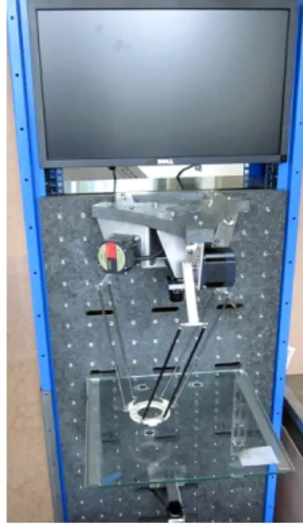
in parallel, provided that the required production steps are available [2]. The manufacturing machines that have been built in our research group are cheap and versatile. These machines are called equiplets and consist of a standardized frame and subsystem on which several different front-ends can be attached. The type of front-end specifies what production steps a certain equiplet can provide. This way every equiplet acts as a reconfigurable manufacturing system (RMS) [3]. A picture of an equiplet with a delta-robot front-end is shown in Figure 1. This equiplet is capable of pick and place actions. A computer vision system is part of the frontend. This way the equiplet can localise parts and check the final position they are put in. For a product to be made a sequence of production
Figure 1: An equiplet with a delta-robot frontend.
steps has to be done. More complex products need a tree of sequences, where every sequence ends in a half-product or part, needed for the end product. The equiplet is represented in software by a so-called equiplet agent. This agent advertises its capabilities as production steps to a blackboard that is available in a multiagent system where also so-called product agents live. A product agent is responsible for the manufacturing of a single product and knows what to do, the equiplet agents knows how to do it. A product agent selects a set of equiplets based on the production steps it needs and tries to match these
steps with the steps advertised by the equiplets. The planning and scheduling of a product is an atomic action, done by the product agent in cooperation with the equiplet agent and takes seven steps [4]. Let us first assume that a single sequence of steps is needed.
1) From the list of production steps, build a set of equiplets offering these steps;
2) Ask equiplets about the feasibility and duration of the steps;
3) Indicate situations where consecutive steps on the same equiplet are possible;
4) Generate at most four paths along equiplets; 5) Calculate the paths along these equiplets;
6) Schedule the shortest product path using first-fit (take the first opportunity in time for a production step) and a scheduling scheme known as earliest deadline first (EDF) [4];
7) If the schedule fails, try the next shortest path; For more complex products, consisting of a tree of sequences, the product agent spawns child agents, that are each respon-sible for a sequence. The parent agent is in control of its children and acts as a supervisor. It is also responsible for the last single sequence of the product. In Figure 2, the first two halfproducts are made using stepsequences < σ1, σ2 > and
< σ3, σ4>. These sequences are taken care of by child agents,
while the parent agent will complete the product by performing the step sequence < σ4, σ7, σ2, σ1 >. Every product agent is
1 2
3 4
4 7 2 1
Figure 2: Manufacturing of a product consisting of two half-products
responsible for only one product to be made. The requests for products arrive at random. In the implementation we have made, a webinterface helps the end-user to design his specific product. At the moment all features are selected a product agent will be created. During manufacturing a product is guided by the product agent from equiplet to equiplet. This will in general be a random walk along the equiplets. This random walk is more efficient when the equiplets are in a grid arrangement against a line arrangement as used in batch processing.
III. TRANSPORT IN THE GRID
In the production grid, there is at least the stream of prod-ucts to be made. Another stream might be the stream of raw material, components or half-products used as components. We will refer to this stream as the stream of components. These components could be stored inside the equiplets, but in that case there is still a stream of supply needed in case the locally stored components run short. This increases the logistic complexity of the grid model. In the next subsections, models will be introduced that alleviate the complexity by combining the stream of products with the stream of components. A. Buiding box model
In the building box model, a tray is loaded with all the components to create the product. To maintain agility, this
set of components can be different for every single product. Before entering the grid, the tray is filled by passing through a pipeline with devices providing the components. In this phase a building box is created that will be used by the grid to assemble the product. The equiplets in the grid are only used for assembling purposes. Figure 3 shows the setup.
Part-supply Line
Manufacturing Grid
Figure 3: Production system with supply pipeline
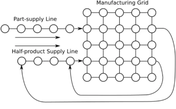
A problem with the previous setup is the fact that more complex products should be built by combining subparts that should be constructed first. In the previously presented setup all parts needed for the construction of the subparts should be collected in the building box, making the assembling process more complicated. Another disadvantage of putting all components for all subparts together in a building box is that this slows down the production time, because normally subparts can be made in parallel. A solution is shown in the setup of Figure 4. Subparts can be made in parallel and are input to the supply-line that eventually could be combined with the original supply-line. The next refinement of the system is
Part-supply Line
Manufacturing Grid
Half-product Supply Line
Figure 4: Production system with loops
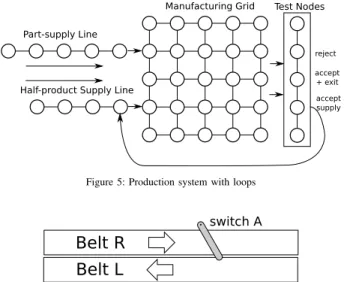
presented in Figure 5. Here a set of special testnodes has been added to the system. These nodes are actually also equiplets, but these equiplets have a front-end that makes them suited for testing and inspecting final products as well as subparts that should be used for more complicated products. A test can also result in a reject and this will also inform the product agent about the failure. If the product agent is a child agent constructing a subpart, it should consult the parent agent if a retry should be done. In case it is the product agent for the final product, it should ask its maker what to do.
B. Conveyor belt-based systems
A conveyor belt is a common device to transport material. Several types are in use in the industry. Without going into detail, some kind of classification will be presented here:
Part-supply Line
Manufacturing Grid
Half-product Supply Line
Test Nodes accept supply accept + exit reject
Figure 5: Production system with loops
Belt R
Belt L
switch A
switch B
Figure 6: Bidirectional conveyor belt with switches
• belts for continuous transport in one direction;
• belts with stepwise transport from station to station. These types of belts can be used in batch environ-ments, where every step takes the same amount of time and the object should be at rest when a production step is executed;
• belts with transport is two directions. This can also be realised by using two one direction belts, working in opposite direction.
In Bussmann [5], an agent-based production system is built us-ing transport belts in two directions where a switch mechanism can move a product from one belt to another. A special switch-agent is controlling the switches and thus controlling the flow of a product along the production machines. In Figure 6 this solution is shown. Switch A is activated and will shift products from belt R to the belt L that will move it to the left. This concept fits well in the system developed by Bussmann, because that system is actually a batch-oriented system. In a grid the use of conveyor belts might be considered, but for agile transport several problems arise, giving rise to complicated solutions:
• should the direction in the grid consist of one-way paths or should be chosen for bidirectional transport?
• a product should be removed from the moving belt during the execution of a production step. A stepwise transport is inadequate, because of the fact that pro-duction steps can have different execution times in our agile model. This removal could be done by a switch mechanism as used by Bussmann, but every equiplet should also have it own switch-unit to move the product back to the belt.
• because the grid does not have a line structure for reasons explained in the first part of this chapter, a lot of crossings should be implemented. These crossings can also be realised with conveyor belt techniques, but it will make the transport system as a whole expensive and perhaps more error-prone.
C. Autonomous transport
An alternative for conveyor belts is the use of automatic guided vehicles (AGV). An AGV is a mobile robot that follows certain given routes on the floor or uses vision, ultrasonic sonar or lasers to navigate. These AGVs are already used in industry mostly for transport, but they are also used as moving assembly platforms. This last application is just what is needed in the agile manufacturing grid. The AGV solution used to be expensive compared to conveyor belts but some remarks should be made about that:
• These AGV offer a very flexible way for transport that fits better in non-pipeline situations;
• Low cost AGV platforms are now available;
• From the product agent view, an AGV is like an equiplet, offering the possibility to move from A to B.
• A conveyor-belt solution that fits the requirements needed in grid productions will turn out to be a com-plicated and expensive system due to the requirements for flexible transport.
In the grid a set of these AGVs will transport the product between equiplets and will be directed to the next destination by product agents.
1) AGV system components: An AGV itself is a driverless mobile robot platform or vehicle. This AGV is mostly a battery-powered system. To use an AGV, a travel path should be available. When more then one AGV is used on the travel path. A control system should manage the traffic and prevent collisions between the AGVs or prevent deadlock situations. The control system can be centralised or decentralised.
2) AGV navigation: There are plenty ways in which nav-igation of AGVs has been implemented. The first division in techniques can be made, based on whether the travel path itself is specially prepared to be used by AGVs. This can be done by:
• putting wires in the path the AGV can sense and follow;
• using magnetic tape to guide the AGV;
• using coloured paths, by using adhesive tape on the path to direct the AGV;
• using transponders, so the AGV can localise itself. The second type of AGV does not require a specially prepared path. In that case navigation is done by using:
• laser range-finders
• ultrasonic distance sensors
• vision systems
Though it might look as if the decision for using AGVs has already been made, further research should be done to see what the efficiency will be for several implementations. This will be the subject of the next two sections.
IV. SOFTWARE TOOLS
Two simulation software packages have been built. A simulation of the scheduling for production and a simulation for the path planning. The path planning tool will be used to calculate the efficiency for different transport interconnections. The scheduling tool will be used to calculate the number of active product agents within the grid. This number is important, because it will tell how many products should be temporally stored, waiting for the next production step to be executed.
A. Path planning simulation software
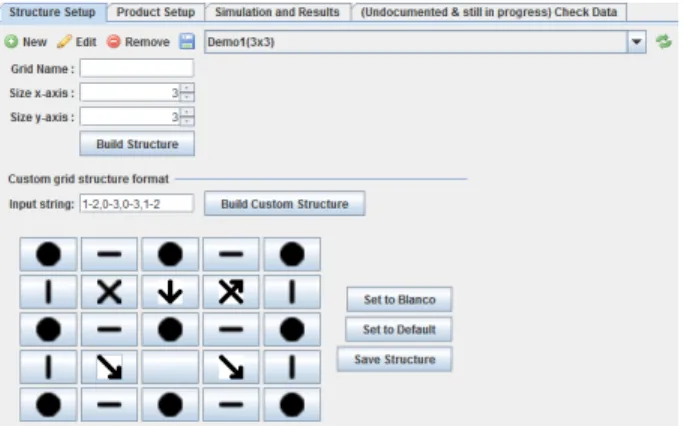
A path planning tool has been built, to calculate a path a certain product has to follow along the equiplets. The Dijkstra path algorithm has been used [6]. The tool can work on different grid transport patterns. This tool will be used to study several possible grid topologies. A screen-shot of the graphical user interface of the tool is shown in Figure 7. Several different topologies and interconnections can be chosen by clicking the appropriate fields in the GUI. The average transport path for all nodes is one of the results of this simulation.
Figure 7: Path planning GUI
B. Scheduling simulation software
The software for the scheduling simulations consists of two parts. One part is a command-line tool that is driven by a production scenario of a collection of product agents, each having their own release time, deadline and set of production steps. This production scenario is a human readable XML-file. The second part is a GUI for visualisation of the scheduling system. In Figure 8 a screen shot of this visualisation tool is shown.
Figure 8: GUI of the scheduling simulator
Figure 9: Standard fully connected grid
Figure 10: grid with bidirectional lanes and bidirectiona backbone lanes
V. RESULTS
To calculate the average pathlength in the grid for different paths, several structures have been investigated. Some of these structures were chosen to fit conveyor belt solutions of some type. All structures will also fit within the AGV-based solution.
• A fully connected grid. where all paths are bidirec-tional paths as in Figure 9.
• A grid where all paths are bidirectional, but this design has removed the crossings as in Figure 10. This structure could be implemented by conveyor belts in combination with switches;
• A structure with five unidirectional paths and two bidirectional paths as in Figure 11. This structure is also a possible implementation with conveyor belts;
• A structure with bidirectional paths combined in a single backbone as in Figure 12;
• A structure with five bidirectional paths and two unidirectional paths as in Figure 13;
• A fully connected grid, but now with half of the paths unidirectional as in Figure 14.
For all these structures the average path is the result from a simulation of 1000 product agents, all having a random walk within the grid. Each product agent has an also random set of equiplets it has to visit ranging from 2 to 50 equiplets per product agent. Every path or hop between adjacent nodes is considered to be one unit length. If the paths have no crossings, a conveyor belt might be used, because crossing belts will result in a more complex system. All structures can also be implemented with AGVs. For some structures the average path can also easily be calculated and the results of these exact calculations are within 1% of the simulation results.
Figure 11: Grid with unidirectional lanes and bidirectional backbone lanes
Figure 12: E-shaped connection, with bidirectional lanes
Figure 13: Bidirectional lanes with unidirectional backbones
Figure 14: Fully connected grid with unidirectional lanes
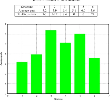
The results of the simulation are given in a table and also plotted as a histogram in Figure15. In Table I, a second outcome from the simulation is also shown. This is the percentage of agents that could find an alternative path of the same length. This result is of interest when in a traffic control implementation, alternative paths become important.
As could be expected, the best result is achieved in the fully connected grid with bidirectional paths. Changing the grid to
TABLE I: Results of the simulatiom
Structure 1 2 3 4 5 6 Average path 3.2 3.9 6.4 5.1 6.0 3.6 % Alternatives 60 16.7 8.4 0 0 27 0 1 2 3 4 5 6 7 0 1 2 3 4 5 6 7 Average path Structure
Figure 15: Simulation results for different structures
an almost identical structure of Figure 14 with unidirectional paths, results in only a small penalty. This structure could also be useful in an AGV-based transport system, reducing collision problems because of the one-way paths used. Both structures also offer a relative high percentage of alternative paths, that could also be useful in an AGV-based system. The structures that fit a conveyor belt solution show a path length that is considerably higher.
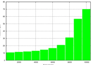
The next results were generated using the scheduling tool. This tool was used in earlier research [4] to discover the scheduling approach to be used. Earliest deadline first (EDF) turned out to be a good choice. In Figure 16 the average number of product agents in a manufacturing grid consisting of 10 equiplets is shown for different sizes of test sets. Every product agent has a random number of equiplets to visit ranging from 1 to 20. Also, the time window between release time and deadline is random between 1 to 20 times the total production time of a product. The number of timesteps is 10000 and the duration of a production step is 1 timestep. For a set with 10000 product agents, the grid is actually overloaded as can be seen in Figure 17, where the number of scheduling failures is over 1000. Another simulation shows the same effect. This simulation is based on one scenario with a linear increasing amount of product agents in time as shown in Figure 18. In this graph, a product is considered active in the grid between its release time and its deadline. The actual number of products in the grid is shown in Figure 19. When we look at the actual number of active products in the grid, the resulting graph shows an remarkable shape. In the beginning, the actual number is even less than the number plotted in the graph of Figure 18. This is due to the fact that in a grid that is only used by a small amount of products, every product will be finished far before its deadline. A finished product is not considered active in the grid any more. However, at a certain point there is a steep increase in the number of products and the graph saturates at the same level of 70 products as
0 10 20 30 40 50 60 70 80 2000 4000 6000 8000 10000 Products in grid
Test set size
Figure 16: Simulation Results for different sizes op product sets
0 200 400 600 800 1000 2000 4000 6000 8000 10000 Failures
Test set size
Figure 17: Simulation Results for different sizes op product sets
0 50 100 150 200 250 0 1000 2000 3000 4000 5000 6000 7000 8000 9000 10000 number of products timesteps
number of product-agents in grid
Figure 18: Increasing number of active products in the grid
shown in Figure 16 for a test set of 10000. The number of rejected products due to a failing scheduling will increase. This also means that overloading the grid will generate many
0 10 20 30 40 50 60 70 80 90 0 1000 2000 3000 4000 5000 6000 7000 8000 9000 10000 number of produ cts timesteps
actual number of products in grid
Figure 19: Number of products in the grid
active products that should be stored somewhere, because in this given situation, only 10 products can be handled by an equiplet.
VI. DISCUSSION
For the agile grid-based and agent-based manufacturing the buildingbox as well as the AGV-based system offer advantages:
• By using a building box, the transport of parts to the assembling machines (equiplets) is combined with the transport of the product to be made. It will not happen that a part is not available during manufacturing;
• Because the product as well as it parts use one particular AGV during the production, there is never a competition for AGV during the manufacturing process;
• An AGV can use the full possibility and advantage of the grid-based system being a compact design resulting in short average paths;
• The product agent knows which equiplets it should visit and thus can use the AGV in the same way as an equiplet. The product agent can instruct the AGV agent to bring it to the next equiplet in the same way as it can instruct an equiplet agent to perform a production step;
• An AGV can bring the production platform exact to the right position for the equiplet and can even add extra movement in the X-Y plane or make a rotation around the Z-axis;
• If an AGV fails during production the problem can be isolated and other AGVs can continue to work. In a conveyor belt system a failing conveyor might block the whole production process.
There are also some disadvantages
• There should be a provision for charging the battery of the AGV.
• Simulations show that the amount of agents in the grid shows a strong increase in a grid that is loaded over 80%. This will result in a lot of AGVs in the grid leading to traffic jam;
• Only products that fit within the building box manu-facturing model can be made.
VII. RELATED WORK
Using agent technology in industrial production is not new though still not widely accepted. Important work in this field has already been done. Paolucci and Sacile [7] give an extensive overview of what has been done in this field. Their work focuses on simulation as well as production scheduling and control [8]. The main purpose to use agents in [7] is agile production and making complex production tasks possible by using a multi-agent system. Agents are also introduced to deliver a flexible and scalable alternative for manufacturing execution systems (MES) for small production companies. The roles of the agents in this overview are quite diverse. In simulations agents play the role of active entities in the production. In production scheduling and control agents support or replace human operators. Agent technology is used in parts or subsystems of the manufacturing process. We on the contrary based the manufacturing process as a whole on agent technology. In our case a co-design of hardware and software was the basis.
Bussmann and Jennings [5][9] used an approach that com-pares to our approach. The system they describe introduced three types of agents, a workpiece agent, a machine agent and a switch agent. Some characteristics of their solutions are:
• The production system is a production line that is built for a certain product. This design is based on redundant production machinery and focuses on production availability and a minimum of downtime in the production process. Our system is a grid and is capable to produce many different products in parallel;
• The roles of the agents in this approach are different from our approach. The workpiece agent sends an invitation to bid for its current task to all machine agents. The machine agents issue bids to the work-piece agent. The workwork-piece agent chooses the best bid or tries again. In our system the negotiating is between the product agents, thus not disrupting the machine agents;
• They use a special infrastructure for the logistic sub-system, controlled by so called switch agents. Even though the practical implementation is akin to their solution, in our solution the service offered by the logistic subsystems can be considered as production steps offered by an equiplet and should be based on a more flexible transport mechanism.
So there are however important differences to our approach. The solution presented by Bussmann and Jenning has the characteristics of a production pipeline and is very useful as such, however it is not meant to be an agile multi-parallel production system as presented here.
Other authors focus on using agent technology as a solution to a specific problem in a production environment. The work
of Xiang and Lee [10] presents a scheduling multiagent-based solution using swarm intelligence. This work uses negotiating between job-agents and machine-agents for equal distribution of tasks among machines. The implementation and a simu-lation of the performance is discussed. In our approach the negotiating is between product agents and load balancing is possible by encouraging product agents to use equiplets with a low load. We did not focus on a specific part of the production but we developed a complete production paradigm based on agent technology in combination with a production grid. This model is based on two types of agents and focuses on agile multiparallel production. There is a much stronger role of the product agent and a product log is produced per product. This product agent can also play an important role in the life-cycle of the product. The design and implementation of the production platforms and the idea to build a production grid can be found in Puik[1].
VIII. CONCLUSION
Agent-based grid manufacturing is a feasible solution for agile manufacturing. Some important aspects of this manufac-turing paradigm have been discussed here. Transport can be AGV-based provided that the load of the grid should be kept under 80% to overcome the temporary storage requirements.
REFERENCES
[1] E. Puik and L. v. Moergestel, “Agile multi-parallel micro manufacturing using a grid of equiplets,” Proceedings of the International Precision Assembly Seminar (IPAS 2010), 2010, pp. 271–282.
[2] L. v. Moergestel, J.-J. Meyer, E. Puik, and D. Telgen, “Decentralized autonomous-agent-based infrastructure for agile multiparallel manufac-turing,” Proceedings of the International Symposium on Autonomous Distributed Systems (ISADS 2011) Kobe, Japan, 2011, pp. 281–288.
[3] Z. M. Bi, S. Y. T. Lang, W. Shen, and L. Wang, “Reconfigurable
manufacturing systems: the state of the art,” International Journal of Production Research, vol. 46, no. 4, 2008, pp. 599–620.
[4] L. v. Moergestel, J.-J. Meyer, E. Puik, and D. Telgen, “Production scheduling in an agile agent-based production grid,” Proceedings of the Intelligent Agent Technology (IAT 2012), 2012, pp. 293–298. [5] S. Bussmann, N. Jennings, and M. Wooldridge, Multiagent Systems for
Manufacturing Control. Berlin Heidelberg: Springer-Verlag, 2004. [6] M. Sniedovich, “Dijkstras algorithm revisited: the dynamic
program-ming connexion,” Control and Cybernetics, vol. 35, no. 3, 2006, pp. 599–620.
[7] M. Paolucci and R. Sacile, Agent-based manufacturing and control
systems : new agile manufacturing solutions for achieving peak
per-formance. Boca Raton, Fla.: CRC Press, 2005.
[8] E. Montaldo, R. Sacile, M. Coccoli, M. Paolucci, and A. Boccalatte, “Agent-based enhanced workflow in manufacturing information sys-tems: the makeit approach,” J. Computing Inf. Technol., vol. 10, no. 4, 2002, pp. 303–316.
[9] N. Jennings and S. Bussmann, “Agent-based control system,” IEEE
Control Systems Magazine, vol. 23, no. 3, 2003, pp. 61–74. [10] W. Xiang and H. Lee, “Ant colony intelligence in multi-agent dynamic
manafacturing scheduling,” Engineering Applications of Artificial In-telligence, vol. 16, no. 4, 2008, pp. 335–348.