Rent Control and Misallocation
by
Gintautas Bloze
and
Morten Skak
Discussion Papers on Business and Economics
No. 7/2009
FURTHER INFORMATION Department of Business and Economics Faculty of Social Sciences University of Southern Denmark Campusvej 55 DK-5230 Odense M Denmark Tel.: +45 6550 3271 Fax: +45 6550 3237 E-mail: [email protected] ISBN 978-87-91657-35-1 http://www.sdu.dk/osbec
September 2009
Rent Control and Misallocation
by
Gintautas Bloze* and Morten Skak* University of Southern Denmark**
Abstract
The paper considers welfare effects of rent control when it is applied only in a sector of a rental housing market. In rent controlled sectors of the Danish rental housing market, we find welfare reducing overallocation of square meters between 9 and 17 per cent of actual
allocations. Looking at the 20 per cent most overallocated households, the overallocation of square meters is between 42 and 92 per cent, and the estimated corresponding welfare loss ranges from 1.5 to 5.3 per cent of the average annual rent in the sectors.
JEL Classification: D11, D61, L51, R21, R31
Keywords: Rent control, Housing, Regulation, Price ceiling, Rationing, Allocation
* Department of Business and Economics, Campusvej 55, DK-5230 Odense M, Denmark. Corresponding author Morten Skak: Phone +45 6550 2116. E-mail [email protected].
** We thank Yew-Kwang Ng for fruitful discussions. Errors and omissions remain our responsibility alone. The paper is written as a part of the Centre for Housing and Welfare - Realdania Research project. Economic support from Realdania is acknowledged.
1. Introduction
In their paper The Misallocation of Housing under Rent Control, Glaeser and Luttmer (1997 and 2003) point out that rent control on a perfectly competitive housing market incurs not only the well-known welfare loss from reduced supply, but also a welfare loss from
misallocation among households of rent controlled dwellings. This result is demonstrated in a partial equilibrium model of a rental housing market with universal rent control. However, rent control is often implemented in a sector of the rental housing market with free rent setting in other sectors. Thus, the Los Angeles rent control law of 1978 exempted newly constructed units, see Fallis and Smith (1984), and rent control in Vancouver, British Colombia, exempted units built after 1974, see Marks (1984). In the New York case studied by Glaeser and
Luttmer (2003) “rent-control regulations by and large exclude apartments in buildings with fewer than five apartments”. With such exemptions, a number of uncontrolled apartments will appear as perfect substitutes for controlled apartments, the only difference being the
controlled rent. Other apartments will be less than perfect substitutes and yet other dwellings, like owned units, may be more distant substitutes.
The Danish housing market has, with some modifications, kept rent control on the rental housing market since the beginning of the Second World War. Today, various exemptions have reduced the coverage of control to approximately 90 per cent of the rental market, which covers slightly less than half of the total housing in Denmark. Using a 20 per cent random sample from the Danish rental market, the paper seeks indications of welfare reducing misallocation in the controlled sectors based on relations estimated on observations from the uncontrolled sector. We find no tendency for net overallocation in the strictly rent controlled sectors of the market. Only in the market sector with damped rent there is net overallocation amounting to 6.3 per cent of actual allocations. The apparent lack of net overallocation in the strictly rent controlled sectors is explained by a restrictive administrative allocation system in supported housing, and because low rent in the private rent controlled sector makes the dwellings so attractive that households accept fewer square meters than demanded at the low rent, but still get a welfare gain compared to renting at market rent. However, when it comes to welfare reducing overallocations, we find overallocation of square meters between 9 and 17 per cent of actual allocations. Moreover, looking at the 20 per cent most overallocated
households, the overallocation is between 42 and 92 per cent and the estimated welfare loss ranges from 1.5 to 5.3 per cent of the average annual rent in the sectors.
The paper is structured as follows: Section two gives a brief overview of the Danish rental housing market. Section three illustrates welfare effects of rent control in a sector of a rental housing market, and section four has data description and estimates of determinants for the uncontrolled market rent and households’ demand of square meters area. Based on this, section five predicts market rents in the controlled sectors and compare household demand at this rent with actual allocations. Section six gives our conclusion.
2. Rent control in Denmark
The Danish rental housing market has been subject to rent control since the beginning of the Second World War. Initially, control was introduced because a steep increase in rents during the war was expected. After the war, it was envisaged that control would last only for a limited period until supply was restored; but rent control is still found in most cities today. In the supported housing sector1 rents are fixed according to historical cost based rules, and this is also the case for many rentals with cooperative ownership2. For rent controlled private rentals, the controlled rent is of second generation type and covers actual costs plus a “fair” interest on invested capital. Private rental housing built after 1991 has free market rent and this also includes newly established roof apartments in older buildings and apartments in buildings earlier used for commercial purposes. Moreover, around 130 out of 275
municipalities, mostly covering smaller towns and agricultural land have no rent control for the private rental sector. In municipalities with rent control, private owners of buildings with less than 7 apartments and all thoroughly renovated apartments are exempted from cost based rent control. However, tenants can complain about a high rent, which may then be reduced by the local rent control board if the rent is significantly above the cost based rent in privately let apartments of similar size and quality located in surrounding and similar environments. We classify this rent as “damped rent”, see table 1.
1
The direct translation of the Danish name for this sector: almene boliger is general housing. We use the term supported housing in the following to underscore that the sector receives public support. The often used translation: social housing is somewhat misleading as the sector covers approximately 20 per cent of total housing in Denmark and thus much more than pure social housing. Vice President Bent Madsen (2006) from the Country Association of the Building Societies estimates that one fourth of the dwellings are for social housing. See also table 5 below on the household characteristics.
2
In Danish: andelsboliger. The rent paid under cooperative ownership cannot be directly compared to the rent paid in other sectors of the market because cooperative tenants pay a comparatively low rent, which does not include interests on the capital invested in the bought share.
The various exemptions from control make it difficult to obtain precise data on the size of the controlled and uncontrolled rental housing sectors. Table 1 gives an indication of the
distribution based on a 20 per cent sample randomly drawn from the Danish register data from the beginning of the year 2004. Lack of precise information on the number of thoroughly renovated old apartments has the consequence that the table overestimates the fraction of controlled private rentals. In broad terms, approximately 20 per cent of the Danish rental market is without direct rent control, but more than half of this has “damped rent”, leaving only approximately 8 per cent completely free of control.
Table 1: Distribution of rental housing in Denmark based on a 20 per cent random sample. Market Rental housing type
Observations in sample (per cent)
Observations with rent (per cent)
Non private sector 126 316 (64)
- supported housing 93 887(48) 85 978 (92) - coop ownership 32 429(16) - Private sector 70 404 (36) 40 219 (57) - controlled rent 31 333 (16) 26 365 (84) - damped rent 24 217 (12) 8 993 (37) - market rent 14 854 (8) 4 861 (33) Total 196 720 (100) 126 197 (64)
Notes: In the table, private housing let at market rent consists of housing units either built after 1991, or situated in municipalities with no rent control. Private housing let at damped rent consists of housing units in small buildings (6 or less apartments per building) in municipalities with rent control.
Source: A 20 per cent random sample from register data on Danish dwellings and households from January 2004.
The table also shows the number of observations in the sample where information on the rent paid in the year 1999 (in bracket as a per cent of the total sample observations) is available. The paid rent is drawn from a register used for real estate valuation. Every fourth year3, a number of owners were asked to report the rent for their let dwellings. The purpose was to provide tax authorities with information for real estate valuation and seems to imply that owners with many housing units (owners primarily in the controlled sectors) have been chosen. This explains part of the difference in the coverage between the controlled and the uncontrolled sectors. Another part of the difference between the two columns is due to the
3
fact that we do not have rent information for housing units build after 1999 and as a consequence newly build housing units are excluded from the last column.
3. Welfare effects of misallocation of rent controlled housing units
A graphical treatment of the welfare loss from misallocation under a universal maximum price on a competitive market seems first presented by Ng (1979) and later by Glaeser (1996) and Glaeser and Luttmer (1997 and 2003). Glaeser and Luttmer (2003) note that “in the housing context, this may mean that some individuals own, rather than rent, or if there is an uncontrolled section, these individuals rent in that section”. They do not, however, consider rent control in a sector of a homogenous rental housing market. Figure 1 supplements their analysis with this case. All other markets, including some housing markets, can be ignored in the welfare analysis, and furthermore, distorting elements, like trading costs, taxation, etc., are assumed away. Heterogeneous households demand housing units along the horizontal axis H, and diminishing marginal valuation explains the negative slope of the demand curve D, with rent r on the vertical axis. With no income effects assumed, Marshall’s consumer surplus is used to demonstrate welfare effects of rent control. Control is introduced only in a sector of the market equal to the supply between O and Hc. The rent controlled units are picked in accordance with control legislation, but are placed to the left in the figure for illustrative convenience. The controlled rent is rc, which is below the equilibrium rent r0 before control is introduced. As pointed out by Glaeser and Luttmer (2003), a rationing mechanism, e.g. queuing, lottery, nepotism, etc., will allocate housing in the controlled sector in a way such that households who value housing the most cannot be sure to become tenants of the controlled dwellings. If rent controlled units are allocated perfectly randomly4, demand satisfied in the controlled sector follows the dashed line Ah in this sector of the market, and the residual not satisfied demand is equal to the horizontal distance between this line and the total demand curve D. The residual demand appears in the uncontrolled or free market sector to the right of Hc as a dashed demand curve, and the equilibrium in the free sector shifts from
E to E' with a supply of uncontrolled units measured by the distance HcH1. The resulting free rent is rf, which is above both the earlier free rent r0 and the controlled rent rc. Note that the “original” demand curve D in the free sector coincides with the “residual” demand curve
4
Fallis and Smith (1984) provide a thorough description of possible allocations and implications of rent control. Here only random allocation is treated.
under perfect rationing5 in the controlled sector. Thus, there is no change of demand in the free sector under perfect rationing and the equilibrium remains unchanged at E.
Figure 1: Rent control in a sector of a rental housing market
r
H
cr
H0S
cS
shortS
controlledD
E' freer
0 a O Hc H1 E e fr
h g b A B iCompared to the exposition by Glaeser and Luttmer (2003), the figure illustrates additional important aspects of the welfare effects of rent control when it is applied only in a sector of the market. One is that equilibrium in the free sector shifts from E to E' because of the introduction of rent control with random allocation. As stated earlier, this would not be the case if allocation in the controlled sector was perfect or generated by free market forces, e.g. if trade among tenants of controlled and uncontrolled housing units was allowed. The random allocation increases the demand because controlled housing units - over the line segment ig - are allocated randomly among all households who value housing above the controlled rent rc. This pushes demand into the free sector and induces a higher free rent, which incurs an increase of the non-controlled supply. The increased free rent corresponds to empirical
5
observations by Fallis and Smith (1984) and Marks (1984)6. Moreover, some households who value housing above the new free rent rf, but are “pushed” out of the controlled sector, find
housing in the free sector corresponding to the supply HcH1 and obtain a consumer surplus in the free sector. Therefore, among these households the welfare loss is equal to the increase of the rent from r0 to rf, but this loss is a gain for landlords supplying HcH1in the free sector. However, the expanded output H0H1 is provided at higher costs than valued by households in case of no misallocation. The welfare loss, equal to the area EeE', thus appears because of the larger demand following from the random allocation. Finally, allocation of the controlled apartments over the line segment ag, i.e. among households who value housing below the rent rf, has a welfare reducing effect. Here efficient allocation would give a consumer surplus below the line segment ab - a line segment horizontally cut out of the demand curve D - and above rc, whereas random allocation only gives a consumer surplus below the dashed line segment ah and above rc. The welfare loss from misallocation among these households is thus the area abh, which can be added to the area EeE' to get the total welfare loss from
misallocation.
It should be noted that the size of the area abh depends on the market size or supply of housing units in the free sector. To see this, take the vertical total short run supply curve Sshort at the level H1 through E' and imagine that this supply curve moves to the left. The rent rf (and the crossing points a and b) will go up and the area abh will increase. Finally, the short run supply curve Sshort coincides with Sc when all supply is under rent control, and the area abh will be maximum and equal to the area ABh7. This is the case when rent control is universal and there is no supply of uncontrolled substitutes on the market. The exercise tells us that we should expect a higher rent in the uncontrolled sector the larger the rent controlled fraction of a rental housing market is.
The analysis has assumed that existing rent controlled units stay on the market after the introduction of control, and that this - with random allocation - leads to an increase in total supply. This is opposite to the conventional supply reaction to the introduction of a universal maximum price on a competitive market. On a homogenous rental housing market with rent control applied in a sector of the market, the shown rise in supply in figure 1 may occur in the
6
Besides Fallis and Smith (1984), see Hubert (1993) and Häckner and Nyberg (2000) for other market structures where the free rent does not increase under rent control.
7
short to medium run. In the long run housing capital lasts only when the total production costs are covered by rents and, as documented by Gyourko and Linneman (1990), if profit is
negative under control, the housing supplied can be expected to gradually deteriorate until it is ready for demolition8. As a consequence, housing in the controlled sector may totally vanish in the long run, and the welfare loss becomes severe. On the other hand, if politicians want to keep the rent controlled housing units on the market; an option is to subsidize rent controlled housing. In Denmark, various kinds of housing subsidies, of which public supported housing gets a fair share, exist and support rent controlled housing supply in the long run.
4. Estimating rents and demand
Our aim is to find the degree of misallocation among households in the controlled sector of the Danish rental market or, more precisely, the amount of allocated square meters that surpasses demand, had the housing unit been rented in the uncontrolled or market sector of the market. We cannot follow the method used by Glaeser and Luttmer (2003), who are able to compare similar towns with and without rent control, because we only have a limited number of observations from towns without rent control. Referring to figure 1, misallocation occurs among households who get rent controlled housing units in spite of the fact that they do not value housing as high as the market rent, i.e. rf corresponding to the equilibrium E´. Our observations come from the demand curve going through E´, which is influenced by the existence of a rent controlled sector9, and not from the D-curve in the figure. By using data corresponding to the equilibrium E´ and using the rent rf, we expect to include more misallocated households, than found under the equilibrium price r0 in the counterfactual without rent control. Fallis and Smith (1984) and Marks (1984) found an increase of the uncontrolled rent after introduction of rent control, but we cannot be sure that this always happens because some households may prefer an offer with reduced space and a low rent in the controlled sector to an offer in the market sector with more space and a higher rent. We take a closer look at this in section five.
Households’ demand for rental housing is measured in square meters. To avoid simultaneity bias in our demand estimation, the standard two stage least squares (2SLS) estimation procedure is used, where the rent per square meter is instrumented by a set of identifying
8
Some types of second generation rent control allow letting at the free market rent after vacancy. This is not the case in Denmark. See Arnott (1995) for an overview of various types of rent control.
9
variables for the supply of rental housing. The available data make it possible to calculate the actual paid rent per square meter space for the rented dwellings with some limitations. One is that the reported rent is from the year 1999. This implies that all dwellings built after this year are excluded from the sample, but also that one must expect some differences between
dwelling characteristics for 2003 and the actual characteristics in 1999. We do not consider this to be a serious problem, but obviously some dwellings have been better equipped over the years implying that the reported rent may be too low for these dwellings and this tends to give a downward bias for coefficients on some variables. Another issue is that of no or incorrect reported data on rents for a number of dwellings. Observations with a monthly rent for the apartment below 180 DKK (~ 24 USD) are supposed to be erroneous. This is also the case for a monthly rent is above 500 DKK (~ 67 USD) per square meter, if the area is below 18 square meters, and for building years 0 and 1. Also households with negative income are excluded from the regressions10. This cleaning reduces the number of market rent observations used in the regression from 4,861 in table 1 to 4,653 observations in table 211. Finally, the households occupying the dwelling in year 2003 may be different from those who occupied the dwellings in 1999. The assumption behind our regression is that the distribution of rents remains
unchanged over the four year time span so that e.g. a high rent dwelling in 1999 also is a high rent dwelling in 2003.
Table 2 shows some characteristics of the dwellings with data on the paid rent. There is a clear difference between the market rent and rent in the other sectors. Part of this may be explained by difference in the underlying characteristics of dwellings, i.e. the age of the building, and the degree of urbanization etc. The following estimations will take account of this. The market rent sector is somewhat overrepresented in the medium urbanized areas and underrepresented in the completely urbanized areas. Table A.1 and A.2 in the appendix contain further information on the variables.
10
The income data are primarily based on fillings by the employer, who is responsible for the payment of income taxes. To this is added capital income, which may be negative.
11
For comparison: Statistics Denmark calculates the rent level for use in the Danish consumer price index based on a random sample of 4,200 let dwellings.
Table 2: Characteristics of dwellings in the cleaned sample
Private sector Supported housing
Market rent Damped rent Controlled rent
Variable Obs. Mean Obs. Mean Obs. Mean Obs. Mean.
Rent per sqm. 4,653 570.0 8,099 477.1 25,427 475.8 81,484 484.6
Area 4,646 74.3 8,062 79.8 25,255 72.9 81,402 76.2
Age of building 4,649 42.2 8,097 88.9 25,427 64.8 81,484 31.8
Semi attached building 4,653 0.26 8,099 0.04 25,427 0.05 81,484 0.25
Detached building 4,653 0.04 8,099 0.04 25,427 0.01 81,484 0.02 Built-up roof 4,532 0.07 8,016 0.09 25,208 0.18 80,924 0.21 Vacancy rate 4,653 6.83 8,099 5.49 25,427 4.56 81,484 4.54 Completely urbanized 4,653 0.19 8,099 0.43 25,427 0.76 81,484 0.60 Highly urbanized 4,653 0.23 8,099 0.36 25,427 0.17 81,484 0.25 Medium urbanized 4,653 0.51 8,099 0.20 25,427 0.06 81,484 0.12 Low urbanized 4,653 0.07 8,099 0.01 25,427 0.01 81,484 0.01 Notes: Obs. is the number of observations. Rent per sqm. is annual rent in DKK (1999) per square meter area. Dummy variables are in italics and take the value 1 if correct. Urbanization is based on the percentage of inhabitants in the municipality in urban areas.
The results of the first stage estimation on observations from the market rent sector are shown in table 3. The dependent variable is the natural logarithm of the rent per square meter. The first 2 variables in the table are the instruments for supply. The vacancy rate is measured as the average per cent over the five years up to 1998 of rental dwellings where no household is connected to the address in the register. It is calculated for 296 municipalities. This instrument is believed to be without influence on the demanded number of square meters. The second instrument is the type of roofing; it takes the value 1 when the building has built-up roof. The roofing chosen is expected to have an impact on construction costs. A Sargan test for over-identifying restrictions does not reject the use of this variable as an instrument for supply (the chi2 value is 1.65 and the p-value of rejection 0.19). The other explanatory variables are those used in the second stage to find determinants for households’ demand for square meters space.
Table 3: Determinants of the ln of rent per square meter
Variable Coefficient t stats.
Vacancy rate -0.008*** -3.93
Built-up roof 0.066*** 2.66
Age of building -0.005*** -12.05
Age of building squared 0.000*** 7.07
Attached building reference
Semi attached building 0.063*** 4.40
Detached building -0.369*** -9.36
Tenure length -0.010*** -6.01
Tenure length squared 0.000*** 3.14
ln income per equivalent person 0.057*** 4.87
Number of equivalent persons -0.155*** -7.38
Number of equivalent persons squared 0.018*** 3.29
Age of breadwinner -0.005 -2.88
Age of breadwinner squared 0.000 3.20
No education reference
Short education -0.002 -0.13
Long education -0.022 -0.92
Wage earner reference
Self employed 0.036 0.84
Undergoing education -0.021 -0.88
Pre pensioner 0.047** 2.12
Social pensioner 0.052** 2.32
Early pensioner -0.012 -0.29
Old age pensioner 0.007 0.23
Immigrant 0.065*** 2.83
Single reference
Married -0.002 -0.11
Divorced -0.027 -1.45
Widow -0.046** -2.09
Completely urbanized reference
Highly urbanized -0.127*** -6.92 Medium urbanized -0.193*** -8.91 Low urbanized -0.188*** -5.70 Constant 6.237*** 38.70 Number of observations 4496 F = 62.08*** R2 = 0.28
Notes: Regression based on observations from the sector with market rent. Significance at 1% level: ***; significance at 5% level: **; significance at 10% level: *. Personal characteristics are those of the breadwinner of the household.
The second stage regression uses the predicted rent from the above relation as explanatory variable. The dependent variable is the natural logarithm of the number of square meters area. Table 4 shows regression coefficients and z statistics. It shows that the age of the building is without significant influence on the demanded number of square meters space, but the
demanded square meters is lower in semi attached buildings and higher in detached buildings and falls with tenure length. The rent elasticity is -0.305, indicating that a ten percent increase in the rent will reduce the number of demanded square meters with 3 per cent. The variable income per equivalent person covers the household’s disposable income divided by the number of equivalent persons, i.e. (the number of adults + 0.6 times the number of children) raised to the power 0.8. For this variable, a positive income elasticity of 0.108 is found for the demanded number of square meters area, implying that a ten percent increase in the income per equivalent person will increase the demanded number of square meters by one per cent. The concept income per equivalent person probably comes close to the calculation that households - and financial advisors – make when they calculate a household’s residual income available for housing consumption. Naturally, demand increases with the number of persons in the household, but the percentage increase per equivalent person falls with more persons in the household. More education raises demand and compared to the average wage earner, it is low when the household head is undergoing education and high for self employed household heads and pensioners, except for social pensioners. Being an immigrant has no significant effect on demand, but being married reduces demand, whereas widows tend to have higher demand. Finally, the more urbanized the environment is, the higher is the demand for square meters.
Table 4: Determinants of the ln of the demand for square meters
Variable Coefficient z stats.
Age of building -0.0001 -0.18
Age of building squared 3.68e-06 1.06
Attached building reference
Semi attached building -0.030** -2.06
Detached building 0.193*** 3.01
Tenure length -0.005** -2.42
Tenure length squared 0.00005*** 2.52
Predicted ln rent per square meter -0.305* -1.84
ln income per equivalent person 0.108*** 6.29
Number of equivalent persons 0.454*** 12.65
Number of equivalent persons squared -0.052*** -5.62
Age of breadwinner 0.019*** 10.77
Age of breadwinner squared -0.0001*** -8.19
No education reference
Short education 0.062*** 6.17
Long education 0.077*** 4.31
Wage earner reference
Self employed 0.084** 2.25
Undergoing education -0.218*** -7.22
Social pensioner -0.045* -1.72
Pre pensioner 0.037** 2.01
Early pensioner 0.012 0.44
Old age pensioner 0.041* 1.82
Immigrant -0.037 -1.58
Single reference
Married -0.026* -1.81
Divorced 0.008 0.55
Widow 0.095*** 5.66
Completely urbanized reference
Highly urbanized -0.058** -2.02 Medium urbanized -0.088** -2.13 Low urbanized -0.110** -2.39 Constant 3.843*** 3.61 Number of observations 4511 Wald chi2 = 3512.73*** R2 = 0.52
Notes: Regression based on observations from the sector with market rent. Significance at 1% level: ***; significance at 5% level: **; significance at 10% level: *.
The demand relation found in table 4 is in the following used to predict the quantity demanded for households in the other sectors of the rental market with insertion of their individual characteristics and the paid rent. This may raise a problem with a selection bias. Biased coefficients may occur if the various control variables in table 4 do not capture all idiosyncratic differences between households with respects to their housing demand. An impression of similarities and differences between households on the Danish rental housing market is provided by table 5. It is clear from the table that low household incomes are concentrated in the supported housing sector. But with a median disposable income in this sector 13 per cent below the median income in the market sector there should be an acceptable overlap of disposable incomes between households in uncontrolled and rent
controlled sectors. Looking at the number of children, only the private controlled sector stands out with comparatively few children. Of course, this crude comparison between sectors does not in any way exclude a selection bias of the coefficients in table 4.
Table 5: Household income and number of children in rental housing in Denmark Type of rental housing Median disp. income median disp. income Per cent of total Mean number of children Non private secctor
- supported housing 123 509 97 0.44 Private sector - controlled rent 129 924 102 0.16 - damped rent 136 752 108 0.37 - market rent 141 455 111 0.40 Total 126 925 100 0.37
Notes: See notes to table 1. Disposable income in DKK for year 2003.
5. Do households in rent controlled housing get superfluous area?
Figure 1 showed a rental market with controlled rent in a sector of the market. With random allocation of controlled housing units, excess demand was pushed into the free market sector. The figure and the surrounding text assumed households were able to get the demanded number of square meters at the offered price. However, in both the controlled and the
uncontrolled sectors of the market, households must often accept an offered number of square meters in combination with a given rent, which deviates from their optimal quantity demand at this rent. As pointed out by Hubert (1993), households who are offered a limited amount of
square meters in rent controlled sectors are more inclined to accept fewer than demanded square meters because of the lower rent.
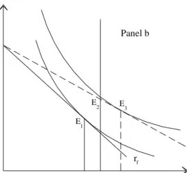
Figure 2: Rental demand under control c hc Panel a h y rc rf E3 E 2 1 E 1 h h3 h1hc h3 y c 1 E 2 E 3 f r E Panel b h rc
This result is illustrated in figure 2 panel a, where the dashed line from y illustrates the budget restriction under controlled rent, and the solid more negatively sloped line illustrates the budget restriction under free market rent. The two goods in the utility function are housing h and other consumption c. With other consumption having the price 1, y is the real value of household income measured in units of other consumption. Housing demand is assumed to be a normal good with an increasing demand when the rent is falling. Therefore, the demand increases from h1 to h3 when the rent falls from rf to rc. However, if the household is offered only the amount hc of controlled housing to the rent rc this offer is accepted because the welfare is higher in E2 than in E1. If this kind of rationing dominates the observations in our
sample, we will see a drop in the demand among households in apartments with controlled rent compared to households (with same characteristics) in the uncontrolled market sector who on average will consume h1. However, if controlled housing is offered amply, the picture
of panel b occurs, and households in apartments with rent control occupy more housing than they would on the market sector without rent control. Panel b of figure 2 shows a case where rent controlled housing is offered amply compared to housing without rent control.
Table 6: Paid rent compared to market rent per square meter Type of rental housing Paid rent rc Calculated market rent1)
rf
Difference as per cent of market rent
- supported housing 484.2 567.9 -14.7
- controlled rent 475.9 545.4 -12.7
- damped rent 476.6 491.8 -3.3
Notes: See also figure 2. Rents are the average annual rent in DKK per square meter for each sector in year 1999. 1) Calculated rent for the cleaned sample by use of the coefficients in table 3. The difference in the paid rent between the sectors depends both on the design of the control system and on the specific characteristics of the dwellings.
To look into this, we first calculate the average predicted (market) rent per square meter, following the estimated equation of table 3, for the rent controlled sectors, and compare this with the average rent per square meter actually paid in the sectors. Table 6 shows the result. As expected, actual rents paid in the controlled sectors are lower than the free market rent for similar dwellings. The difference is largest for supported housing with a paid rent per square meter, which is 14.7 per cent under the rent, had the square meters been offered on the free market. Also for controlled private letting is there a clear difference, whereas rental housing with damped rent seems to have a rent more in line with the market rent. Skifter Andersen (2008) interviewed 385 private landlords with properties containing 3 and more dwellings, who on average predicted a 10 per cent increase in rents if control was abolished. Our estimates are broadly in line with this. In relation to figure 2, the table confirms that rents in controlled sectors of the market are below the free market rent as shown by the slope of the budget lines in the figure.
Figure 3 shows the kernel density functions for the estimated rents in the controlled sector and the density function for the actual rents in the market sector. The figure demonstrates that the estimated rents are within the range of the free market rents.
Figure 3: Density of estimated rents for controlled sectors and actual rents for the market sector
Notes: The figure shows the density of estimated rents by use of the coefficients in table 3 for the three market sectors with supported housing, with controlled rent and with damped rent, and the density of actual rents for dwellings in the market sector.
In order to show the number of allocated square meters hc compared to the quantity demanded
h3 under controlled rent, h3 is calculated in table 7 by use of the estimated relation in table 4. Thus, it is assumed in table 7 that the regression based on market sector observations reveals the demand for square meters area for households in other sectors. The table shows that neither in supported housing nor in private controlled rental housing are households on average allocated a number of square meters that surpasses the quantity demanded under controlled rent. In the sector with damped rent, allocations are more in line with the quantity demanded, but with an average overallocation of 2.3 per cent. With reference to the figure 2, the number of allocated square meters hc is on average lower than the demanded number of square meters h3 in supported and private controlled housing, but slightly higher than the quantity demanded in the sector with damped rent.
Table 7: Actual allocation and demanded amount of square meters Type of rental housing allocation hActual
c
Calculated quantity demanded at paid rent1) h3
Overallocation, per cent2)
- supported housing 76.23 79.57 -4.2
- controlled rent 72.92 77.28 -5.6
- damped rent 79.70 77.90 2.3
Notes: See also figure 2. The table shows the average number of square meters area. 1) Calculated quantity demanded for the cleaned sample by use of coefficients from table 4. 2) Per cent of calculated quantity demanded.
A final exercise is to compare hc and h1 in figure 2, i.e. the allocated number of square meters compared to the quantity demanded had the square meters been offered in the sector with market rent. The market rent is estimated by use of the coefficients in table 3 and with this, the quantity demanded h1is calculated by the use of the coefficients in table 4. The increase of the rent from controlled to market rent should by itself reduce the quantity demanded. But, as table 8 reveals, restrictions on the offered number of square meters in supported housing12 has the consequence that allocations do not differ much from the quantity demanded, had the square meters been offered on the sector with market rent. This corresponds to panel b of figure 2, where hc lies to the right of h1, but to the left of h3. The private rent controlled sector is also pictures in panel b. The explanation behind the lack of overallocation in this sector must be that the low rent makes the housing units so attractive that households accept fewer square meters than the quantity demanded, but still get a welfare gain compared to renting in the uncontrolled sector of the market. Finally, the sector with damped rent has hc to the right of h3 and so even further away from h1. Here the average overallocation is 6.4 per cent. One should also expect to find incidences of overallocation in the market sector when calculated as in table 6. Part of this is caused by discontinuities of the supplied number of square meters with the consequence that a number of households in demand for housing will have to accept more or fewer square meters than demanded at the offered rent. However, it seems reasonable to assume that a market with no control is better to meet idiosyncratic differences between the households than a system with control and administrative or random
12
In supported housing, a single person is offered an apartment with two rooms. Three rooms may be offered to married or cohabitating couples if so decided by the local supported housing department. Apart from this, three and more rooms are reserved for households with children. Furthermore, low income households can apply for public support for an entrance deposit. Most supported housing departments have waiting lists for new tenants, but allow internal rotation between incumbents before admission of new tenants.
allocation. Hence, a big part of a calculated overallocation in the market rent sector is not welfare reducing overallocation, but a reflection of idiosyncratic household differences. In the rent controlled sectors we postulate a welfare reducing misallocation if the allocated square meters exceed the individual household’s quantity demanded under an uncontrolled rent for the dwelling.
Table 8: Actual allocation and demanded amount of square meters at market rent Type of rental housing allocation hActual
c
Calculated quantity demanded at market rent1) h1
Overallocation, per cent2)
- supported housing 76.23 75.69 0.8
- controlled rent 72.92 72.47 0.6
- damped rent 79.70 74.58 6.4
Notes: See also figure 2. The table shows the average number of square meter area. 1) Calculated quantity demanded for the cleaned sample by use of coefficients from table 4 and uncontrolled market rents estimated by use of coefficients from table 3. 2) Per cent of calculated quantity demanded at market rent.
To give an impression of the degree of welfare reducing overallocation, we calculate the number of over- and underallocated square meters for all households in table 9 using the same technique as in table 8. We have also included a column for the market sector in the table to illustrate the calculations for this sector. But based on the reasoning above, we do not consider the overallocation in this sector as welfare reducing overallocation. Among the rent controlled sectors, the amount of overallocation ranges between 9.4 and 16.4 per cent of actual
allocations, with the highest degree of overallocation found in the sector with damped rent.
Table 9: Calculated over- and underallocation of square meters area Supported housing Controlled rent Damped rent Market rent Actual allocations 6 149 816 1 811 565 631 725 332 645 Sum of underallocations 525 102 204 470 63 868 28 346 Sum of overallocations 577 498 211 534 103 700 40 959 Net overallocations 52 396 7064 39 832 12 613
Overallocations, per cent1) 9.4 11.7 16.4 12.3
Potentially, all overallocations under rent control are welfare reducing, but we cannot exclude that part of the overallocation is given to households with an idiosyncratic high preference for housing, which is not captured by the control variables in our estimations. But it is also so that the result in table 9 covers a number of individual and in the public eye scandalous
overallocations in the controlled market sectors. In order to give an impression of this, we have calculated the mean overallocation among households who have overallocation of square meters, see table 10.
Table 10: Mean under and overallocation of square meters area per under and overallocated household respectively, percentages in brackets.
Supported housing Controlled rent Damped rent Market rent Actual allocations 76.23 72.92 79.70 73.87
Under allocated households 13.31 14.63 16.06 12.82
Over allocated households1) 14.64(19) 19.09(26) 25.95(33) 17.87
20 per cent most over allocated1) 31.94(42) 53.18(73) 73.01(92) 47.84
Welfare loss from overallocation2) 612.7(1.7) 663.4(1.9) 197.2(0.5) Welfare loss from overallocation among
the 20 per cent most overallocated2) 1336.7(3.6) 1848.0(5.3) 554.9(1.5)
Note: Mean allocations per household in all dwellings, in under and overallocated dwellings, and the mean among the 20 per cent most overallocated households. 1) Per cent of actual allocations for the average household in the bracket. 2) Kroner per year and per cent of annual rent for the average household in the bracket.
The table repeats the picture of table 9. Most overallocation is found in the sector with
damped rent. Among the 20 per cent most overallocated households, it amounts to 42 per cent for supported housing, increasing to 92 per cent or close to a doubling of the average size in the sector with damped rent.
Table 10 also contains a crude calculation of the welfare loss per households from overallocation. Taking the sector with damped rent, the calculation is the following:
households are assumed to value the last allocated square meter to 476.6 kroner13, see table 6. The households are on average overallocated 25.95 square meters. Therefore, with 25.95 square meters less they value the marginal square meter to the free market rent, i.e. 491.8 kroner. The market value for each of the 25.95 square meters is 491.8 kroner. With a linear
13
This is an approximation; table 7 reveals that the valuation is on average lower for overallocated households in the sector with damped rent. It is higher in supported housing and the sector with controlled rent.
demand curve, the welfare loss can be calculated as the area of a triangle above the demand curve equal to ½(491.8-476.6)25.95 = 197.2 kroner or ½ per cent of the annual rent for the dwelling of an average household in the sector14. The welfare loss is influenced by the difference between the controlled rent and the market rent and this has the implication that now the private rent controlled sector comes in front with the highest welfare loss. For the 20 per cent most overallocated households in this sector, the welfare loss is 5.3 per cent of the average annual rent.
6. Conclusion
Misallocation is expected in rent controlled housing because households who value housing most may not be allocated the dwellings. No rental housing sector, controlled or uncontrolled can offer every household exactly the demanded number of square meters. Discontinuities of supply, asymmetries of information and transaction costs have the consequence that
incidences of over- and underallocation of square meters can be found in all sectors of the market. However, with rent control applied in a sector of a homogenous rental housing market only overallocation among households in controlled dwellings should be counted as welfare reducing misallocation.
Our method differs from the estimations done by Glaeser and Luttmer (2003) for the New York City. They compare rental markets between metropolitan areas with and without rent control and estimate that approximately 20 per cent of all apartments in the New York City are overallocated in terms of number of rooms. We take the actual segregation of the Danish rental housing market as the basis for the analyses and calculate welfare reducing
overallocation among households in controlled housing units as the surplus of actual
allocation of square meters minus the quantity demanded, had the square meters been offered on the free market rent sector. We find no tendency for net overallocation in supported housing and in the private rent controlled sector of the market, and explain this partly with a restrictive administrative allocation system in supported housing, and partly because the low rent in controlled sectors may make the dwellings so attractive that households accept fewer square meters than the quantity demanded, and still get a welfare gain compared to renting on the free market. However we find welfare reducing overallocation in the controlled sectors between 9 and 17 per cent of actual allocations. Looking at the 20 per cent most overallocated
14
Adding up to the country level, the welfare loss from overallocation is approximately 12 mill kroner per year in this sector.
households; we find overallocations of square meters ranging between 42 and 92 per cent of the average allocation per household, and estimate the corresponding welfare losses to be from 1.5 to 5.3 per cent of the average annual rent in the sectors.
References
Arnott, Richard (1995): Time for Revisionism on Rent Control. Journal of Economic Perspectives. Vol. 9, No. 1, Winter 1995, pp. 99-120.
Fallis, George and Lawrence B. Smith (1984): Uncontrolled Prices in a Controlled Market: The Case of Rent Controls. The American Economic Review. Vol. 74, No. 1, March 1984, p. 193-200.
Glaeser, Edward L. (1996): The Social Costs of Rent Control Revisited. National Bureau of Economic Research (Cambridge, MA) Working Paper No. 5441, January 1996.
Glaeser, Edward L. and Erzo F.P. Luttmer (1997): The Misallocation of Housing under Rent Control. National Bureau of Economic Research (Cambridge, MA) Working Paper No. 6220, October 1997.
Glaeser, Edward L. and Erzo F.P. Luttmer (2003): The Misallocation of Housing under Rent Control. The American Economic Review. Vol. 93, No. 4, September 2003, p. 1027–46.
Gyourko, Joseph and Peter Linneman (1990): Rent controls and rental housing quality: A note on the effects of New York City's old controls. Journal of Urban Economics. Vol. 27, Issue 3, May 1990, p. 398-409.
Hubert, Franz (1993): The Impact of Rent Control on the Rents in the Free Sector. Urban Studies. Vol. 30, No. 1, p. 51-61.
Häckner, Jonas and Sten Nyberg (2000): Rent Control and Prices of Owner Occupied Housing. Scandinavian Journal of Economics. Vol. 102, No. 2, p. 311-24.
Ng, Yew-Kwang (1979): Welfare Economics. The Macmillan Press Ltd. London.
Marks, Denton (1984): The Effect of Partial-coverage Rent Control on the Price and Quantity of Rental Housing. Journal of Urban Economics. Vol. 16, Issue 3, November 1984, p. 360-69.
Sims, David P. (2007): Out of control: What can we learn from the end of Massachusetts’s rent control? Journal of Urban Economics. Vol. 61, Issue 1, January 2007, p. 129-59.
Madsen, Bent (2006): Skal den almene boligsektor gøres fri. Samfundsøkonomen. No. 4, Oktober, pp. 31-34.
Skak, Morten (2008): Projecting Demand for Rental Homes in Denmark. European Journal of Housing Policy. Vol. 8, Issue 3, Sep2008, p. 235-62.
Skifter Andersen, Hans (2007): Private udlejningsboligers rolle på boligmarkedet: En registeranalyse (SBi 2007:13). Hørsholm: Statens Byggeforskningsinstitut, Aalborg Universitet.
Skifter Andersen, Hans (2008): Is the Private Rented Sector an Efficient Producer of Housing Service? Private Landlords in Denmark and their Economic Strategies. European Journal of Housing Policy, Vol. 8, Issue 3, Sep2008, p. 263-86.
Appendix
Table A1: Variable description
Name Type Description
Area per household continuous square meters of dwelling area
Ln of area continuous natural logarithm of area per household
Rent per sqm. continuous rent in DKK per square meter per year Ln rent per sqm. continuous natural logarithm of rent per sqm Age of building continuous age of building in years
Age of building squared continuous squared age
Attached dummy dwelling is in an attached building
Detached dummy dwelling is in a detached building
Semi detached dummy dwelling is in a semi detached building
Length of tenure continuous length of tenure in years for the person with highest length Square of length of tenure continuous square of length of tenure
Income per equivalent person continuous total household disposable income divided by number of equivalent persons
Ln income per equivalent person continuous natural logarithm of income per equivalent person Number of equivalent persons continuous (number of adults + 0.6 times the number of children)^0.8 Square of number of equivalent
persons
continuous square of number of equivalent persons Age or breadwinner continuous age of breadwinner
Age or breadwinner squared continuous square of age of breadwinner
No education dummy breadwinner has no education
Short education dummy breadwinner has short education
Long education dummy breadwinner has long education
Wage earner dummy breadwinner is wage-earner
Self employed dummy breadwinner is self-employed
Undergoing education dummy breadwinner is under education
Pre pensioner dummy breadwinner is under pre pension
Social pensioner dummy breadwinner receives social pension
Early pensioner dummy breadwinner is early pensioner
Old age pensioner dummy breadwinner is old age pensioner
Immigrant dummy breadwinner is immigrant
Single dummy breadwinner is single
Married dummy breadwinner is married
Divorced dummy breadwinner is divorced
Widow dummy breadwinner is widow/-er
Completely urbanized dummy urbanization degree1 95 – 100%
Highly urbanized dummy urbanization degree 80 – 95%
Medium urbanized dummy urbanization degree 55 – 80%
Low urbanized dummy urbanization degree 0 – 55%
Built-up roof dummy building has built-up roofing and/or roofing felt Vacancy rate continuous share of vacant dwellings in municipality, %
Table A2: Descriptive statistics for the 20 per cent random sample minus the sector with coop ownership
Name Obs Mean Std. Dev. Min Max
Rent per sqm. 126,114 487.57 337.92 23.15 47661.5
Ln of rent per sqm. 126,114 6.14 0.29 3.14 10.77
Area per household 163,673 80.38 38.57 18 3450
Ln of area 163,673 4.31 0.39 2.89 8.15 Age of building 160,930 48.0 36.30 1 499 Attached 164,291 0.72 0.45 0 1 Detached 164,291 0.09 0.29 0 1 Semidetached 164,291 0.19 0.39 0 1 Length of tenure 164,291 12.5 17.13 1 102
Income per equivalent person 163,719 167,064.8 176,235.2 1 9,853,900
Ln of income 164,291 11.82 0.60 0 16.10 Equivalent persons 164,291 1.48 0.63 1 18.4 Age of breadwinner 164,291 48.27 19.38 0 113 No education 164,291 0.54 0.50 0 1 Short education 164,291 0.36 0.48 0 1 Long education 164,291 0.10 0.30 0 1 Wage earner 164,291 0.49 0.50 0 1 Self employed 164,291 0.02 0.15 0 1 Undergoing education 164,291 0.03 0.16 0 1 Pre pensioner 164,291 0.10 0.30 0 1 Social pensioner 164,291 0.06 0.23 0 1 Early retirement 164,291 0.03 0.17 0 1
Old age pensioner 164,291 0.21 0.41 0 1
Immigrant 164,291 0.10 0.30 0 1 Single 164,291 0.41 0.50 0 1 Married 164,291 0.28 0.45 0 1 Divorced 164,291 0.18 0.39 0 1 Widow 164,291 0.13 0.34 0 1 Completely urbanized 164,291 0.55 0.50 0 1 Highly urbanized 164,291 0.24 0.43 0 1 Medium urbanized 164,291 0.18 0.39 0 1 Low urbanized 164,291 0.03 0.16 0 1 Built-up roof 162,321 0.19 0.39 0 1 Vacancy rate 164,291 6.14 2.49 1.2 23.8