The Effects Of Monetary Policy Shocks In Peru: Semi-Structural Identification Using A Factor-Augmented Vector Autoregressive Model

BANCO CENTRAL DE RESERVA DEL PERÚ

The Effects Of Monetary Policy Shocks In Peru:

Semi-Structural Identification Using A

Factor-Augmented Vector Autoregressive Model

Erick Lahura*

* Central Bank of Peru and LSE

DT. N° 2010-008

Serie de Documentos de Trabajo

Working Paper series

Julio 2010

Los puntos de vista expresados en este documento de trabajo corresponden al autor y no reflejan necesariamente la posición del Banco Central de Reserva del Perú.

The views expressed in this paper are those of the author and do not reflect necessarily the position of the Central Reserve Bank of Peru.

THE EFFECTS OF MONETARY POLICY SHOCKS IN PERU:

SEMI-STRUCTURAL IDENTIFICATION USING A FACTOR-AUGMENTED VECTOR AUTOREGRESSIVE MODEL

Erick W. Lahura1

(Central Bank of Peru and LSE) May, 2010

Abstract

The main goal of this paper is to analyze the effects of monetary policy shocks in Peru, taking into account two important issues that have been addressed separately in the VAR literature. The first one is the difficulty to identify the most appropriate indicator of monetary policy stance, which is usually assumed rather than determined from an estimated model. The second one is the fact that monetary policy decisions are based on the analysis of a wide range of economic and financial data, which is at odds with the small number of variables specified in most VAR models. To overcome the first issue, Bernanke and Mihov (1998) proposed a semi-structural VAR model from which the indicator of monetary policy stance can be derived rather than assumed. Meanwhile, the data problem has been resolved recently by Bernanke, Boivin and Eliasz (2005) using a Factor-Augmented Vector Autoregressive (FAVAR) model. In order to capture these two issues simultaneously, we propose an extension of the

FAVAR model that incorporates a semi-structural identification approach a la Bernanke

and Mihov, resulting in a VAR model that we denominate SS-FAVAR. Using data for Peru, the results show that the SS-FAVAR's impulse-response functions (IRFs) provide a more coherent picture of the effects of monetary policy shocks compared to the IRFs of alternative VAR models. Furthermore, it is found that innovations to nonborrowed reserves can be identified as monetary policy shocks for the period 1995-2003.

Keywords: VAR, FAVAR, Monetary Policy, Semi-Structural Identification. JEL classification: C32, C43, E50, E52, E58

1 _{The author will like to thank Paul Castillo, Alberto Humala and Marco Vega for their comments and}

suggestions. The views in this paper are those of the author and do not necessarily represent those of the Central Bank of Peru or LSE. Comments are very welcome. E-mail: [email protected].

1. Introduction

In economics, the Vector Autoregressive (VAR) framework is the standard tool

to analyze the effects of monetary policy shocks2. This approach was first proposed by

Sims (1980) and applied to monetary policy analysis by authors like Bernanke and Blinder (1992), Sims (1992), Christiano and Eichenbaum (1992), Gordon and Leeper (1994), Strongin (1995), Lastrapes and Selgin (1995) and Gerlach and Smets (1995), Leeper, Sims and Zha (1996), Bernanke and Mihov (1998), Sims and Zha (1998), Christiano, Eichenbaum and Evans (1999), among others.

Two main issues have surrounded the analysis of the effects of monetary policy shocks using VAR models: (i) the difficulty in identifying the most appropriate indicator of monetary policy stance and thus identifying monetary policy shocks, and (ii) the correct specification of the empirical model, which is restricted by the limited number of variables that can be included in a standard VAR.

In general, the indicator of monetary policy stance is assumed rather than determined from an estimated model, and is usually identified through changes in an interest rate or monetary aggregate under the control of the central bank. However, Bernanke and Mihov (1998) proposed a VAR-based methodology in which the indicator of monetary policy stance is obtained from an estimated model of the central bank‟s operating procedure. In particular, they employed a „semi-structural‟ VAR model where there are some contemporaneous identification restrictions on a set of variables that describe the market for commercial bank reserves, leaving the relationship among the rest of macroeconomic variables unrestricted. We refer to this as the "semi-structural" identification approach. The main result of this approach is that the indicator of monetary policy stance may not be uniquely determined by one variable (e.g. interest rate or some monetary aggregate) but may be related to a group of variables, depending on the central bank's operating procedures.

2 _{As stated by Bernanke and Mihov (1998) and Christiano et al. (1999), the VAR approach focuses on}

policy shocks and not the systematic component of monetary policy or “policy rule”. The main reason is that tracing the dynamic response of the economy to a monetary policy innovation allows to observe the effects of policy changes under minimal identifying assumptions. An alternative approach to analyze monetary policy is the so-called “narrative approach” (Friedman and Schwartz, 1963; Romer and Romer, 1989). See Christiano et al. (1999) for a good survey.

On the other hand, the fact that monetary policy decisions are based on the analysis of a wide range of economic and financial data is at odds with the specification of a small number of variables in most VAR models. In principle, the more variables that are specified in the VAR, the less degrees of freedom will remain and the less precise (higher standard errors) the estimates will be. This is the main reason why most VAR models are restricted to a reduced number of variables (up to 6 in most cases).

Bernanke et al. (2005) point out two main problems that could arise using the standard VAR approach that considers only a small number of variables. First, it is possible that policy shocks are measured with error, mainly because the limited number of variables specified in a VAR may not reflect the full spectrum of information used by central banks and private agents. In this case, it would not be rare to observe some of the so-called “puzzles” that arise in standard VAR analysis. Second, the impulse-response analysis is restricted to the variables specified in the VAR model, which in turn raises two problems. On the one hand, it may be the case that the specified

variables do not correspond to the theoretical ones3. On the other hand, it is often

relevant to analyze the response of a wide range of variables that summarize the state of the economy.

One way to deal with these problems is combining the standard VAR analysis with “factor analysis”, as recently proposed by Bernanke et al. (2005), which results in the so-called Factor Augmented Vector Autoregression (FAVAR) model. Stock and Watson (2002) and Bernanke and Boivin (2003), show that factor analysis allows us to summarize a large amount of information in a small number of factors. Thus, including these “few” factors in standard VAR methodology makes feasible the inclusion of the whole range of economic information used by central banks into VAR analysis.

In the case of Peru, the analysis of the effects of monetary policy using VAR analysis has faced the same two problems. On one hand, the difficulty to identify the indicator of monetary policy stance has been mainly related to: (a) the use of different operational procedures and instruments following the period of hyperinflation (1987-1990), featuring the announcement of an interest rate corridor in 2001 and the use of an

3

For instance, detrended real output (obtained using HP filtering in many cases) may not correspond to the theoretical “output gap”.

official interest rate as the policy instrument in September 2003, and (b) the change

from a monetary targeting regime -implemented in 19914- to an explicit inflation

targeting regime in January 2002. On the other hand, the partially dollarized nature of the economy means that an even greater number of variables need to be specified compared to the existing VAR models, an issue that falls into the second problem discussed above.

Previous research on monetary policy in Peru based on VAR models assume a

priori an indicator of monetary policy and restrict the number of variables employed in the analysis. León (1999), using different VAR models with 5 or less variables and a Cholesky identification strategy, provides evidence that monetary aggregates affect inflation; in particular, he finds that a change in the growth rate of M1 raises inflation with a time lag of between 4 and 14 months. Quispe (2000) and Castillo and Pérez (2010) apply the Bernanke and Mihov approach taking into account the dollarized nature of the Peruvian economy. In particular, Quispe (2000) finds that the high degree of asset dollarization does not affect the power of monetary policy using monetary aggregates, showing that money affects inflation between 8 to 16 months after the shock. Rossini (2001), using a standard VAR with five variables, finds that fifty percent of a shock to monetary base is transmitted to inflation after 5 quarters. Finally, Winkelried (2004), using a cointegrated-VAR approach with 7 variables and assuming that the interest rate can measure the monetary policy stance from 1993 to 2003, finds that a shock to interest rate affects output and inflation after one year, considering data from 1993 to 2003.

Our aim is to contribute to the analysis of monetary policy in Peru taking into account the two main issues mentioned above simultaneously. In order to do it, we propose an extension of the FAVAR model that incorporates a semi-structural

identification approach a la Bernanke and Mihov, resulting in a VAR model that we

denominate SS-FAVAR. Using data for Peru, the results show that the SS-FAVAR's impulse-response functions (IRFs) provide a more coherent picture of the effects of monetary policy shocks compared to the IRFs of alternative VAR models.

The paper is structured as follows. In section 2 we present and discuss the semi-structural identification framework proposed by Bernanke and Mihov (1998). The FAVAR model proposed by Bernanke, et al. (2005) is presented in section 3. In section 4, the FAVAR model is extended using Bernanke and Mihov's identification strategy, obtaining what we denominate a SS-FAVAR model. In section 5 we present and analyze the main results obtained from these three approaches. Finally, we summarize our main conclusions in section 6.

2. Structural (non recursive) VAR identification and the market for bank reserves

There are many investigations that have studied the impact of monetary policy shocks based on assumptions about the central bank‟s operating procedures in the market for bank reserves. Some important papers for the U.S. economy are Bernanke and Blinder (1992), Christiano and Eichenbaum (1992), Cosimano and Sheehan (1994) and Strongin (1995), and Bernanke and Mihov (1998) who proposed a unified framework that nests all these previous studies, based on a small semi-structural model for bank reserves. Despite some potential weakness of this approach (see Christiano et al. 1999), it is still quite useful to understand the effects of monetary policy shocks on the economy.

2.1. Basic Framework: Unrestricted VAR

It is assumed that the structure of the economy can be described by the following unrestricted dynamic model:

(1) y _ty q i i t i q i i t i t BY CP A v Y 









where Y_t is a vector of macroeconomic variables (non policy variables), and P _t is a

vector of possible monetary policy indicators, both vectors dated at time t. The vectors

y t

v and vtp contain structural (or primitive) disturbances which are assumed to be

mutually uncorrelated; the presence of the matrixes Ay and AP imply that shocks may

enter into more than one equation.

Equation (2) states that the set of policy indicators Pt depend on current and

lagged values of Y_t and P_t, and on a set of disturbances p

t

v . Bernanke and Mihov (1998)

assume that one element of the vector vtp is a money supply shock or policy disturbance

s t

v , while the remaining elements of p

t

v may include shocks to money demand or other

nonpolicy variables Y_t to depend on current and lagged values of Y_t and P_t. Thus the system (1)-(2) is not identified.

One possible identification procedure is to allow the nonpolicy variables to

depend only on lagged values of policy variables, which implies that C0 0

5

. Under this assumption, the system is given by:

(1a) _{t i} y _ty q i i q i i t i t BY CP A v Y   _    









To analyze the dynamic responses of variables to a policy shock s

v , we can

rewrite the system (1a)-(2) as a standard VAR, with only lagged variables on the right-hand side: (3) _t 1 t t t t u P Y Φ(L) P Y               

where Φ

 

2.2. Identification of policy shocks: the market for bank reserves

Let u_tp be the portion of the VAR residuals in the policy block that is orthogonal

to the VAR residuals in the non-policy block, which satisfies:

(4) u_tp 





or, dropping subscripts and superscripts:

(5) uGuAv

5

This is analogous to the identifying assumption made in Bernanke and Blinder (1992), where Pt is a

Equation (5) is a standard structural VAR (SVAR) system, which relates

observable VAR-based residuals u_t to unobserved structural shocks v_t, one of which is

the policy shock s

t

v . Thus, given C₀ 0, the identification of the monetary policy

shock _vs _{implies the identification of matrixes G and A.}

For this purpose, and following Bernanke and Mihov (1998) and Christiano et al. (1999), we consider the following model (in innovation form) that describes the market for bank reserves:

(6) d IIR TR u v u   (7) uNBR dvd bvb vs (8) u_BR (u_IIR u_DISC)u_NBR vb

where u denotes an (observable) VAR residual and v indicates an (unobservable)

structural disturbance.

The banks‟ total demand for reserves6 is represented by equation (6). In this

equation, the innovation in the demand for total reserves u_TR depends (negatively) on

the innovation in the interbank interest rate7 (the price of reserves) and on a demand

disturbance vd.

The behaviour of the central bank is described by equation (7). It is assumed that the central bank observes and responds to shocks to the total demand for reserves and to

the demand for borrowed reserves, and to exogenous “monetary policy” shocks s

v .

Finally, equation (8) represents the banks‟ demand for borrowed reserves8. The

innovation in the demand for borrowed reserves u_BR depends positively on the

6 _{Total reserves is the amount of money held at the central bank by the private banks. Borrowed reserves}

is the amount of money borrowed by banks through the central bank's discount window, in order to meet the required level. Nonborrowed reserves is the difference between total reserves minus borrowed reserves.

7 _{The interbank interest rate is analogous to the federal fund rate in FED system.} 8

Borrowed reserves is defined as the portion of reserves that banks choose to borrow at the discount window.

innovation in the interbank interest rate u_IIR (the rate at which borrowed reserves can be

relent), negatively on both the discount rate innovation u_DISC (the cost of borrowed

reserves), and nonborrowed reserves innovation uNBR

9

, and on a borrowing disturbance

b

v . Given that nonborrowed reserves are the difference between total reserves and

borrowed reserves, the innovation in nonborrowed reserves u_NBR is u_TRu_BR, so

equation (8) can be written as:

(8a) u_TRu_NBR (u_IIR u_DISC)u_NBRvb

Using the conventional assumption that innovations to the discount rate are

zero10, we can re-write (6), (7) and (8a) in terms of u_TR, u_NBR , u_IIR in the following

structural form:                                                              b s d b d IIR NBR TR IIR NBR TR v v v u u u u u u 1 0 0 1 0 0 1 ) 1 ( ) 1 ( 1 0 0 0 0 0 or: (9) uGuAv

The solution of this system in terms of innovations11 is:

                                                                                                                        b s d b d b d b d IIR NBR TR v v v u u u 1 ) 1 ( 1 1 ) 1 ( 1 ] 1 ) 1 ( [ ) 1 ( ) 1 (

9 _{Christiano et al. (1999) consider this term based on the results of standard dynamic models of the market}

for reserves (e.g. Goodfriend (1983), which provide evidence that 0. However, Bernanke and Mihov assume that 0.

10 _{See Bernanke and Mihov (1998), p. 877, footnote 10, for a discusión of this simplifying assumption.} 11

It is assumed that the supply of nonborowed reserves plus borrowings must equal the total demand for reserves, as in Bernanke and Mihov (1998).

or:

(10) u{[I G]1A}v

If we know the values of the parameters ,,d,b and  (and hence the matrix

A G

I ] 1

[   ), using the estimated reduced-form residuals u'[u_TR u_NBR u_IIR], we can

obtain an estimation of the structural shocks v'[vd vs vb] calculating

u A G I v{[  ]1 }1 : (11)





In particular, the monetary policy shock vs, which is given by:

(12) vs (d b)u_TR(1b[1])u_NBR (d b)u_IIR

The model represented by (12) has eight unknown parameters: ,,d,d,

and the variances of the three structural shocks. These parameters can be calculated

from the estimated variance covariance matrix of the reduced-form residuals vector u,

which is diagonal and has six different covariances; thus, the model is “underidentified”: we have only six pieces of information to find eight unknowns. Then, in order to identify the model we need at least two more restrictions (if this is the case then model is exactly identified). However, Bernanke and Mihov (1998) assume

implicitly that 0, so the structural model becomes:

                                                           b s d b d IIR NBR TR IIR NBR TR v v v u u u u u u 1 0 0 1 0 0 1 ) 1 ( 1 1 0 0 0 0 0 or:

(9a) uGuAv which implies:                                                                                                                                       b s d b d b d b d IIR NBR TR v v v u u u ) 1 ( 1 1 ) 1 ( 1 1 ) 1 ( 1 ) 1 (

and in terms of the structural disturbances:

(11a)





In this case, the monetary policy shock vs is given by:

(12a) IIR b d NBR b TR b d s u u u v (  ) (1 ) (  )

Now, the structural model has only seven unknown parameters: ,,d,d and

the variances of the three structural shocks, so we need only one restriction to exactly identify the model. In this context, Bernanke and Mihov (1998) consider five alternative (non-recursive) identification schemes which correspond to four indicators of policy proposed in the literature (each of which provides overidentification) and one just-identified alternative which allows a general policy indicator. We consider the following ones:

 Model 1: FFR (federal funds rate). Analogous to the one used in Bernanke and

Blinder (1992). According to this model, if the central bank targets the interbank interest rate (federal fund rate in the case of U.S.), then the central bank offsets shocks to total reserves demands and borrowing demands. This case corresponds

monetary policy shock is proportional to the innovation to the interbank interest

rate: IIR

s

u v () .

 Model 2: NBR (nonborrowed reserves). In this model, it is assumed that

innovations to nonborrowed reserves mainly reflect exogenous shocks to monetary policy, while innovations to broader monetary aggregates reflect shocks to money demand (Christiano and Eichenbaum, 1992). These

assumptions correspond to the overidentifying restrictions d b 0. In this

case, the monetary policy shock is just the reduce-form innovation in the

nonborrowed reserves s _NBR

u

v  .

 Model 3: NBR/TR (“orthogonalized’’ nonborrowed reserves12). Following

Strongin (1995), it is assumed that shocks to total reserves are purely demand

shocks13, 0, and that the central bank doesn‟t respond to borrowing shocks,

0

 b

. Thus, these two overidentifying assumptions imply that the monetary

policy shocks are given by vs du_TRu_NBR.

 Model 4: BR (borrowed reserves). Borrowed-reserves targeting corresponds to

the restrictions φd 1,φbα/β. Alternatively, we can use φd1,φb 0,0

(so that 0 is possible). In the latter, the implied monetary policy shock is

proportional to the negative of the innovation to borrowed reserves

BR NBR TR s u u u v (  ) .

 Model 5: JI (Just-identification). In order to get a just-identified model,

Bernanke and Mihov (1998) consider only 0. In this case, the implied

monetary policy shock is a linear combination of the innovations to the three

policy variables considered: b _IIR

NBR b TR b d s u u u v (  ) (1 )  12

The name "orthogonalized" comes from the idea that shocks can be identified having total reserves immediately precede nonborrowed reserves in a standard Cholesky decomposition. Thus, the policy shock can be identified as the "orthogonalized" error in the nonborrowed reserves equation.

13

In the short run, the central bank has no choice but to “accommodate” to total reserves shocks, using either open-market operations or the discount window.

Each model presented above is overidentified by one restriction (except Model 4) with respect to equation (12a). Therefore the validity of any model, can be assessed

using a test of the overidentifying restrictions. Thus, the rejection of the test14 implies

the rejection of the model considered.

2.3. Some general criticisms

Christiano, L; Martin Eichenbaum and Charles Evans (1999), or CEE (1999), point out a potential weakness in the identification procedure proposed by Bernanke and Mihov (1998), based on the test of overidentifying restrictions. CEE state that the rejection of the test can always be interpreted as evidence against the maintained

hypothesis 0 with respect to system (9) rather than evidence against one of the

identification schemes. Thus, CEE conclude that a rejection of an overidentifying test in this context is not evidence against a given identification schemes mentioned above;

this is true only if we have the prior that 0.

Furthermore, even if it is assumed that 0, CEE points out that there is a

problem to test the validity of the restrictions implied by Models 1, 2 and 3, using

standard statistical procedures. The reason is that the system (9), where 0, is exactly

identified under Model 1, 2 or 3, so an overidentifying restrictions test is not valid. In this case, CEE recommend the comparison of the corresponding impulse-response functions as a strategy to assess the validity of the competing models.

However, CEE‟s proposed solution requires implicitly a correct specification of the VAR model, and thus the problem of how many variables should be included in the VAR arises (although this problem is not restricted to CEE‟s criticism only). As mentioned in section1, a way to deal with these data problem is using the Factor-Augmented Vector Autoregression (FAVAR) model, which makes feasible the inclusion of a wide range of economic information into a standard VAR model, through the inclusion of a small number of factors. In the next section we present the key aspects of the FAVAR approach.

14

The null hypothesis is that the specified restrictions implied by a particular model are valid (i.e., the specified model is valid).

3. Factor-Augmented Vector Autoregressive (FAVAR) approach

The main feature of the FAVAR approach is that it allows the inclusion of a huge number of variables in the VAR framework, through the use of “factor analysis”. In the next subsection we present briefly the general framework, the estimation and

identification of a FAVAR model15.

3.1. General framework

Let us assume that there are a “small” number M of observable economic

variables that determine the dynamics of the economy, contained in the vector Y_t

(𝑀𝑥1). Then the dynamics of the economy can be analyzed using a Vector Autoregressive (VAR) model of the form:

(13) ) 1 ( ) 1 ( 1 ) ( ) 1 ( ) ( Mx t Mx t MxM Mx t L Y v Y  _ 

where (L) is a conformable lag polynomial of order d. However, in many

applications, additional economic information not included in Y_t may be relevant to

modelling the dynamics of these series. Let us suppose that this additional information

obtained from observed economic variables (time series) is included in a N1 vector

t

X , where N is a large number Furthermore, assume that this “large” number of

“observed” informational variables can be compressed into a “small” number K of

unobserved factors and the “small” number M of economic variables contained in Yt,

as follows:

(14) X_t fF_t yY_t e_t , t 1,,T

where KMN, F_t is a K1 vector containing the K unobserved factors,

f

 is an NKmatrix of factor loadings, y _{is N}_{M, and the N}_{1 vector of error}

terms e _t are mean zero and either weakly correlated or uncorrelated16. Equation (14),

called “observation equation” 17

, captures the idea that both Y _t and F _t represent forces

that drive the common dynamics of Xt, thus, conditional on Yt, the X t are noisy

measures of the underlying unobserved factors F_t18. Finally, it is assumed that the joint

dynamics of (F_t,Y_t) can be represented by the following transition equation:

(15) _t 1 t 1 t t t u Y F Φ(L) Y F                

where again 

 

term u_t is mean zero with covariance matrix Q. Bernanke et al. (2005) called equation

(15) a factor-augmented vector autoregressive or FAVAR model. They interpret the

unobserved factors as “diffuse concepts” such as “economic activity” or “credit

conditions” which usually are represented by a large number of economic series Xt and

not only by one or two economic variables.

As it can be noticed, equation (15) is just a VAR in (Ft,Yt) which nests the

standard VAR represented by equation (13)19. This is very important because if the true

system that describes the dynamics of the economy is a FAVAR, estimation of (15) as a

standard VAR system in Y_t will involve an omitted variable bias problem because of

the omission of the “factors”. As a consequence, the estimated VAR coefficients and everything that depends on them -such as impulse-response functions and variance

decompositions- will be biased20.

16 _{The final assumption about correlation of errors will depend on whether estimation is by principal}

components or likelihood methods (Bernanke et al., 2005).

17 _{Note that}

t

Y and F_t in general can be correlated in this equation.

18 _{Bernanke et al. (2005) observes that equation (2) can be interpreted as including arbitrary lags of the}

fundamental factors. In this case, Stock and Watson (1998) refer to equation (2) – without observable factors – as a dynamic factor model.

19 _{This system reduces to a standard VAR in}

t

Y if the terms of 

 

20

Furthermore, a FAVAR like (3) provides a way of assessing the marginal contribution of the additional information contained in the factors.

Some examples can be useful to fix the idea of a FAVAR model. Let us assume

that the dynamics of the economy can be represented by real output y_t, potential output

n t

y , inflation _t, nominal exchange rate s_t and a nominal interest rate R_t. In general,

we can say that [F_t' Y_t']'[y_t y_tn _t s_t R_t]'. In particular, if we assume that all

these variables have an exact empirical measure, then ' [ t t t]'

n t t t y y s R Y   and t

F is a null vector. In this case, the dynamics of the economy can be analyzed using a

standard VAR model. As another example, if potential output is unobservable (so, it is

an unobservable factor), then we have Yt' [yt t st Rt]' and [ ]'

' n

t

t y

F  . In this

second case, the dynamics of the economy can be estimated as a FAVAR but not as a

standard VAR, and it would be necessary to use the information in Xt exploiting the

relationship between factors and observables given by (14).

3.2. Estimation

If we could “observe” Ft, then equation (15) could be estimated as a standard

VAR. However, this is not possible because by assumption the factors F t are

unobservable. If we interpret the factors as representing forces that potentially affect

many economic variables X_t, then it could be possible to infer something about the

factors from observations on time series contained in X_t using the relationship between

t t Y

F, and Xt given by (14).

The two approaches to estimating equations (14) and (15) provided by Bernanke

et al. (2005) are: (i) a two-step principal components approach21, and (ii) a single-step

Bayesian likelihood approach. The authors mention that both approaches are valid. However, we will concentrate in the first approach appealing to its computational

advantage22.

21 _{This procedure is analogous to that used in the forecasting exercises of Stock and Watson (2002).} 22 _{According to Bernanke et al. (2005), the two methods differ on many dimensions. A clear advantage of}

the two-step approach is computational simplicity. However, this approach does not exploit the structure of the transition equation in the estimation of the factors. Whether or not this is a disadvantage depends on how well specified the model is. Then, to assess whether the advantages of jointly estimating the model are worth the computational costs it is necessary to compare the results from the two methods. In thier application, the authors mention that the results were very similar.

The two-step principal components approach provides a non-parametric way of

uncovering the space spanned by the common components,





t t

t F Y

C  , in (14). In the

first step, the unobserved factors contained in Ft are estimated, Fˆ , and in the second t

step, the estimated factors Fˆ are used to estimate the FAVAR represented by equation _t

(15).

In the first step, the common components, C_t, are estimated using the first

M

K principal components of X_t23Notice that the estimation of the first step does

not exploit the fact that Y _t is observed. However, Fˆ is obtained as the part of the space _t

covered by Cˆ that is not covered by _t Y_t. This “netting” procedure depends on the

specific identifying assumption used in the second step.

In the second step, the FAVAR, equation (15), is estimated by standard methods,

with Ft replaced by Fˆ . As discussed by Stock and Watson, it also imposes few t

distributional assumptions and allows for some degree of cross correlation in the

idiosyncratic error term e_t. However, given that the factors are unobserved and what we

actually use are “generated factors”, it is necessary to estimate standard errors using bootstrapping procedures, so we can obtain accurate confidence intervals on the impulse

response functions.24.

3.3. Identification

The system (14)-(15) is econometrically unidentified, so cannot be estimated from reduced-form information unless we impose two different sets of restrictions: (a) normalization restrictions on the observation equation (14); and (b) restrictions on the

23 _{As as shown in Stock and Watson (2002),when}

N is large and the number of principal components used is at least as large as the true number of factors, the principal components consistently recover the space spanned by both F_t and Y_t. Another feature of principal components is that it permits one to deal systematically with data irregularities. For example, Bernanke and Boivin (2003) estimate factors in cases in which X may include both monthly and quarterly series, series that are introduced mid-sample or are discontinued, and series with missing values.

24 _{Bernanke et al. (2005) implement a bootstrap procedure based on Kilian (1998), that accounts for the}

uncertainty in the factor estimation. Note that in theory, when N is large relative to T, the uncertainty in the factor estimates can be ignored; see Bai (2002).

transition equation (15) (and potentially on the observation equation) in order to identify the policy shock.

The first set of restrictions involve restrictions on factors and their coefficients in equation (14). Under the principal components approach, Bernanke et al. (2005) use the

standard normalization implicit in that approach25: C'C/T I, where

)] , ( , ), , [(F₁ Y₁ F_T Y_T

C'  . This normalization implies that Cˆ  TZˆ, where Zˆ are the

eigenvectors corresponding to the K largest eigenvalues of XX', sorted in descending

order.

The second set of restrictions are intended to identify the structural shocks in the transition equation. At this stage, we can follow any of the identification procedure proposed in the literature: (a) recursiveness identification as in Sims (1992), Bernanke and Blinder (1992), Strongin (1995), Christiano, Eichenbaum and Evans (1999); (b) structural or contemporaneous, nonrecurvise restrictions as in Gordon a Leeper (1994), Leeper, Sims and Zha (1996), Bernanke and Mihov (1998) and Sims and Zha (1998) or long-run restrictions as in Lastrapes and Selgin (1995) and Gerlach and Smets (1995).

In their empirical application, Bernanke et al. (2005) treat the monetary policy

instrument R_t (the federal funds rate in the U.S. economy as stated by the authors) as

observable (the only variable in the vector ) and other variables, including output and

inflation, as unobservable26. Then, they use a recursive procedure to identify monetary

policy shocks: all the factors entering (15) respond with a lag to changes in the monetary policy instrument, which is ordered last in the FAVAR. Thus, the innovations in the federal fund rate can be interpreted as monetary policy shocks.

To be more explicit, they assume implicitly that the true economic structure is given by:

25 _{See Bernanke et al. (2005) for an explanation.} 26

They compare this baseline specification with others (e.g., output and prices were assumed observable). However, their results favor the baseline specification.

t

(16) _{t i} y _ty q i i q i i t i t BF CR A v F   _    









Equations (16) and (17) define an unrestricted linear dynamic model that allows

both contemporaneous values and up to q lags of any variable to appear in any

equation. In particular, F_t is the vector of unobserved factors (like real activity,

unemployment, potential output, among others), and Rt the federal funds rate, which

indicates the stance of monetary policy. Equation (17) predicts current policy stance given current and lagged values of the factors and lagged values of the monetary policy stance, while equation (16) describes a set of structural relationships in the rest of the

economy in terms of unobserved factors and the policy stance. The vector _vy _{and the}

scalar vR are mutually uncorrelated structural error terms27.

In general, the system (16)–(17) is not econometrically identified. However, following Bernanke and Blinder (1992), to identify the dynamic effects of exogenous

policy shocks on the elements of F_t it is sufficient to assume that policy shocks do not

affect the given factors within the current period, which means that . Under this

assumption the system (4)–(5) can be written in VAR format by projecting the vector of

dependent variables [Ft',Yt'] on q lags of itself, which in our context is a FAVAR like

equation (15):

 

27 _{As in Bernanke (1986), the structural error terms in equation (1) are premultiplied by a general matrix}

y

A , so that shocks may enter into more than one equation: hence the assumption that the elements of vy are uncorrelated imposes no restriction. According to Bernanke and Blinder (1992), the assumption that the policy shock vR is uncorrelated with the elements of vy is also not restrictive, because they consider as part of the definition of an exogenous policy shock its independence from contemporaneous economic conditions. Bernanke and Mihov (1998) states that the idea of an exogenous policy shock has been criticized as implying that the Fed randomizes its policy decisions. Although the Fed does not explicitly randomize, it seems reasonable to assert that, for a given objective state of the economy, many random factors affect policy decisions (like personalities and intellectual predilections of the policy-makers, politics, data errors and revisions, among others).

0 0 

If we “know” Ft, we can obtain an estimated series for the exogenous policy

shock vR, first estimating the FAVAR by standard VAR methods and then

implementing a Cholesky decomposition of the covariance matrix (with the policy variable ordered last). In this way, we can obtain the impulse response functions for all the factors and the interest rate in the system with respect to the policy shock, which can be interpreted as the true structural responses to policy shocks. More importantly, the

IRFs for any of the variables contained in X_t can be obtain from the linear combination

of the IRFs of [Ft',Yt'], where the linear combination will depend on the estimated

coefficients of the relationship between X_t and [F_t',Y_t'].

Under the recursive assumption about [Ft',Yt'] required for identification, we

need an “intermediate step” to obtain the final estimated factors that will enter the

FAVAR before its estimation. Remember that the “KM” principal components

estimated from the whole data set X, which is denoted as Cˆ(F_t,Y_t), allows to

consistently recover “KM” independent, but arbitrary, linear combinations of Ft and

t

Y given the observation equation (2). Then, since is not imposed as an observable

component in the first step, any of the linear combinations underlying Cˆ(F_t,Y_t) could

involve the monetary policy instrument R_t that is included in . Thus, it would not be

valid to estimate a VAR in Cˆ(F_t,Y_t) and (which contains R_t) and identify the policy

shock recursively. Instead, we must first remove the direct dependence of Cˆ(F_t,Y_t) on

t

R , and obtained the final estimated factors .

Before describing the procedure to estimate the final factor, it is important to classify the data into two categories of variables: “slow-moving” and “fast-moving”. A “slow-moving” variable (e.g., wages) is assumed not to respond contemporaneously to unanticipated changes in monetary policy. However, a “fast-moving” variable (e.g., an

asset-price) is allowed to respond contemporaneously to policy shocks28.

28 _{The classification of variables between each category is provided in Appendix 1.}

t Fˆ t Y t Y t Y t Fˆ

The final factors, which under the recursive identification strategy should not be

affected contemporaneously by R_t, can be obtained subtracting R_t times the associated

coefficient from each of the elements of Cˆ(F_t,Y_t); however, this strategy requires the

knowledge of all linear combinations implicit in Cˆ(F_t,Y_t), which is not the case. Given

that they are unknown, Bernanke at al. (2005) propose a strategy that consist in estimating their coefficients through a multiple regression of the form

t t R t C t t, )b ˆ*( )b R e ( ˆ *C F Y F

C , where Cˆ*(Ft) is an estimate of all the common

components other than R_t. One way to obtain Cˆ*(F_t), as proposed by Bernanke at al.

(2005), is to extract principal components from the subset of slow-moving variables,

which by assumption are not affected contemporaneously by Rt. Then, the final

estimated factors contained in are constructed as Fˆt Cˆ(Ft,Yt)bˆRRt.

Thus, based on a recursive identification of monetary policy shocks, we can summarised the two-step estimation procedure of a FAVAR model as follows:

Step 1: Estimation of unobserved factors

 Extract principal components from “slow-moving” variables, Cˆ*(Ft).

 Run multiple regression of the form Cˆ(Ft,Yt)bC*Cˆ*(Ft)bRRt et.

 Construct the final factors as Fˆ_t Cˆ(F_t,Y_t)bˆ_RR_t

Step 2: Estimation of the VAR model

 Replace F_ by in the VAR model

 

t t t t Y Y u F L Φ F                 1 1

 Estimate a VAR in and with Rt ordered last in the vector , so that

Thus, the policy shocks can be recursively identified. 29

Appendix 2 provides the basic codes to perform FAVAR analysis.

29 _{The joint likelihood estimation only requires that the first}

Kvariables in the data set are selected from the set of “slow-moving” variables and that the recursive structure is imposed in the transition equation. See Bernanke et al. (2005) for details.

t Fˆ t Fˆ t Fˆ Yt Yt

4. Semi-structural identification and FAVAR: SS-FAVAR

As pointed out by Bernanke et al. (2005), other identification schemes can be implemented in the FAVAR framework. A recent attempt is provided by Belviso and Milani (2006), who try to identify each factor (as „real activity‟, „price pressures‟, „financial market sector‟, „credit sector‟, and so on), thus providing an economic interpretation to them.

In the case of Peru, it is not clear which is the monetary policy indicator for the

whole sample30, so the recursive FAVAR approach would not be enough to analyze the

effects of monetary policy shocks because it requires a good monetary policy indicator. Thus, we propose a simple extension of the FAVAR framework based on the

semi-structural identification procedure a la Bernanke and Mihov (1998), which exploits the

information of the market for bank reserves.

The starting point is the assumption that we can describe the economy‟s structure through the following set of structural equations:

(18) _{t i} y _ty q i i q i i t i t BF CY A v F   _    









The system (18)-(19) is the same as the system (16)-(17), except by the fact that

now we explicitly consider a vector of policy indicators and not only a scalar.

Following Bernanke in Mihov (1998), we assume that one element of the vector v y is a

money supply shock or policy disturbance _vs_{. Equation (18) allows the factors F to}

depend on current and lagged values of F, and on lagged values of Y . This last feature

implies that , so the system is block identified in a recursive manner. Thus we

can rewrite the system (18)-(19) as:

30

Although it is stated in Armas et al. (2001) that the central bank used banking reserves as its operational target since 1994.

t

Y

0 0 

(20)

 

where Φ

 

portion of the VAR residuals in the policy block that are orthogonal to the VAR

residuals in the nonpolicy block, which satisfies y

t y 1 0 y t I G A v u (  ) or, dropping

subscripts and superscripts:

(21) uGuAv

Thus, (21) is a standard structural VAR (SVAR) system, which relates

observable VAR-based residuals u to unobserved structural shocks v, one of which is

the policy shock _vs_{. This system can be identified using any of the models proposed by}

Bernanke and Mihov. And given the recursive assumption that the whole

system (18)-(19) can be estimated as a FAVAR model. Thus, FAVAR can be estimated

as a VAR in Fˆ_t and Y_t and the policy shocks can be identified using the structural

scheme proposed by Bernanke and Mihov (1998). We call this model semi-structurally identified FVAR or SS-FAVAR

The estimation procedure for a SS-FAVAR model is similar to the one described in the previous section for a FAVAR model because of the block-recursive assumption in both models. In the case of the SS-FAVAR, the additional feature is that the

estimation of the final factors will take into account the effect of total reserves and

nonborrowed reserves.

Thus, based on a semi-structural identification of monetary policy shocks, we can summarised the two-step estimation procedure of a SS-FAVAR model as follows:

Step 1: Estimation of unobserved factors

 Extract principal components from “slow-moving” variables, Cˆ*(F_t).

 Run multiple regression of the form:

t t R t NBR t TR t C t t, )b ˆ*( )b TR b NBR b R e ( ˆ *C F Y F C . 0 0  C t Fˆ

 Construct the final factors as Fˆ_t Cˆ(F_t,Y_t)bˆ_TRTR_t bˆ_NBRNBR_tbˆ_RR_t

Step 2: Estimation of the VAR model

 Replace F_ by in the VAR model

 

t t t t Y Y u F L Φ F                 1 1

 Estimate a VAR in and , and identify the monetary policy shocks

using a semi-structural model a la Bernanke and Mihov (1998).

t Fˆ

t

5. Empirical results: identifying monetary policy shocks in Peru

5.1. A brief description of monetary policy in Peru

At the end of the 1980‟s, Peruvian economy experienced a period of hyperinflation and high dollarization. After 1991, and based on a economic stabilization program and the liberalization of the economy, the inflation rate and the key macroeconomic variables were improved. In terms of monetary policy, there are two clear monetary policy regimes between 1991 and 2009: (i) monetary targeting regime (1991-2001), and (ii) inflation targeting regime (2002-present). The main goal during the first period was the reduction of inflation to international levels, which was achieved after switching from a fixed exchange regime to a monetary targeting regime, with base money (M0) growth as the intermediate target. Thus, annual inflation rate was reduced from 7,650% in 1990 to almost 10% in 1995 and 3,5% in 2000. However asset dollarization persisted, although at lower levels than in the 1980‟s.

In this new context (low inflation a partial dollarization), and given that the base money growth rate became more unpredictable, the central bank adopted an inflation targeting (IT) regime in January 2002. The central bank‟s autonomy and operational independence made IT design and implementation feasible (Armas and Grippa, 2005). As a result, between 2002 and 2008, the average inflation rate was 2.4%.

In terms of operational procedures, between 1993 and 2001 the central bank's operational target was based on banking reserves (Armas et al., 2001; Armas and Grippa, 2005). During this period, the interbank interest rate (analogous to the Fed funds rate in the U.S. economy) was very volatile and determined by market

conditions31. However, given the low-inflation environment at the end of the 1990‟s, the

reduction of the interbank interest rate volatility, and the adoption of the inflation targeting regime in January 2002, the operational target changed smoothly towards an

interest rate target32. Thus, in February 2001, the central bank began to announce a

31

This monetary operational target allowed the central bank to separate the effect of a shock into two parts, between the interest rate and the exchange rate (part of the shock could also be absorbed through forex sales). See Armas and Grippa (2005).

32

The use of an interest rate operational target was not desirable at the beginning of the 1990s, when the disinflation process in Peru started. Armas and Grippa (2005) point out that the hyperinflation

benchmark “corridor” for the interbank interest rate but still kept banking reserves targeting until the end of 2001. However, with the adoption of inflation targeting, the

benchmark “corridor” was adopted as the operational target33

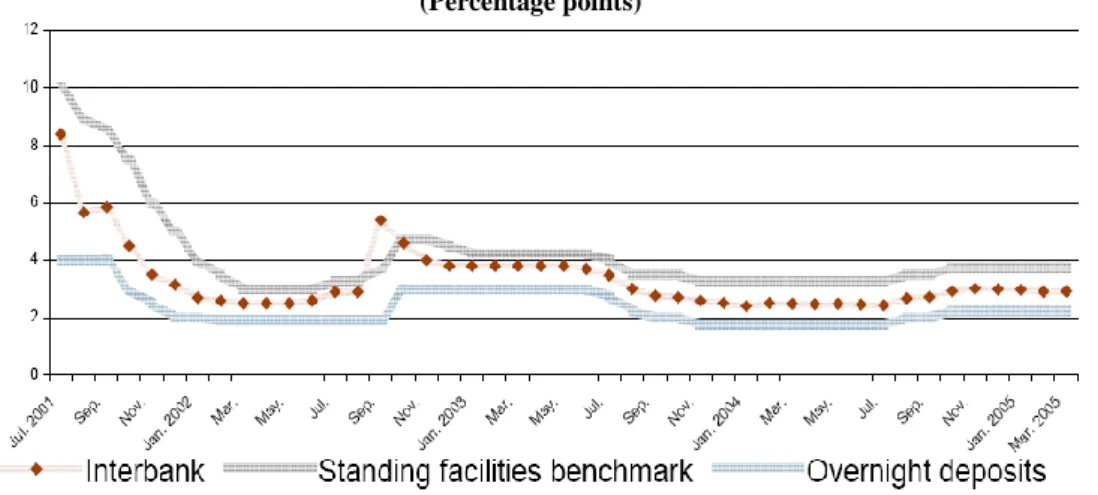
. Finally, since September 2003, the operational target is the interbank interest rate, which the central bank tries to keep in the centre of the benchmark corridor. Figure 5.1 shows the evolution of the interbank interest rate and the benchmark “corridor” since 2001. As can be seen from it, the operational target based on the interbank interest rate has been successfully achieved since its adoption.

Figure 5.1: Interbank, Benchmark (Ceiling), and Overnight Deposits (Floor) Interest Rates.

(Percentage points)

Source: Armas and Grippa (2005).

Based on the above discussion, our empirical analysis considers five samples: April 1995- December 2005 (full sample), April 1995-January 2001 (before the announcement of the benchmark “corridor”), April 1995-December 2001 (before the

environment made communication easier with a monetary target, because the gradual reduction of the base money growth rate was a good indicator of commitment to disinflation. In addition, the high level and variability of expected inflation do not favoured the use of an interest rate operational target: inflation expectations changes would have been a significant noise in the signalling of monetary policy stance. In a low inflation environment, however, monetary targets are less helpful because monetary aggregates tend to be loosely correlated with inflation in the short run. Moreover, it is difficult to communicate the policy stance because changes in the monetary target might be due to expected changes in money demand. In addition, this target does not favour the capital market in domestic currency because the short term interest rate might be too volatile.

33 _{The benchmark “corridor” for the interbank interest rate is a range determined by a “ceiling” and}

“floor” interest rate. The ceiling interest rate for the interbank funds market is given by the benchmark interest rate for injection standing facilities. The “floor” interest rate is given by the overnight deposits interest rate.

adoption of inflation targeting), February 2001-December 2005 and January 2002-December 2005. The data was provided by the Central Bank of Peru and is described in Appendix 1.

5.2. Recursive identification in a standard VAR

As a starting point, we first estimate VARs for the full sample which includes the logs of real GDP (LS004), CPI (LS0027) and nominal exchange rate (LS037); the interbank interest rate (S001); and the 12-months moving average of total reserves

(S002_ma12) and nonborrowed reserves (S003_ma12)34. Each VAR corresponds to a

different specification of the monetary policy indicator: interbank interest rate, nonborrowed reserves and nonborrowed reserves orthogonal to total reserves. The IRFs are displayed in Figures 5.2-5.4.

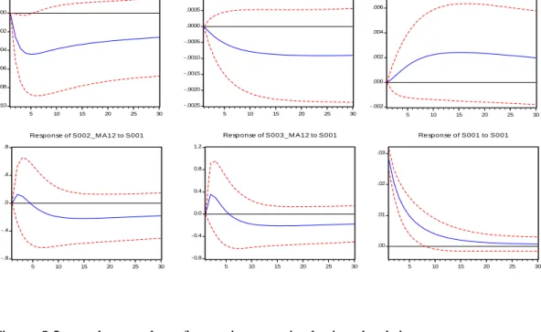
Figure 5.2: IRFs using interbank interest rate as monetary policy indicator (recursive identification)

In Figure 5.2 we observe that after an increase in the interbank interest rate, output and prices decrease as expected, but exchange rate increases. Also, narrow monetary aggregates unexpectedly increase initially, and after five months decrease.

34 _{The results were similar considering 24 and 36 months for the moving average.}

-.010 -.008 -.006 -.004 -.002 .000 .002 5 10 15 20 25 30 Response of LS004 to S001 -.0025 -.0020 -.0015 -.0010 -.0005 .0000 .0005 .0010 5 10 15 20 25 30 Response of LS027 to S001 -.002 .000 .002 .004 .006 5 10 15 20 25 30 Response of LS037 to S001 -.8 -.4 .0 .4 .8 5 10 15 20 25 30 Response of S002_M A12 to S001 -0.8 -0.4 0.0 0.4 0.8 1.2 5 10 15 20 25 30 Response of S003_M A12 to S001 .00 .01 .02 .03 5 10 15 20 25 30 Response of S001 to S001

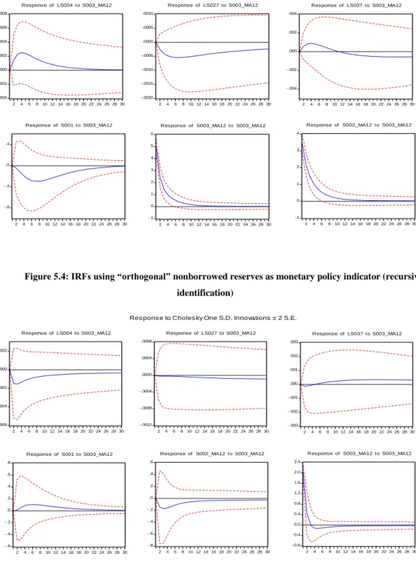
Figure 5.3: IRFs using nonborrowed reserves as monetary policy indicator (recursive identification)

Figure 5.4: IRFs using “orthogonal” nonborrowed reserves as monetary policy indicator (recursive identification)

In the other two cases (figures 5.3 and 5.4), the “assumed” expansionary monetary policy shock displays unexpected movements in output (orthogonal nonborrowed reserves), prices (both cases), exchange rate (orthogonal nonborrowed reserves) and interest rate (orthogonal nonborrowed reserves). Thus, in terms of the IRFs, these baseline results do not provide a good guidance to choose a relevant monetary policy

-.004 -.002 .000 .002 .004 .006 .008 2 4 6 8 10 12 14 16 18 20 22 24 26 28 30 Response of LS004 to S003_MA12 -.0020 -.0015 -.0010 -.0005 .0000 .0005 .0010 2 4 6 8 10 12 14 16 18 20 22 24 26 28 30 Response of LS027 to S003_MA12 -.004 -.002 .000 .002 .004 2 4 6 8 10 12 14 16 18 20 22 24 26 28 30 Response of LS037 to S003_MA12 -.8 -.4 .0 .4 2 4 6 810 12 14 16 18 20 22 24 26 28 30 Response of S001 to S003_MA12 -1 0 1 2 3 4 5 6 2 4 6 8 10 12 14 16 18 20 22 24 26 28 30

Response of S003_MA12 to S003_MA12

-1 0 1 2 3 4 2 4 6 8 10 12 14 16 18 20 22 24 26 28 30

Response of S002_MA12 to S003_MA12

Res pons e to Choles ky One S.D. Innovations ± 2 S.E.

-.006 -.004 -.002 .000 .002 2 4 6 810 12 14 16 18 20 22 24 26 28 30 Response of LS004 to S003_MA12 -.0012 -.0008 -.0004 .0000 .0004 .0008 2 4 6 810 12 14 16 18 20 22 24 26 28 30 Response of LS027 to S003_MA12 -.003 -.002 -.001 .000 .001 .002 .003 2 4 6 810 12 14 16 18 20 22 24 26 28 30 Response of LS037 to S003_MA12 -.6 -.4 -.2 .0 .2 .4 .6 .8 2 4 6 810 12 14 16 18 20 22 24 26 28 30 Response of S001 to S003_MA12 -.8 -.6 -.4 -.2 .0 .2 .4 .6 2 4 6 810 12 14 16 18 20 22 24 26 28 30

Response of S002_MA12 to S003_MA12

-0.8 -0.4 0.0 0.4 0.8 1.2 1.6 2.0 2.4 2 4 6 810 12 14 16 18 20 22 24 26 28 30

Response of S003_MA12 to S003_MA12

indicator as long as they do not mimic the expected effects of the macroeconomic

variables considered35.

5.3. SVAR and the market for bank reserves

Table 1 displays the estimation results for Models 1, 2, 3 and 4 as proposed by Bernanke and Mihov (1998) and the corresponding test of overidentifying restrictions.

The estimates of d, which describes the central bank‟s propensity to accommodate

reserve demand shocks, are around 1 for all subsamples analyzed (Models 3 and 4) and show high statistical significance, implying that the central bank fully accommodates

shocks in reserves demands. This result is inconsistent with Model 2, where d 0.

There is also evidence that the central bank offsets shocks in the reserve market, as long

as b is negative and statistically significant. However, in absolute values, the estimates

of b are much smaller than the estimates of d , which is consistent with the rejection

of Model 1 in all samples.

The estimates of  and  are positive and statistically significant in all samples

(for relevant models), except in the case of Model 2 (nonborrowed reserves) for the samples 2001m2-2005m12 and 2002m1-2005m12. The implied liquidity effect ranges from 25 (Model 1, sample 1995m1-2001m12) to 160 basis points (Model 2, sample 2002m1-2005m12).

Overall, these results show evidence in favour of Model 3 (NBR/TR), and rejects Model 1 (FFR). From Table 1 it can be observed that for all samples, Model 3 (NBR/TR) is not rejected and Model 1 (FFR) is always rejected; and for the last two samples (2001m2-2005m12) Model 2 (NBR) cannot be rejected. However, considering CEE (1999)'s observation about Bernanke and Mihov‟s identification procedure, the

rejection of FFR can be interpreted as a rejection of the implied assumption 0.

Thus, to confirm that Model 3 (NBR/TR) is the best choice with respect to the other models, we need to compare their corresponding impulse-response functions (IRFs) as

35

It is important to mention that analogous results were obtained for different VARs specifications (more and different variables).