Accepted Manuscript
Out-of-Sample Equity Premium Predictability and Sample Split–Invariant Inference
Gueorgui I. Kolev, Rasa Karapandza
PII: S0378-4266(16)30137-6
DOI: 10.1016/j.jbankfin.2016.07.017
Reference: JBF 4995
To appear in: Journal of Banking and Finance
Received date: 11 May 2013 Revised date: 8 July 2016 Accepted date: 11 July 2016
Please cite this article as: Gueorgui I. Kolev, Rasa Karapandza, Out-of-Sample Equity Premium Predictability and Sample Split–Invariant Inference, Journal of Banking and Finance (2016), doi:
10.1016/j.jbankfin.2016.07.017
This is a PDF file of an unedited manuscript that has been accepted for publication. As a service to our customers we are providing this early version of the manuscript. The manuscript will undergo copyediting, typesetting, and review of the resulting proof before it is published in its final form. Please note that during the production process errors may be discovered which could affect the content, and all legal disclaimers that apply to the journal pertain.
ACCEPTED MANUSCRIPT
Out-of-Sample Equity Premium Predictability
and Sample Split–Invariant Inference
G
UEORGUII. K
OLEV†Middlesex University Business School, London, United Kingdom
R
ASAK
ARAPANDZA‡EBS Business School, Wiesbaden, Germany
Abstract
For a comprehensive set of 21 equity premium predictors we find extreme variation in out-of-sample predictability results depending on the choice of the sample split date. To resolve this issue we propose reporting in graphical form the out-of-sample predictability criteria foreverypossible sample split, and two out-of-sample tests that are invariant to the sample split choice. We provide Monte Carlo evidence that our bootstrap-based inference is valid. The in-sample, and the sample split invariant out-of-sample mean and maximum tests that we propose, are in broad agreement. Finally we demonstrate how one can construct sample split invariant out-of-sample predictability tests that simultaneously control for data mining across many variables.
JEL classification:G12, G14, G17, C22, C53
Keywords:equity premium predictability, out-of-sample inference, sample split choice, bootstrap
†Contact Author. Address: Middlesex University Business School, Room W214, London NW4 4BT, United
Kingdom; Office Phone: +44 (0) 208 411 5150, Mobile Phone: +44 (0) 755 197 8531; Email: [email protected]. We would like to thank Ronald W. Anderson, Rene Garcia, Benjamin Golez, and Abraham Lioui as well as two anonymous referees for detailed comments and suggestions. Remaining errors are ours.
‡Address: Department of Finance, Accounting & Real Estate, EBS Business School, Gustav-Stresemann-Ring 3,
ACCEPTED MANUSCRIPT
1. Introduction
The question of whether asset returns are predictable is important not only from the theoretical (asset-pricing) perspective but also from the practical (market-timing) perspective. An important concern is whether in-sample or instead out-of-sample econometric methods should be used to assess the predictability of returns. According to Ashley, Granger, and Schmalensee (1980, p. 1149), “the out-of-sample forecasting performance” provides “the best information” and should therefore be preferred. More recently, Inoue and Kilian (2004) argue that out-of-sample tests are less able to reject a false null hypothesis; that loss of power is due to splitting the finite sample into an in-sample estimation period and an out-of-sample evaluation period, although the authors acknowledge there is a role for out-of-sample methods in choosing the best (though possibly misspecified) forecasting model among the few competitors. Hence most attention in the recent literature on returns predictability has focused on out-of-sample forecasting methods and inference (see, among others, Goyal and Welch, 2003; Rapach and Wohar, 2006; Campbell and Thompson, 2008; Kolev, 2008; Welch and Goyal, 2008; Rapach, Strauss, and Zhou, 2010).1 Out-of-sample methods involve splitting the available data into an in-sample estimation period, which is used to produce an initial set of regression estimates, and an out-of-sample forecast evaluation period over which forecasts are generated and then both evaluated (in terms of some specified criterion of goodness) and compared with results from competing models (West, 2006, p. 106). The natural question that arises in this context is justhowthe sample should be split into these two periods. This paper considers a set of 21 predictors (including those used in the influential paper of Welch and Goyal, 2008). We demonstrate that some such splits yield results indicating that returns arenotpredictable whereas other splits lead to the opposite conclusion. That is: for any given predictor and any given data set, the derived predictability of returns is sensitive to where the sample is split between the estimation and forecast evaluation subsamples.
To address this problem and resolve contradictory findings, we propose two simple (but com-1Apart from equity premium predictability, another interesting and active field of finance addresses whether
mean-variance optimization improves on the naive 1/Nportfolio allocation rule on anout-of-sample basis (DeMiguel, Garlappi, and Uppal, 2009; Kirby and Ostdiek, 2012). The issues we raise as well as our proposed inferential methods are applicable also to this problem—provided the expected portfolio return under the null (e.g., with naive 1/Nportfolio weights) and the expected portfolio return under the alternative (e.g., with mean-variance–optimal weights) can be written as a regression function of the returns of the underlying assets constituting the portfolio. Britten-Jones (1999) shows how mean-variance optimization can be recast as a regression problem.
ACCEPTED MANUSCRIPT
putationally intensive) methods that do not suffer from this dependence on the choice of split date. The first approach is to report in graphical form the out-of-sample predictability results forevery
possible sample split. Thus we report thep-values for the Clark and West (2007) mean squared pre-diction error–adjusted (MSPE-adj) statistic for every possible sample split, where the sample split dateτfalls within the interval[int(.05T),T−int(.05T)]; here int(·)denotes the argument’s integer part. It follows that neither the in-sample estimation period nor the out-of-sample evaluation period ever contains less than 5% of the total numberTof observations. Computationally, we determine thep-value by generating 9999 bootstrap samples under the null of no predictability and then cal-culating thet-statistic associated with the MSPE-adj for eachτ; let us call this witht(MSPE-adj)τ to emphasize that one such statistic goes with each individual sample split indexed byτ. Then thep-value for each sample splitτis the fraction of bootstrap samples for which the bootstrap
t-statistic is larger than thet-statistic calculated from the original data for the correspondingτ. The second approach is to calculate, again across all possible sample splits, some summary statistic of an out-of-sample predictability criterion and then, via a bootstrap procedure, to deter-mine (for inferential purposes) thedistributionof that statistic under the null hypothesis of no return predictability. Thus we calculate meanτ{t(MSPE-adj)τ}and maxτ{t(MSPE-adj)τ}, the mean and the maximum taken overτ. In this way we capture the entire sequence of statistics t(MSPE-adj)τfor eachτ. We evaluate the 15 predictors considered in Welch and Goyal (2008) and six additional, behavioral predictors (that end up failing to predict the equity premium). We show thatsomeof the traditional forecasting variables work very well forsomesample splits. The satisfactory (albeit episodic) performance of traditional predictors is in contrast to the widespread failure of behavioral predictors. The hypothesis that investor sentiment predicts future stock re-turns is a plausible one, and it is not unreasonable to suppose that such sentiment can be measured (howsoever imperfectly) by behavioral factors. Yet of all the behavioral sentiment variables we examine, only one is predictive of the equity premium: Equity Share in New Issues.
We can summarize as follows the issues at hand and our paper’s contributions.
1. Scholars who are interested in such general questions as “Are stock returns predictable?” and who want to use out-of-sample methods should not take the sample split date as given. We propose two methods of dealing with this sample split problem: (i) report the results for each
ACCEPTED MANUSCRIPT
possible sample split; or (ii) calculate a statistic that is invariant to the chosen sample split within any given set of possible sample splits.
2. We document that conclusions about stock market predictability when using out-of-sample methods are strongly dependent on the choice of a sample split date. In fact, a researcher may derive evidence supporting (or refuting) predictability simply by adjusting the sample split date. We also show that traditional predictors of stock returns exhibit satisfactory performance often but not for all sample splits; in contrast, behavioral predictors hardly ever exhibit satisfactory performance.
3. As soon as one allows any possible sample split to be chosen (e.g., via the mean or maximum of results based on various forecasting criteria taken across all possible sample splits), most debates over competing in- or out-of sample methods and splits become moot. Results from using in-sample methods are in broad agreement with those from using sample split–invariant out-of-sample methods.
4. We show how to construct out-of-sample predictability tests that (i) are sample split invariant and (ii) control for data mining. Using this out-of-sample, sample split independent joint test of predictive power of 21 predictors we reject the null hypothesis of no predictability - contrary to results of Welch and Goyal (2008).
5. We provide Monte Carlo evidence to support the validity of our bootstrap-based inference. Four other works are closely related to this paper. Hubrich and West (2010) and Clark and McCracken (2012) propose taking the maxima of various statistics for simultaneously judg-ing whether a small set of alternative models that nest a benchmark model improve upon the benchmark model’s MSPE. After completing this paper, we became aware of independent and contemporaneous work by Rossi and Inoue (2012) and Hansen and Timmermann (2012). Both of these papers examine in great detail the theoretical econometric properties of the sample split problem. Rossi and Inoue derive the theoretical distribution of (general) sample split–invariant mean and maximum tests; Hansen and Timmermann propose a “minimump-value” approach to sample split–invariant inference.
For nested model comparisons, such as our paper’s asset pricing application, Rossi and Inoue (2012) propose taking either the mean or the maximum over all possible sample splits of the
ACCEPTED MANUSCRIPT
Clark and McCracken (2001) ENC-NEW test statistic. Rossi and Inoue characterize and tabulate the distributions of their mean and maximum tests. We show via Monte Carlo experiments that their tabulated null distributions poorly approximate the true null distributions for asset pricing applications such as ours. Take, for example, our Monte Carlo simulation where calibration is based on time-series properties of the dividend-to-price ratio (with 1200 time-series observations). At the 5% nominal significance level, the Rossi and Inoue (2012)meantest statistic has empirical size of 9.81%; similarly, at the 5% nominal significance level theirmaximumtest statistic has empirical size of 13.25%. So for a predictor with the time series properties of the dividend-to-price ratio their test over-reject the true null even for samples as large as 1200 observations.
Hence our paper differs from both Rossi and Inoue (2012) and Hansen and Timmermann (2012) along several dimensions. First, we employ bootstrap techniques so that we can evaluate empiri-cally the null distributions of the mean and maximum tests. Doing so renders our testing procedure robust not only to the nearly nonstationary behavior of the predictors (since the autoregressive parameters of the predictive variables are approximately 1) but also to the high correlation between innovations of the predictive variables and innovations of the predicted term (e.g., returns). Note that those high correlations and also predictor nonstationarity are characteristic of real-world financial data. Second, we evaluate comprehensively the out-of-sample forecasting performance of 21 equity premium predictors; we find that it is possible to predict the equity premium and also show that the distributions of test statistics are not pivotal. Hence, we argue that any sample split independent test based on a theoretical distribution that isnota function of the predictor’s autore-gressive parameter and of the correlation between innovations of predictor and predictand (like those derived by Rossi and Inoue and by Hansen and Timmermann) will not work well in practice. Third, we show that our bootstrap procedure allows one to control for data-mining issues by evaluating thejointforecasting ability of a set of predictive variables. Such control is not feasible under the approaches adopted by Rossi and Inoue (2012) and Hansen and Timmermann (2012).
Several limitations of this study are worth mentioning. First, we study only single predictors; that is, we do not study combinations of them (as in Welch and Goyal, 2008; Rapach, Strauss, and Zhou, 2010), including combinations based on principal components (e.g., Neely, Rapach, Tu, and Zhou, 2014). Neither do we follow Welch and Goyal by looking at rolling regressions.
ACCEPTED MANUSCRIPT
Also, recent research indicates that the accuracy of traditional predictors (e.g., ratio of dividend to price) can be improved by enlarging the predictive information set with the information implied by derivative markets (Binsbergen, Hueskes, Koijen, and Vrugt, 2011; Golez, 2014; Kostakis, Panigirtzoglou, and Skiadopoulos, 2011). To keep the number of variables that we study tractable we do not include these refinements in our study. Finally, we limit ourselves to standard ordinary least-squares (OLS) regressions that incorporate neither the economic gains nor the utility gains of potential investors. All these extensions should be tractable when pursued within the framework described here, and they constitute a fruitful research agenda.
2. Methodology and data
Following much of the extant literature, we estimate OLS bivariate predictive regressions. In particular, we regress the equity premium—constructed as the return on the S&P 500 index (including dividends distributions) minus the risk-free rate,Rt≡(Rm−Rf)t—on a constant and on a lagged value of a predictor
Rt=β0+β1Xt−1+ut. (1) The predictor X is one of the variables listed in Table 1 (in Section 2.5), depending on the specification. Theβs are population parameters (to be estimated), anduis a disturbance term.
2.1. In-sample predictability
The in-sample predictive ability ofXis assessed via thet-statistic corresponding tob1, the OLS
estimate ofβ1in equation (1). Under the null hypothesis thatXt−1is uncorrelated withRt, the expected returns are constant andβ1=0 (the sign ofβ1is typically suggested by theory). The
tables presented in this paper are agnostic concerning whether the alternative hypothesis is one-or two-sided and simply repone-ortt-statistics associated with the estimates. The estimated slopes for all variables are in the direction predicted by theory and so, roughly speaking, one can consider a
t-statistic whose absolute value exceeds 1.65 to be significant either at the 10% significance level for the two-sided alternative or at the 5% significance level for the one-sided alternative.
cor-ACCEPTED MANUSCRIPT
related with those in the predictand, severe small-sample biases may occur (Mankiw and Shapiro, 1986; Stambaugh, 1986; Nelson and Kim, 1993; Stambaugh, 1999). To test whether the in-sample
results could be an artifact of this small-sample bias, we follow the bias correction methodology of Amihud and Hurvich (2004). The model is defined over the whole samplet=1,2,...,T,
Rt=β0+β1Xt−1+ut, (2)
Xt=µ+ρXt−1+wt; (3) where the disturbances(ut,wt)are serially independently and identically distributed as bivariate normal, and the autoregressive coefficient in equation (3) is less than 1.
We shall use superscriptcto denote a bias-corrected estimator. First, we estimate equation (3) to obtain the OLS estimatorrofρ. We can then userto compute the bias-corrected estimator ofρas follows:
rc=r+1+3r
T +
3(1+3r)
T2 . (4)
This bias-corrected estimatorrcis, in turn, used to compute the corrected residuals ˆwc
t of equa-tion (3):
ˆ
wct=Xt−(m+rcXt−1),
wheremis the OLS estimator ofµ.2
Next, we run an auxiliary regression of Rt on an intercept, Xt−1 and ˆwct. In this auxiliary regression, letbc1(resp., fc) be the OLS estimator of the slope parameter onXt−1(resp., on ˆwtc). Herebc1is the bias-corrected estimator ofβ1, our variable of interest.
Finally, to conduct inferences based onβ1we need the bias-correctedstandard error(SE) of
bc
1, which is given by
[SEc(bc1)]2= [fc]2∗[1+3/T+9/T2]2∗[SE(r)]2+[SE(bc1)]2, (5) where SE(r)denotes the usual OLS standard error ofrproduced by any regression package and SE(bc
1)denotes the usual OLS standard error ofbc1, which comes as a direct output from the
ACCEPTED MANUSCRIPT
auxiliary regression ofRton an intercept,Xt−1and ˆwct.
2.2. Out-of-sample predictability: Fixed sample split date
We generate out-of-sample predictions by the following recursive scheme. First we split the available sample into an in-sample estimation period and an out-of-sample evaluation period. Let
T denote the total number of observations and let dates run from 1 toT inclusive. As described in the Introduction, we fix a dateτ∈[int(.05T),T−int(.05T)]. We use the first period,[1,τ−1], for the in-sample estimation and use the second period,[τ,T], for making out-of-sample predictions.
For timet, we useRpn,t=b0,t−1to denote the null model prediction andRpa,t=b0,t−1+b1,t−1Xt−1
to denote the alternative model prediction. Here “pn” stands for “prediction with the null imposed” (i.e., whenb1is constrained to be 0), and “pa” stands for “prediction under the alternative” (i.e.,
using equation (1)).
Theb-values are estimated by OLS using data no more recent than one periodbeforethe forecast is made. Thus the first prediction under equation (1) isRpa,τ=b0,τ−1+b1,τ−1Xτ−1, where each
bis estimated using only data points fromt=1 throught=τ−1. The second prediction is
Rpa,τ+1=b0,τ+b1,τXτ, where theb-values are estimated using only data points from the 1st period though theτth period. The last prediction isRpa,T=b0,T−1+b1,T−1XT−1; here eachbis
estimated using only data points from period 1 though periodT−1.
In this way we obtain, for each fixedτ, a sequence of predictions under the null model and also a sequence of predictions under the alternative model. As an informal measure of the predictive regression’s out-of-sample performance, we calculate the out-of-sample R-squared of Campbell and Thompson (2008):
R2os(τ) =1−∑t=τ,...,T(Rt−Rpa,t)
2
∑t=τ,...,T(Rt−Rpn,t)2 (6)
(here “os” stands for “out-of-sample”).
We formally test the null hypothesis—that equation (1) doesnotimprove on the historical average return—by employing the Clark and West (2007) mean squared prediction error–adjusted
ACCEPTED MANUSCRIPT
statistic: MSPE-adj(τ) =∑t=τ,...,T{(Rt−Rpn,t) 2−[(R t−Rpa,t)2−(Rpn,t−Rpa,t)2]} ∑t=τ,...,T1 . (7)Clark and West (2007) observe that under the null thatβ1=0, the alternative model in eq. (1)
estimates additional parameters whose population values are 0, and that the estimation induces additional noise. Hence under the null hypothesis the MSPE of the alternative model is expected to be larger than the null model’s. These authors propose an adjustment to the alternative model’s MSPE. In equation (7), the term in brackets is theadjustedMSPE of the alternative model. We calculate thet-statistic associated with equation (7); following Clark and West, we denote it t(MSPE-adj)τ. We regress the quantity in braces in equation (7) on a constant; thet-statistic from this regression,t(MSPE-adj)τ, is calculated for each sample splitτ.
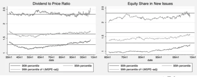
Clark and West (2007, p. 298) justify the approximate normality of their t(MSPE-adj)τ statistic by observing that its null distribution obeys the following inequalities across a large set of simulations: (90th percentile) ≤ 1.282 ≤ (95th percentile); and (95th percentile) ≤ 1.645 ≤ (99th percentile). In these expressions, the percentiles refer to the distribution of thet(MSPE-adj)τ statistic under the null of no predictability (i.e., thet-ratio associated with MSPE-adj). Indeed, these inequalities are usually satisfied in our bootstrap simulations. Figure 1 (left) shows the predictor for which the previous inequalities aremostoften violated, which is the dividend-to-price ratio. This figure plots the 90th, 95th and 99th percentiles of the bootstrap null distribution oft(MSPE-adj)τfor each sample split dateτ; the horizontal lines at 1.2815, 1.6448, and 2.3263 mark the respective percentiles in the standard normal distribution. All violations of these inequalities are slight, so is reasonable to infer that predictability is approximately normal. More troublesome is that, for the other predictive variables, the corresponding plots look like Figure 1 (right, for the Equity Share in New Issues’ predictor).3 For these 20 predictors, the
inequalities in Clark and West (2007, p. 298) are satisfied yet the approximately normal inference is usually too conservative. In particular: for most of the sample splitsτand most of the predictive variables, the 90th percentile of the bootstrap null distribution oft(MSPE-adj)τ is slightly less than 1—instead of about 1.282 (the 90th percentile in the standard normal distribution).
ACCEPTED MANUSCRIPT
Figure 1: Plots of the 90th, 95th, and 99th percentiles of the null distribution oft(MSPE-adj)τ statistic versusτ (the start of the out-of-sample forecasting exercise), together with straight horizontal lines at 1.2815, 1.6448 and 2.3263 that mark the respective percentiles in the standard normal distribution, when the Dividend to Price Ratio (left) and the Equity Share in New Issues (right) are used as a predictor of the Equity Premium.
We therefore eschew the normal approximation of Clark and West (2007) and instead use bootstrapping to calculate thet(MSPE-adj)τ statistic’sp-value at each sample split. Thep-value fort(MSPE-adj)τ, which we shall denote pv(τ), is calculated by drawing 9999 bootstrap samples under the null hypothesis of no predictability and, for each draw, calculatingt(MSPE-adj)τ. Then pv(τ)is the fraction of times that this statistic calculated from the null distribution bootstrap sample is greater than the same statistic calculated from the original data.
After calculatingR2
os(τ)and pv(τ)for each possible sample split dateτ, we can construct a
graph that plots those two calculated terms againstτ. This graph contains all the information needed to assess how well an investor making decisions in real time would have done, on an out-of-sample basis, by using the predictor in question starting at sample split dateτ.
2.3. Out-of-sample predictability: Invariant to sample split date
If the aim is to distill into a single indicator whether the equity premium is predictable on an out-of-sample basis, then one can construct a summary statistic of the distribution oft(MSPE-adj)τ across the sample split datesτ. For instance, Roy’s (1953) union-intersection principle dictates that we donotreject the null of no predictability if none of thet(MSPE-adj)τ statistics reject it. We shall therefore reject that null only if at least one of thet(MSPE-adj)τrejects the null for at
ACCEPTED MANUSCRIPT
least oneτ. Formally, that approach is equivalent to using
maxτ{t(MSPE-adj)τ} (8) as a test statistic; alternatively, we could use
meanτ{t(MSPE-adj)τ} (9)
as a test statistic.
There is no clear basis ex ante for preferring one of equations (8) and (9) over the other, since the null distribution is not known for either test statistic. Hence we determine the null distribution of both the maximum and the mean statistics just displayed by generating 9999 bootstrap samples under the null of no predictability. After computing the two statistics for each of these bootstrap samples, we calculate the p-value of the maximum (resp. mean) test statistic by counting how often the bootstrap maximum (resp. mean) statistic is larger than the maximum (resp. mean) statistic calculated from the original data. As before, the bootstrap samples are generated while imposing the null hypothesis of no predictability.
2.4. Bootstrap procedure: Description
To generate our 9999 bootstrap samples under the null hypothesis of no predictability, we follow Mark (1995), Kilian (1999), Rapach and Wohar (2006), and Welch and Goyal (2008). (For a general treatment of bootstrap hypothesis testing, see MacKinnon, 2009—especially its section on the residual bootstrap.) We use the original data to estimate equations (2) and (3) by ordinary least squares and then store the residuals ( ˆutand ˆwt) for resampling.4Next we use the original data to estimate equations (2) and (3) via OLS while imposing the null hypothesis of no predictability (β1=0); the resulting restricted estimates are denoted ˜β0, ˆµ, and ˆρand are stored for later use
to generate bootstrap data under the null.
4Rapach and Wohar (2006, p. 237) resample the restricted model residuals (i.e., the residuals whenβ
1=0); Welch
and Goyal (2008, p. 1462) resample the unrestricted residuals. According to MacKinnon (2009, p. 195), “there might be a slight advantage in terms of power if we were to use unrestricted rather than restricted residuals.” We therefore opt to resample the unrestricted residuals.
ACCEPTED MANUSCRIPT
The sample is restricted in thatXt is available only for timest=0,...,T andRt is available only for timest=1,...,T. To initiate the recursion in equation (3), we randomize (with equal probability) over datest=0,...,T, denote the drawt0, and setX0b=Xt0. Then we randomize again with equal probability but now with replacement over datest=1,...,T; we uset∗to signify a
single draw from this randomization. For one bootstrap round we generateT such draws. Then we setub
t =uˆt∗ andwtb=wˆt∗fort=1,...,T, thereby drawing (with replacement) the residuals ˆut
and ˆwtas a pair that are matched bytto preserve their cross correlation. For each bootstrap round, we generateRb
t =β˜0+ubt andXtb=µˆ+ρˆXtb−1+wtbfort=1,...,T. Finally, the 9999 bootstrap samples generated under the null of no predictability are obtained by following the same procedure another 9999 times. We estimate the unrestricted model in equations (2) and (3) for each of the 9999 bootstrap-generated data sets onRtband onXtband then calculate, for each set, the statistics described previously:R2os(τ)and t(MSPE-adj)τ for each τ as well as maxτ{t(MSPE-adj)τ} and meanτ{t(MSPE-adj)τ}. These 9999 replicates of each are used to estimate each statis-tic’s distribution under the null hypothesis of no predictability. For example, we evaluate the
p-value of the maximum statistic by checking for how many of the 9999 bootstrap samples maxτ{t(MSPE-adj)τ}is larger than maxτ{t(MSPE-adj)τ}calculated for the original data.
2.5. Data
The equity premium measure that we use,Rt≡(Rm−Rf)t, is based on monthly returns on the S&P 500 index, including dividends. The end-of-month values are a series provided by the Center for Research in Security Prices for the period January 1926 to December 2010; we subtract the risk-free rate, defined as the contemporaneous 1-month US Treasury bill (T-bill) rate.
We study the predictive performance of 21 variables. Of these, the first 15 are from Welch and Goyal (2008) and are downloaded from Amit Goyal’s website. The remaining six arebehavioral
predictors; they are downloaded from Jeffrey Wurgler’s Web page.
ACCEPTED MANUSCRIPT
Table 1: Summary statistics.
Variable Mean Std. Dev. Min. Max. T
Equity Premuim, (Rm - Rf) 0.0062 0.0559 -0.2877 0.4162 1020
Variables downloaded from Amit Goyal’s web site
Dividend to Price Ratio -3.3239 0.4511 -4.524 -1.8732 1021
Dividend Yield -3.3197 0.4494 -4.5313 -1.9129 1020
Book to Market Ratio 0.5868 0.2654 0.1205 2.0285 1021
Earnings to Price Ratio -2.7141 0.4255 -4.8365 -1.775 1021
Dividend Payout Ratio -0.6097 0.3229 -1.2247 1.3795 1021
Treasury Bill Rate 0.0366 0.0306 0.0001 0.163 1021
Long Term Yield 0.053 0.028 0.0182 0.1482 1021
Long Term Return 0.0047 0.0239 -0.1124 0.1523 1020
Term Spread 0.0163 0.0131 -0.0365 0.0455 1021
Default Yield Spread 0.0114 0.0071 0.0032 0.0564 1021
Default Return Spread 0.0003 0.0132 -0.0975 0.0737 1020
Inflation Lagged 2 Months 0.0024 0.0053 -0.0208 0.0574 1021
Net Equity Expansion 0.0191 0.0246 -0.0575 0.1732 1009
Stock Variance 0.0025 0.005 0.0001 0.0558 1021
Cross Sectional Premium 0.0004 0.0024 -0.0042 0.0077 788
Variables downloaded from Jeffrey Wurgler’s web site
Dividend Premium -2.2399 16.2884 -50.23 32.9 600
Number of IPOs 26.2516 23.6031 0 122 612
Average First-day IPO Returns 16.3867 20.0237 -28.8 119.1 612
NYSE Share Turnover 0.5084 0.3665 0.105 1.738 636
Closed-end Fund Discount 8.9577 7.4353 -10.91 25.28 548
Equity Share in New Issues 0.1827 0.1092 0.0167 0.6349 636
3. Results
3.1. In-sample predictability
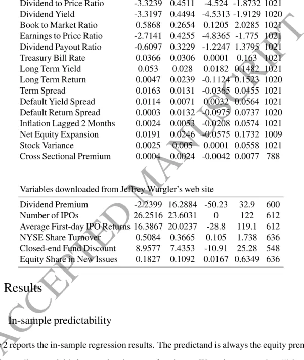
Table 2 reports the in-sample regression results. The predictand is always the equity premium, and the predictor variable is named at the start of each row. We estimate equation (1) by OLS; theb1value, thet-statistic for that value, and the R-squared from estimating equation (1) are
given in (respectively) the first, second, and third data columns of the table. The fourth column reports the bias-corrected estimatorbc
1ofβ1from the predictive regression,
ACCEPTED MANUSCRIPT
thetc-statistic(=bc
1/[SEc(bc1)]). The values in the sixth column are forr, the OLS estimate of
the autoregressive parameterρin equation (3); the seventh column givesrc, the bias-corrected estimator ofρ. The table’s last column reports f, an unbiased estimator of[Cov(ut,wt)]/[Var(wt)] (Amihud and Hurvich, 2004, Lemma 1).
Table 2: In-sample predictive regressions estimates, and bias corrected in-sample estimates.
b1 t-stat R-sq bc1 tc-stat r rc Cov(ut,wt)/Varwt
Dividend to Price Ratio 0.0087 2.26 0.0050 0.0050 1.28 0.99 1.00 -0.96
Dividend Yield 0.0101 2.59 0.0066 0.0098 2.51 0.99 1.00 -0.08
Book to Market Ratio 0.0196 2.98 0.0087 0.0157 2.38 0.98 0.99 -1.01
Earnings to Price Ratio 0.0088 2.13 0.0044 0.0063 1.54 0.99 0.99 -0.62
Dividend Payout Ratio 0.0018 0.34 0.0001 0.0015 0.28 0.99 1.00 -0.08
Treasury Bill Rate -0.0966 -1.69 0.0028 -0.1011 -1.77 0.99 1.00 -1.14
Long Term Yield -0.0750 -1.20 0.0014 -0.0862 -1.38 1.00 1.00 -2.86
Long Term Return 0.1153 1.57 0.0024 0.1155 1.57 0.04 0.04 0.25
Term Spread 0.1823 1.37 0.0018 0.1823 1.37 0.96 0.96 0.01
Default Yield Spread 0.4105 1.67 0.0027 0.3733 1.52 0.98 0.98 -9.67
Default Return Spread 0.1378 1.03 0.0011 0.1382 1.04 -0.12 -0.12 0.57
Inflation Lagged 2 Months -0.3491 -1.06 0.0011 -0.3503 -1.07 0.55 0.55 -0.46
Net Equity Expansion -0.1455 -2.03 0.0041 -0.1461 -2.04 0.97 0.98 -0.16
Stock Variance -0.2039 -0.58 0.0003 -0.2142 -0.61 0.62 0.63 -3.65
Cross Sectional Premium 2.1014 3.03 0.0115 2.0595 2.96 0.98 0.98 -3.44
Dividend Premium 0.0000 0.07 0.0000 -0.0000 -0.17 0.98 0.99 -0.00
Number of IPOs -0.0000 -0.38 0.0002 -0.0000 -0.35 0.86 0.87 0.00
Average First-day IPO Returns 0.0000 0.33 0.0002 0.0000 0.36 0.67 0.68 0.00
NYSE Share Turnover -0.0022 -0.46 0.0003 -0.0023 -0.48 0.97 0.98 -0.02
Closed-end Fund Discount 0.0001 0.20 0.0001 0.0001 0.26 0.96 0.97 0.00
Equity Share in New Issues -0.0402 -2.58 0.0104 -0.0404 -2.59 0.69 0.69 -0.02
An examination of Table 2 reveals that, even after bias correction, many variables remain significant in-sample predictors of the equity premium. At the same time, not even a liberal cut-off point for “significant” (e.g., 1.28) and carrying out a one-sided test at the 10% level are enough to make the following variables significantly predictive: Dividend Payout Ratio, Default Return Spread, Inflation Lagged 2 Months, Stock Variance, Dividend Premium, Number of IPOs, Average First-day IPO Returns, NYSE Share Turnover, and Closed-end Fund Discount.
Predictors that appear to be significant at better than the 5% level (i.e., even when we consider the test to be two-sided) are Dividend Yield, Book to Market Ratio, Net Equity Expansion, Cross Sectional Premium, and Equity Share in New Issues; all of these variables have bias-corrected
ACCEPTED MANUSCRIPT
t-statistics greater than 2 in absolute value (fifth column of Table 2). With the lone exception of Equity Share in New Issues, all of the predictors that have a bias-adjustedt-statistic greater than 2 also have an autoregressive root greater than 0.97—that is, fairly close to 1. Curiously enough, the bias corrections make a big difference only for Dividend to Price Ratio and Earnings to Price Ratio and matter somewhat for Book to Market Ratio; note that these three are exactly the variables by which such corrections were motivated in the first place. The bias correction has little effect on the other 18 predictors.
The behavioral variables—Dividend Premium, Number of IPOs, Average First-day IPO Returns, NYSE Share Turnover and Closed-end Fund Discount —are not statistically significant predictors of the equity premium when judged by the in-sample criterion (with or without bias corrections).
Overall, we have evidence that a large number of variables are statistically significant predictors of the equity premium, even after bias corrections are applied.
3.2. Out-of-sample inference about predictability: Invariant to sample split date
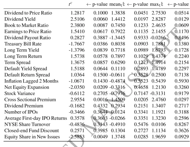
Table 3 presents, side by side, the in-sample results and the out-of-sample (split sample–invariant) results on predictability. Column [1] gives the bias-corrected in-samplet-statistic, and column [2] gives the probability that a standard normal variable is larger than the absolute value of that tc-statistic. Column [3] reports meanτ{t(MSPE-adj)τ}, where the mean is computed overτ; column [4] gives the bootstrap-determined p-value of thepreviouscolumn’s statistic. Analogously, column [5] reports maxτ{t(MSPE-adj)τ}with the maximum taken over τ; its bootstrap-determinedp-value is given in column [6].
The following observations can be made about the results reported in Table 3.
• Noneof the variables that are in-sample insignificant at the 10% level are significant at the 10% level in the two out-of-sample tests. Results of the in-sample bias-corrected test and of
the out-of-sample, sample split–invariant tests are in broad agreement.
• All but one of the predictors appear to be somewhat “less significant” when judged by the two out-of-sample tests.5
ACCEPTED MANUSCRIPT
Table 3: The in-sample bias corrected t-statistic (column 1) is followed by its p-value (column 2). The out-of-sample sample split invariant meanτt(MSPE−adj)τ (column 3) is followed by its bootstrap determined p-value (column 4). The out-of-sample sample split invariant maxτt(MSPE−adj)τ (column 5) is followed by its bootstrap determined p-value (column 6).
tc ←p-value meanτt ←p-value maxτt ←p-value
Dividend to Price Ratio 1.2817 0.1000 1.3838 0.0451 2.7530 0.0514
Dividend Yield 2.5106 0.0060 1.4412 0.0197 2.8287 0.0129
Book to Market Ratio 2.3800 0.0087 0.7450 0.1233 2.4635 0.0609
Earnings to Price Ratio 1.5410 0.0617 0.7922 0.1135 2.1455 0.1170
Dividend Payout Ratio 0.2827 0.3887 -1.3445 0.9333 -0.0266 0.8496
Treasury Bill Rate -1.7667 0.0386 0.8038 0.0903 1.7881 0.1380
Long Term Yield -1.3796 0.0839 0.7718 0.0989 1.6793 0.1728
Long Term Return 1.5738 0.0578 0.7897 0.1029 1.4374 0.2240
Term Spread 1.3675 0.0857 0.6290 0.1273 1.4914 0.2154
Default Yield Spread 1.5188 0.0644 0.1110 0.2893 1.4789 0.2297
Default Return Spread 1.0364 0.1500 -0.0611 0.3528 0.2500 0.7138
Inflation Lagged 2 Months -1.0671 0.1430 -0.4874 0.5523 0.5439 0.5930
Net Equity Expansion -2.0350 0.0209 -0.3316 0.4658 1.2130 0.3260
Stock Variance -0.6112 0.2705 -0.7976 0.7147 -0.3131 0.9179
Cross Sectional Premium 2.9554 0.0016 1.4509 0.0205 2.4760 0.0297
Dividend Premium -0.1682 0.4332 0.2934 0.2151 1.3407 0.2717
Number of IPOs -0.3466 0.3644 0.0124 0.3341 1.1921 0.3188
Average First-day IPO Returns 0.3578 0.3603 -0.0266 0.3351 1.3230 0.2596
NYSE Share Turnover -0.4836 0.3143 -0.4910 0.5476 0.0106 0.8267
Closed-end Fund Discount 0.2571 0.3985 0.1304 0.2727 1.1134 0.3626
Equity Share in New Issues -2.5853 0.0049 1.3748 0.0285 1.9659 0.0929
• Dividend to Price Ratio is the only variable that appears “more significant” when judged by the two out-of-sample criteria than by the in-sample criterion.
• The two out-of-sample criteria agree in a rough sense. In particular, theirp-values are usually within a multiple of 2.
• There are five variables for which the in-sample bias-correctedt-statistic exceeds 2 in absolute value (fifth column of Table 2): Dividend Yield, Book to Market Ratio, Net Equity Expansion, Cross Sectional Premium, and Equity Share in New Issues. Of these, only Net Equity Expansion is insignificant out-of-sample. Each of the other four variables is significant at the 5% level by at least one of the two out-of-sample criteria.
follows that such modifiers as “less” or “more” or “very” (in)significant are, strictly speaking, abuses of statistical terminology. Such wording serves as shorthand for a longer statement; for example, a claim that some predictor is “less significant” judged by test X than by test Y is supposed to mean that if the null hypothesis were true, the probability of observing as large or larger Y as actually observed is smaller than the probability of observing as large or larger X as actually observed.
ACCEPTED MANUSCRIPT
• Every variable shown to be “very insignificant” in-sample (here, having the in-sample bias-correctedt-statistic’sp-value exceed 15%) is shown to be “even more insignificant” by the two out-of-sample statistics (i.e., thep-values for the two out-of-sample statistics exceed 30%). Overall, we do not find much disagreement between in-sample and out-of-sample predictability criteria—provided the latter are invariant to the choice of sample split date. The bias-corrected in-samplet-test as well as the mean and the maximum out-of-sample tests all tell much the same story as regards whether the equity premium is or is not reliably predicted by a given variable.
3.3. Bootstrap null distribution: Selected percentiles of mean and maximum
statistics
For our proposed out-of-sample meanτ{t(MSPE-adj)τ} and maxτ{t(MSPE-adj)τ} sample split–invariant tests, p-values are a function of the test statistic’s observed value and also of its bootstrap determined null distribution. As a result, Table 3 is not informative regarding the distributions of the mean and maximum statistics under the null hypothesis of no predictability. Yet we are interested in such questions as: What do the null distributions of these two statistics look like? Are the mean and maximum statistics pivotal, or do they depend on the parameters of the (bootstrap) data-generating process?
Suppose we found a single null distribution for the mean statistic across all 21 predictors and also a single null distribution for the maximum statistic across those same predictors. In that case, our proposed statistics would be pivotal and independent of the parameters used to generate the data. If, on the contrary, we found the null distributions to be considerably different across the 21 predictors, the implication would be that the two statistics are not pivotal and soaresensitive to those data-generating parameters.
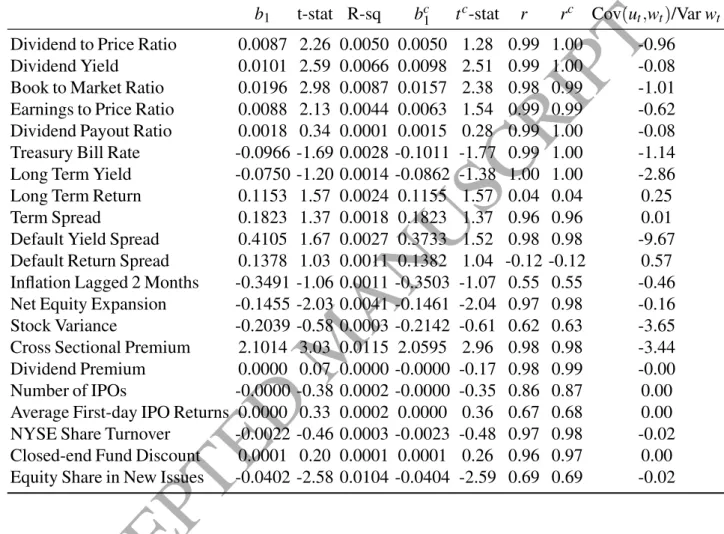
Table 4 reports the 90th, 95th, and 99th percentiles of the bootstrap determined null distribution of the mean and maximum statistics. We can make the following remarks regarding the null distributions of the sample split–invariant meanτ{t(MSPE-adj)τ}and maxτ{t(MSPE-adj)τ} statistics reported in that table.
It seems reasonable to suppose that the meanτ{t(MSPE-adj)τ}and maxτ{t(MSPE-adj)τ} statistics are pivotal because their null distributions do not depend strongly on the parameters of the
ACCEPTED MANUSCRIPT
Table 4: The 90th, 95th, and the 99th percentiles of the bootstrap null distribution for our meanτ[t(MSPE−adj)τ]and maxτ[t(MSPE−adj)τ]sample split invariant statistics, together with the OLS estimate ˆρof the autoregressive parameter in eq.(3) and the correlation between the residuals in eq.(2) and eq.(3).
meant90 meant95 meant99 maxt90 maxt95 maxt99 ˆρ Corr(uˆt,wˆt)
Dividend to Price Ratio 1.0194 1.3464 1.9006 2.4700 2.7584 3.3726 0.99 -0.98
Dividend Yield 0.7398 1.0694 1.7019 1.9404 2.2846 2.9325 0.99 -0.08
Book to Market Ratio 0.8566 1.2002 1.8243 2.2068 2.5456 3.1729 0.98 -0.83
Earnings to Price Ratio 0.8513 1.1801 1.7814 2.2284 2.5810 3.1719 0.99 -0.84
Dividend Payout Ratio 0.7748 1.1038 1.7740 2.0050 2.3316 2.9493 0.99 -0.01
Treasury Bill Rate 0.7506 1.0681 1.7385 1.9486 2.3087 2.9246 0.99 -0.03
Long Term Yield 0.7632 1.1166 1.7847 2.0014 2.3532 3.0198 0.98 -0.12
Long Term Return 0.8055 1.1507 1.7940 1.8994 2.2129 2.7914 0.04 0.13
Term Spread 0.7614 1.0887 1.7607 1.9315 2.2600 2.8933 0.96 -0.04
Default Yield Spread 0.7615 1.1121 1.7419 1.9691 2.2842 2.8938 0.98 -0.25
Default Return Spread 0.7815 1.1261 1.7596 1.9044 2.2201 2.8275 -0.15 0.11
Inflation Lagged 2 Months 0.8093 1.1607 1.7556 1.9101 2.2208 2.8156 0.52 -0.03
Net Equity Expansion 0.7761 1.1037 1.7784 1.9469 2.3134 2.9186 0.97 -0.06
Stock Variance 0.8330 1.1597 1.7575 1.9730 2.2711 2.8478 0.60 -0.36
Cross Sectional Premium 0.7797 1.0876 1.7025 1.9584 2.2737 2.8716 0.98 -0.03
Dividend Premium 0.7507 1.0860 1.7068 1.9992 2.3322 2.9943 0.96 -0.27
Number of IPOs 0.7866 1.1126 1.7594 1.9368 2.2736 2.9246 0.89 0.09
Average First-day IPO Returns 0.8000 1.1293 1.7643 1.9031 2.2460 2.8650 0.61 0.15
NYSE Share Turnover 0.7674 1.1086 1.7464 1.9773 2.3083 2.9197 0.96 -0.02
Closed-end Fund Discount 0.7598 1.1011 1.7463 1.9704 2.2945 2.9526 0.97 0.13
Equity Share in New Issues 0.8175 1.1506 1.7459 1.9185 2.2423 2.8515 0.63 -0.07
bootstrap data-generating process. The percentiles under the null hypothesis of no predictability across the 21 focal predictors are similar, and they are not more dissimilar across predictive variables than are the percentiles of t(MSPE-adj)τ. Under conditional homoskedasticity, t(MSPE-adj)τis known to be pivotal with respect to the parameters of the data-generating process and for the type of forecasting regressions considered here (Clark and McCracken, 2001).6
However, the bootstrap distributions generated under the null of no predictability depend to some extent on the correlation between the error term in equation (2) and that in equation (3). More specifically: the higher the correlation, the higher the percentiles of the null distribution for the
6The null distribution of thet(MSPE-adj)
τstatistic does depend on the constant to which the ratio of evaluation
data points to estimation data points converges as the sample size grows to infinity. The assumption that this ratio is constant is not supported by our calculations for each possible sample split. Of course, statistical behavior as the sample size approaches infinity is an abstraction with no clear meaning in practice; our sample is always finite. Hence the only question is whether or not this abstraction yields an accurate approximation for the samples that are typically available.
ACCEPTED MANUSCRIPT
corresponding predictor. Thus the previous point’s conjecture might just as well turn out to be false. If we are comfortable (for exploratory purposes) with the rough sense in whicht(MSPE-adj)τis approximately normal for a fixed sample split, then we can propose the following rough criterion: if the data-based meanτ{t(MSPE-adj)τ}is greater than 1 (resp., 1.5, 2), then the bootstrap sample split–invariant test would likely reject the null of no predictability at the 10% (resp., 5%, 1%) level of significance. Similarly, we can say that if the data-based maxτ{t(MSPE-adj)τ}is greater than 2 (resp., 2.5, 3) then the sample split–invariant bootstrap test would probably reject the null of no predictability at the 10% (resp., 5%, 1%) level of significance. Even a rule of this approximate nature could save some programming and simulation time, though it must be used with an eye toward the in-sample results. From Table 3 we see that the in-sample test of predictability for a given variable is extremely informative about the complete out-of-sample simulation outcomes.
3.4. Summarizing out-of-sample predictability in graphical form
Figure 2 displays complete information on a real-time investor’s investment outcomes as a function of the sample split. Each sub-figure within Figure 2 presents the out-of-sample R-squared and the bootstrap-determined p-value for the MSPE-adjt-statistic for each sample split date
τ∈[int(.05T),T−int(.05T)]. For eachτwe bootstrap thet(MSPE-adj)τ statistic, rather than the MSPE-adj(τ) statistic, because the former is pivotal and the latter is not. MacKinnon (2009) emphasizes that one should bootstrap pivotal quantities whenever possible because doing so yields an asymptotic refinement: the error in rejection probability committed by the pivot-based
bootstraptest is of lower order in the sample size than is the error in rejection probability of the
asymptotictest based on the same pivot (Beran, 1988; Hall, 1992).
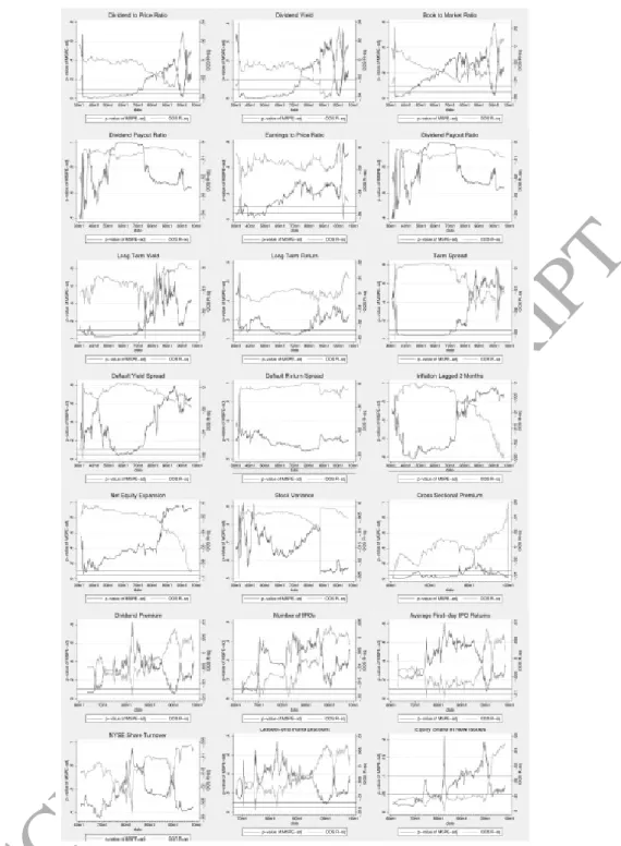
The 21 sub-figures show how well an investor (starting in, say, January 2000; the actual years plotted vary depending on data availability) would have done by using each of our 21 focal predictors—as compared with using the recursive mean—to forecast the equity premium out-of-sample. The following list offers brief comments about the out-of-sample predictive success of each variable as a function of the sample split dateτ. (When discussingoverallin-sample and sam-ple split–invariant out-of-samsam-ple inference about predictability, we refer always to the results in Table 3. We discuss the predictors in Figure 2 consecutively from left to right, and down Figure 2.)
ACCEPTED MANUSCRIPT
Figure 2: Plots of the p-value of thet(MSPE-adj) statistic and the out-of-sample R-squared versusτ(the start of the out-of-sample forecasting exercise).
The (log of the)Dividend to Price Ratiois a reasonably accurate out-of-sample predictor of the equity premium. It loses predictive power around year 1973, but it regains power in the late 1990s and at the start of the new millennium. Then, from about year 2002, it is once again unable to outperform the recursive mean. The sample split–invariant mean and maximum tests show that the dividend-to-price ratio outperforms the recursive mean overall. This is theonlyvariable for which
ACCEPTED MANUSCRIPT
our out-of-sample tests reject the null of no predictability at better significance levels than does the in-sample test. The out-of-sample R-squared is negative for the most part; it becomes positive only for a short period around year 2000. The (log of the)Dividend Yielddisplays the same predictive pattern as Dividend to Price Ratio. All tests—in-sample and sample split–invariant out-of-sample—show this predictor to be significant at better than the 2% significance level.
TheBook to Market Ratioloses predictive power around January 1950 and regains it only for a short period around the start of the new millennium. Although the in-sample tests of predictive power for Book to Market Ratio and Dividend Yield have similar p-values, the out-of-sample tests yield conflicting results for these two variables; thus, for most of the sample splits, the book-to-market ratio wouldnothave been a accurate predictor for an investor making decisions in real time. However, that ratio would have been helpful to an investor starting to time the market a few months before or after January 2000.
The (log of the)Earnings to Price Ratiolost out-of-sample predictive power shortly after year 1950 and has never regained it. As expected, both the mean and the maximum sample split–invariant out-of-sample tests show this variable to be only marginally significant. The (log of the)Dividend Payout Ratiohas never been an accurate out-of-sample predictor of the equity premium for the simple reason that it consistently underperforms the recursive mean benchmark.
TheTreasury Bill Rateoutperforms the recursive mean benchmark out-of-sample until the start of the 1970s but never thereafter. This predictor is shown to be marginally significant by the sample split–invariant out-of-sample tests. TheLong Term Yieldexhibits forecasting patterns strongly similar to the T-bill rate, which suggests that these two variables capture the same information regarding the economy’s future state. We expected to see a dramatic difference between the two since the Great Recession started; their continued similarity is puzzling given that short-term US debt has in recent years come to resemble money (Cochrane, 2011), an asset that differs from long-term debt.
The Long Term Return outperforms the recursive mean from the mid-1950s until the mid-1970s. TheTerm Spreadoutperforms the recursive mean until the start of the 1970s. This variable’s sample split–invariant mean statistic has a p-value of .14 and its maximum statistic has ap-value of .21. It is probably fair to interpret Figure 2 as indicating that the term spread
ACCEPTED MANUSCRIPT
is actually a better out-of-sample predictor than our two out-of-sample tests would suggest. TheDefault Yield Spreadis an accurate out-of-sample predictor of the equity premium from the mid-1950s to the mid-1960s. Thereafter, it fails to outperform the recursive mean benchmark. TheDefault Return Spreadexhibits stable but unimpressive out-of-sample performance. The
Lagged Inflationhas never been a accurate out-of-sample predictor of the equity premium. TheNet Equity Expansion is one of the few variables that the in-sample test shows to be a significant predictor of the equity premium. However, all of the out-of-sample evidence points to unimpressive out-of-sample predictive performance when compared with the recursive mean. This is the variable on which in-sample tests and sample split–invariant out-of-sample tests disagreed the most.
TheStock Variance has never been an accurate out-of-sample predictor of the equity premium. The Cross Sectional Premium(Polk, Thompson, and Vuolteenaho, 2006) is an excellent predictor according to both in-sample and out-of-sample tests. Note, however, that data for the cross-sectional premium is not available for recent years; hence we cannot say how this variable would have performed during the last decade or so.
The (log)Dividend Premiumhas outperformed the recursive mean only sporadically: around the mid-1960s and around January 2000. The Number of Initial Public Offerings nearly outperforms the recursive mean in late 1960s. In general, this variable seemsnotto be an accurate out-of-sample predictor of the equity premium. TheAverage First-day IPO Returnscomes close to outperforming the recursive mean around January 2000, but overall it is not an accurate out-of-sample predictor. TheNYSE Share Turnoveris not an accurate predictor of the equity premium on an out-of-sample basis. TheClosed-end Fund Discountis a poor out-of-sample predictor of the equity premium, which is surprising in light of how much attention this variable has received as an indicator of sentiment (Zweig, 1973; Lee, Shleifer, and Thaler, 1991; Neal and Wheatley, 1998). TheEquity Share in New Issuesis a reliable predictor of the equity premium when judged by any in-sample or out-of-sample criterion. It loses predictive power for most of the 1990s but regains it in later years.
We can summarize the preceding analysis in two main points, as follow. First, there are periods during which the equity premium is difficult to predict and so a forecaster can hardly do any better
ACCEPTED MANUSCRIPT
than simply using the recursive mean. From the mid-1970s until the mid-1990s, for example, reliable predictors are hard to find; in fact, the only variables of any use in this time span are the Cross Sectional Premium and the Equity Share in New Issues. (Even so, there are a number of sample split datesτduring this period for which those two predictorsfailto outperform the recursive mean.) This finding has implications for “combination” forecast methods such as those proposed by Rapach, Strauss, and Zhou (2010). Such a method works for most sample split dates because it “irons out” parameter instability across models and model uncertainty. Yet there seem always to be some sample split dates for which good predictors are hard to find, and it is an open question whether forecast combination can deliver superior performance when few (a fortiori none) of the constituent predictors can improve on the recursive mean benchmark.7
Second, the observed predictive patterns are fairly similar across variables derived from related economic intuition. Predictors reflecting economic fundamentals, i.e., dividend/price, dividend yield, book/market, earnings/price) exhibit strikingly similar forecasting patterns. The “interest rate” variables (T-bill rate, long-term yield, long-term return, term spread, default return spread, default yield spread, and inflation) likewise exhibit closely similar forecasting patterns. Another group of variables that exhibit similar predictive patterns includes net equity expansion, the number of IPOs, and the equity share in new issues. In short: the graphs plotted in Figure 2 confirm our expectation that economically similar variables display similar patterns of predictive strength and weakness, versus the recursive mean, as a function of the chosen sample split date.
3.5. Out-of-sample inference about predictability: Invariant to sample split date
and
robust to data mining
When testing the ability of financial variables to predict stock returns, data mining is a serious concern.8Lo and MacKinlay (1990) and Foster, Smith, and Whaley (1997) stress this issue for
in-7Rapach, Strauss, and Zhou (2010) start their out-of sample forecasting exercises in the first quarters of 1965,
1976, and 2000. One can infer from the preceding analysis of each variable that the first quarter of 1976 is the most challenging split date; nonetheless, significant individual predictors can be found even for that choice. Not surprisingly, these authors find that particular sample split to generate the weakest (though still significant) result. Hence an intriguing question is whether a forecast combination technique could deliver superior performance for a date on whichnoneof the individual predictors could.
8We are grateful to an anonymous referee for proposing tests that are not only sample split–invariant but also
ACCEPTED MANUSCRIPT
sample tests of security returns predictability. Until recently, out-of-sample tests have been viewed as a viable preventive against data mining. However, Inoue and Kilian (2004) and also Rapach and Wohar (2006) argue that data mining should be of concern also in out-of-sample tests of pre-dictability, and especially when a large number of predictive variables is considered. They suggest addressing this problem by using corrected critical values obtained via a bootstrap procedure.
More recently, Hubrich and West (2010) and Clark and McCracken (2012) propose taking the maxima of various statistics for simultaneously judging whether a small set of alternative models that nest within a benchmark model improve upon that benchmark model’s MSPE. Clark and McCracken (2012) propose a fixed-regressor “wild” bootstrap procedure for evaluating the sampled distributions of the maximum statistics they study.
In this paper we consider only the variables surveyed by Welch and Goyal (2008) plus a few behavioral predictors. Although we do not use data-mining methods to detect viable predictors, data mining still could be a concern given that we study so many (21) variables. That is, their sheer number makes it more likely that one or more exhibit, just by chance, a statistically significant association with the predictor. Inoue and Kilian (2004), Rapach and Wohar (2006), and Clark and McCracken (2012) present ideas that are relevant to our own paper’s data-mining issues.
So far, our bootstrap procedure has assumed that the predictive power of each variable is tested separately. That we examine 21 possible predictors actually increases the chances of coming to a wrong conclusion. Therefore, when testing predictability we control for data mining by applying to our test statistic the ideas first proposed by Inoue and Kilian (2004) and also used by Rapach and Wohar (2006).
For this purpose, we start by specifying the null hypothesis asH0:β1j=0 for all j, where j=
1,...,21 indexes the variables being tested for predictive power. We specify the alternative
hypothe-sis asH1:β1j6=0 for some j, whereβ1jis the slope in equation (2) when the predictive variable isXtj. As in-sample test statistics, we use the maximum and the mean of the square of the in-sample
t–statistic for testing that the slope is 0 across the variables of interest for a two sided test. Note that in such bivariate regressions thesquareof that in-samplet-statistic is numerically equivalent to theF-statistic from testing for whether that slope is 0. In other words, we use both maxj=1,...,21{tβ2ˆj
1}
, wheret2 ˆ
β1j
ACCEPTED MANUSCRIPT
statisticmax-t-squared), and meanj=1,...,21{tβ2ˆj
1}
(ormean-t-squared). We use thesquareof the
t-statistic because this is a two-sided test.
Our two out-of-sample test statistics are as follows.
1. meanj=1,...,21{meanτtj(MSPE-adj)τ}, also known as thedouble mean. In words, we take the mean across the 21 variables of the sample split–invariant mean statistic; this is a “double” mean because we first average across sample split dates and then average across variables. 2. maxj=1,...,21{maxτtj(MSPE-adj)τ}, or thedouble max. Here we take the maximum across
the 21 variables of the sample split–invariant max statistic; it is a “double” max because we first take the maximum across sample split dates and then across variables.
Inoue and Kilian (2004) derive asymptotic distributions for their maximum in-sample and out-of-sample statistics under the null hypothesis of no predictability. But since the limiting distri-butions are generally data dependent, these authors recommend that bootstrap procedures be used in practice. Our bootstrap method (described in Section 2.4) is used—while imposing the null hy-pothesisH0:β1j=0 for all j=1,...,21 in the bootstrap data-generating process—to determine the
null distributions of our mean-t-squared, max-t-squared, double mean, and double max statistics. The results are reported in Table 5. The in-sample data-mining–robust test based on mean-t-squared (meanj=1,...,21{tβ2ˆj
1}
) rejects the hypothesis of no predictability at any standard significance level, and the max-t-squared statistic (maxj=1,...,21{tβ2ˆj
1}
) rejects the same hypothesis at the 6% significance level. Similarly, the out-of-sample data-mining–robust double mean test rejects the null hypothesis (of no predictability) at any level and the double max textfailsto reject the null at standard significance levels (yet since thep-value of .16 is relatively low, there is some evidence against the null).
Table 5: The mean-t-squared (meanj∈1,...,21tβ2ˆj
1
), max-t-squared (maxj∈1,...,21tβ2ˆj
1
) , double mean meanj∈1,...,21[meanτtj(MSPE−adj)τ]and double max maxj∈1,...,21[maxτtj(MSPE−adj)τ]test statistics (column 1), their bootstrap determined p-value (column 2) and the 90th, 95th and 99th per-centiles of the bootstrap determined null distribution of the respective statistic (last three columns).
Statistic p-value 90pctile 95pctile 99pctile mean-t-squared 2.8473 0.0000 1.4553 1.6007 1.9365
max-t-squared 9.1607 0.0647 8.3271 9.6241 12.6491
double mean 0.3231 0.0003 -0.0639 0.0041 0.1532
ACCEPTED MANUSCRIPT
In sum, three of our four predictability tests that control for data mining reject the null hypothesis of no predictability. This conclusion is evidently not driven by the distinction between in-sample and out-of-sample testing, and it runs counter to Welch and Goyal’s (2008) claim of no predictability.
This extension of our bootstrap method to sample split–invariant out-of-sample inference that is also robust to data mining demonstrates the flexibility of our method—especially as compared to the tests proposed by Rossi and Inoue (2012) and Hansen and Timmermann (2012).
4. Monte Carlo experiments: Validity of the bootstrap procedure
In this section we use Monte Carlo experiments to study the validity of our bootstrap procedure. We also examine how accurate is the distribution characterized and tabulated by Rossi and Inoue (2012). Throughout, we assume that the sample split dateτfalls within the interval[int(.15T),T− int(.15T)]. This choice reflects our intention to compare this test procedure to the one described by Rossi and Inoue (2012), who do not tabulate critical values forτ∈[int(.05T),T−int(.05T)].When studying the 21 predictors we useτ∈[int(.05T),T−int(.05T)]because (a) the predictor with thesmallest sample size has 548 observations and (b) traditional predictors such as the dividend-to-price ratio have about 1020 observations available. We consider int(.05×548) =27 to be a sufficient sample size for deriving an initial set of parameter estimates or reliable out-of-sample averages. We remark that the Rossi and Inoue (2012) distributions being tabulated only for certain intervals renders their method less attractive because an empiricist would be constrained by those particular tabulations; our bootstrap method does not suffer from that limitation.
All our Monte Carlo experiments are calibrated to the moments of the actual data. We start by estimating the systems in equations (2) and (3) for a given predictor (e.g., dividend/price). We estimate the system parameters via ordinary least squares and then store them. Let ˆβ0, ˆβ1,
ˆ
µ, ˆρ, Std(uˆt), Std(wˆt)and Corr(uˆt,wˆt)be the respective unrestricted estimates, including the parameters and the residuals. Let ˜β0be the restricted estimate withβ1=0 imposed (i.e., the
unconditional average of the equity premium).
ACCEPTED MANUSCRIPT
probability from the actual sample path of Xt and setting X0m equal to that value (here the
superscriptm=1,2,...identifies the Monte Carlo round). Then we generateXtm=µˆ+ρˆXtm−1+wmt
fort=1,...,T. For eacht we generate a bivariate normal vector of true errors[umt ,wtm]that is serially independent and identically distributed (i.i.d.) and whose covariance matrix is calibrated to have the same parameters as the covariance matrix of the residual vector [uˆt,wˆt]. Thus Std(uˆt) =Std(umt ), Std(wˆt) =Std(wtm), and Corr(uˆt,wˆt) =Corr(umt ,wtm).
If we generate Monte Carlo data under the null hypothesis, thenRm
t =β˜0+utm; that is, the equity premium is just the sample’s average equity premium plus the error term. If we generate data under the alternative hypothesis, thenRm
t =βˆ0+βˆ1Xtm−1+utm.
In this section our Monte Carlo experiments are calibrated to the moments of equa-tions (2) and (3), where the dividend-to-price ratio plays the role of Xt. In particular, Corr(umt ,wmt ) =−0.9768, Std(utm) =.0557, Std(wmt ) =.0565, and ˆρ=.9931. Recall that, in
theory, the dividend-to-price ratio cannot be nonstationary in the populationρ<1. Since the price
is simply the discounted sum of future dividends, it follows that the dividend-to-price ratio cannot just drift away (up or down) to infinity; the dividend and the price series must be co-integrated. Yet when equations (2) and (3) are calibrated to the dividend/price ratio, their respective systems will—insmallsamples—be rather ill behaved and “nonstationary looking”. Perhaps it would be more accurate to say “infinitesamples” given thatT=1020 is not really that small.
In Experiment 1, we generate 300 Monte Carlo paths of length T =1020 under the null hypothesis (of no return predictability) thatRmt =.0062+umt ,Xtm=−.0240+.9931Xtm−1+wmt , and Corr(um
t ,wmt ) =−0.9768. Then, for each of those Monte Carlo paths we carry out 300 bootstrap replications as described in Section 2.4. For each sample path and across the 300 replications we determine the 90th, 95th, and 99th percentiles—in the bootstrap distribution generated under the null—of the statistics meanτ{t(MSPE-adj)τ}and maxτ{t(MSPE-adj)τ}. In other words, for each Monte Carlo path we repeat exactly the same bootstrap procedure described in Section 2.4 and applied to the 21 predictors.
Now, if the calculated maxτ{t(MSPE-adj)τ}statistic for the Monte Carlo path is larger than the 90th percentile of the bootstrap distribution of that statistic, then we record rejection at the 10% significance level. We proceed analogously for the 5% and 1% significance levels and
ACCEPTED MANUSCRIPT
then proceed likewise for meanτ{t(MSPE-adj)τ}. The number of Monte Carlo and bootstrap replications is fairly low because the computational burden quickly becomes an obstacle (recall that each calculation must be performed 300×300 times. We experimented with various numbers of bootstrap replications (100, 190, 300, 999, 2999, 9999) and assembled the results as in Table 3. Overall we find that more than 999 replications seldom yield non-negligible differences but that fewer than 300 replications nearly always yield erratic results. The ideal scenario would involve performing 999 bootstrap replications on 999 Monte Carlo paths rather than 300 by 300.
Table 6 shows that our bootstrap tests are slightly oversized but still fairly accurate. The mean test has better size than the maximum test. At the 10% nominal significance level, the mean (resp. max) test’s actual size is 11% (resp. 13.67%). At the 5% nominal significance level, the mean (resp. max) test’s actual size is 6.67% (resp. 8.00%).
Table 6: Panel A contains the Monte Carlo determined actual size of our mean and maximum tests at the stated significance level. For each of 300 Monte Carlo paths, sample sizeT=1020, the given statistic is calculated, say meanτt. Then for this given Monte Carlo path 300 bootstrap replications are used to calculate, e.g., the 90th percentile of the meanτtnull bootstrap determined distribution. If the original meanτtexceeds the 90th percentile of the bootstrap null distribution for this Monte Carlo path, the test rejects at the 10% significance level, and the average of this rejection indicator is calculated across the 300 Monte Carlo paths. Similar procedure is followed for the max statistic and for the other significance levels. Panel B: reports the average and the standard deviations of say 90th percentile in the null bootstrap distribution of the statistics across the 300 Monte Carlo rounds. Note that for each Monte Carlo round the 90th percentile of say the mean statistic is anumberand only this number is used as a cut off point to determine the rejection of the test. Panel B simply reports the average of these numbers across Monte Carlo rounds, in other words, the numbers in Pa
![Table 4: The 90th, 95th, and the 99th percentiles of the bootstrap null distribution for our mean τ [ t(MSPE−adj) τ ] and max τ [ t(MSPE−adj) τ ] sample split invariant statistics, together with the OLS estimate ˆ ρ of the autoregressive parameter in eq.(3](https://thumb-us.123doks.com/thumbv2/123dok_us/1000738.2631702/19.892.58.815.222.748/percentiles-bootstrap-distribution-invariant-statistics-estimate-autoregressive-parameter.webp)