Is "low volatility effect" that anomalous?

Finance

Master's thesis

My name is: Nguyen Thi Ngoc Anh Ngoc Nguyen 2015 Department of Finance Aalto University School of Business Powered by TCPDF (www.tcpdf.org)

Is “low volatility effect” that

anomalous?

Master’s Thesis

Nguyen Thi Ngoc Anh

Spring 2015

Finance

Abstract of master’s thesis

Author Nguyen Thi Ngoc Anh

Title of thesis Is “low volatility effect” that anomalous? Degree Master of Science (M.Sc.)

Degree programme Finance

Thesis advisor Professor Markku Kaustia

Year or approval2015 Number of pages 87 LanguageEnglish Abstract

PURPOSE OF STUDY

The empirical relation between expected stock returns and volatility is currently a matter of debate. The purpose of this study is to investigate whether the low volatility effect is present in the alternative data set that excludes penny stocks. I mainly focus on total volatility or the diagonal of the covariance matrix. Idiosyncratic volatility is studied to a lesser extent of testing the efficiency of the Fama French three factor portfolios.

DATA AND METHODOLOGY

My data set includes the annually reconstituted top 1000 stocks by market capitalization tracked by CRSP with at least 24 months of return history from 1983 to 2013. I form equally weighted and market capitalization weighted portfolios by ranking stocks based on 48-month total volatility and 12-month idiosyncratic volatility with respect to the Fama French three factor model into decile portfolios, from bottom (decile 1) to top (decile 10) on a monthly basis. The post-formation decile portfolio returns are controlled for the Fama French three-factor exposure and are measured by various risk and return metrics.

RESULT

I find that the equally weighted top decile portfolio sorted by total volatility statistically outperforms the equally weighted bottom decile portfolio by 1.01% (t-statistic 2.94) in monthly average return. Size and value effect cannot account for the average returns of the decile portfolios. Irrespective of whether volatility adequately captures risk, I find that the top decile is fundamentally riskier than the bottom decile by various measures. Component analysis shows that the top decile is dominated by stocks of firms in computer programing and semiconductor device related industries while the bottom decile is dominated by stocks of firms in electric service related industries. Keeping all else equal, changing from the naïve equal weighting to the market capitalization weighting distorts the positive relation between average returns and volatility. The market capitalization weighted portfolios underperform both the equally weighted counterpart portfolios and the market factor portfolio in monthly average returns. The study shows that the low volatility effect is not present in the research data set and that equal weighting scheme exposes the outperformance of the top decile portfolio. The peculiarity of stocks of firms in the dominating industries in the top decile potentially explains why volatility increases monotonically with average return but not with alpha. In addition, that idiosyncratic volatility predicts returns shows that the Fama French factor model does not adequately capture the systematic factor exposure of the decile portfolios.

Keywords: Total volatility, idiosyncratic volatility, equally weighted, market capitalization weighted

TABLE OF CONTENTS

1.1. Motivation and research questions ... 1

1.2. Contribution to existing literature ... 5

1.3. Limitations of the study ... 6

1.4. Main findings ... 7

1.5. Future research ... 9

1.6. Structure of the study ... 10

2.1. Empirical evidence for the relation between risk and expected returns ... 10

2.1.1. On the non-positive relation between risk and expected returns ... 10

2.1.2. On the positive relation between risk and expected returns ... 12

2.2. Left tail risk and benchmark-based risk measures ... 15

2.2.1. Left tail risk ... 15

2.2.2. Benchmark-based risk measure ... 15

2.3. Portfolio weighting scheme ... 17

2.3.1. Market capitalization weighting ... 17

2.3.2. Alternative weighting ... 17

4.1. Data ... 20

4.2. Methodology ... 21

4.2.1. Pre-formation total volatility estimation and post-formation measurement ... 21

4.2.2. Pre-formation idiosyncratic volatility estimation and post-formation measurement ... 25

5.1. Total volatility ... 25

5.1.1. Equally weighted decile portfolios sorted by total volatility ... 25

5.1.2. Market capitalization weighted decile portfolios sorted by total volatility ... 40

5.2.1. Equally weighted decile portfolios sorted by idiosyncratic volatility ... 46

5.2.2. Market capitalization weighted decile portfolios sorted by idiosyncratic volatility ... 53

6.1. Robustness to portfolio formation and test window ... 58

6.2. Robustness of alphas ... 59

6.3. Subsample analysis ... 59

6.4. Stationarity test ... 60

6.5. Diagnostic tests for ordinary least squares ... 60

6.6. Correction for the heteroscedasticity and autocorrelation of residuals ... 62

6.7. Multicollinearity ... 62

6.8. Model misspecification ... 62

6.9. Normality of decile returns ... 63

Appendix 1: Realized ex-post average total volatility across decile portfolios ... 76

Appendix 2: VBA code ... 79

Appendix 3: Robustness tests for regressions of excess returns of the decile portfolios sorted by volatility on FF-3 factor returns ... 84

LIST OF TABLES Table 1: Equally weighted portfolios sorted by total volatility ... 36

Table 2: Post-formation factor loadings on the equally weighted portfolios sorted by total volatility ... 37

Table 3: Post-formation distribution of returns on the equally weighted portfolios sorted by total volatility ... 38

Table 4: Post-formation performance measurement of the equally weighted portfolios sorted by total volatility ... 39

Table 6: Post-formation factor loadings on the market capitalization weighted portfolios sorted by total volatility ... 43 Table 7: Post-formation distribution of returns on the market capitalization weighted decile portfolios sorted by total volatility ... 44 Table 8: Post-formation performance measurement of the market capitalization weighted decile portfolios sorted by total volatility ... 45 Table 9: Equally weighted portfolios sorted by idiosyncratic volatility ... 49 Table 10: Post-formation factor loadings on the equally weighted portfolios sorted by idiosyncratic volatility ... 50 Table 11: Post-formation distribution of returns on the equally weighted portfolios sorted by idiosyncratic volatility ... 51 Table 12: Post-formation performance measurement of the equally weighted portfolios sorted by idiosyncratic volatility ... 52 Table 13: Market capitalization weighted portfolios sorted by idiosyncratic volatility ... 54 Table 14: Post-formation factor loadings on the market capitalization weighted portfolios sorted by idiosyncratic volatility ... 55 Table 15: Post-formation distribution of returns on the market capitalization weighted portfolios sorted by idiosyncratic volatility ... 56 Table 16: Post-formation performance measurement of the market capitalization weighted portfolios sorted by idiosyncratic volatility ... 57 Table 17: Robustness of FF-3 alphas to the portfolio formation and test window ... 58 Table 18: Robustness tests for regressions of excess returns of the equally weighted portfolios sorted by total volatility on the FF-3 factor returns ... 84 Table 19: Robustness tests for regressions of excess returns of the market capitalization weighted portfolios sorted by total volatility on FF-3 factor returns ... 85 Table 20: Robustness tests for regressions of excess returns of the equally weighted portfolios sorted by idiosyncratic volatility on FF-3 factor returns ... 86 Table 21: Robustness tests for regressions of excess returns of the market capitalization weighted portfolios sorted by idiosyncratic volatility on FF-3 factor returns ... 87

LIST OF FIGURES

Figure 1: Top 20 industries in decile portfolios sorted by total volatility ... 32 Figure 2: Returns of decile portfolios sorted by total volatility in the twenty lowest return months of the Fama French market factor portfolio ... 60

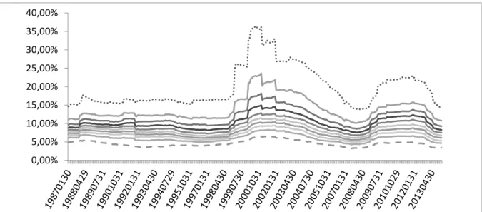
Figure 3: Realized ex-post total volatility across decile portfolios sorted by total volatility ... 76 Figure 4: Long term average of total volatility across decile portfolios ... 78

Introduction

1.1. Motivation and research questions

THE RELATION BETWEEN VOLATILITY AND EXPECTED STOCK RETURNS, BOTH TOTAL AND IDIOSYNCRATIC, IS CURRENTLY UNDER DEBATE. Investigating the relation between daily stock returns and 1-month lagged idiosyncratic volatility, Ang, Hodrick, Xing, and Zhang (2006) find that stocks with high idiosyncratic volatility relative to the Fama French three (FF-3) factor model have abysmally low average returns. The quintile with the lowest idiosyncratic volatility stocks outperforms the quintile with the highest idiosyncratic volatility stocks by 1.06% (t-statistic -3.10) in monthly average return. Their data sample is consisted of all stocks listed in AMEX, NASDAQ, and the NYSE from January 1986 to December 2000. Recently, the topic has been rekindled by Blitz and van Vliet (2007), Baker, Bradley, and Wurgler (2011), and Frazzini and Pedersen (2014). Blitz and van Vliet (2007) have a comprehensive analysis of the performance persistence of low total volatility stocks from 1985 to 2006 for all constituents of FTSE World Developed Index. Frazzini et al. (2014) find that betting-against-beta factor, which is longing low beta assets and shorting high-beta assets, produces significant positive risk-adjusted return. The limits of arbitrage and bias preference for high volatility and beta assets have been the main explanations for the anomaly. Baker et al. (2011) highlight a two-fold increase in institutional holding from 1968 to 2008. The authors attribute the lack of arbitrage activities to the hesitance of institutional investors, who are under tracking error and leverage constraints, to invest in high volatility stocks. The negative relation between volatility and expected returns as a stark contrast to the prediction of the traditional asset pricing has therefore attracted significant attention in academia.

Just as interesting as the effect that is believed to be the biggest anomaly in the financial history by Baker et al. (2011) is the emerging empirical evidence of the positive relation between various risk measures and expected stock returns. Using CRSP data from 1980 to 2004, Basu and Martellini (2007) find that the quintile with the highest total volatility stocks outperforms the quintile with the lowest total volatility stocks by 0.74% (p-value 1.37%) in monthly average return. As a response, Blitz and van Vliet (2011) challenge the result of Basu and Martellini (2007) on ground of using survivor stocks in the sample. Therefore, overcoming this survivorship bias would be a solid contribution to prior research. Fu (2009) challenges the robustness of the short estimation window used by Ang et al. (2006) by arguing that idiosyncratic volatility is time varying and therefore the lagged one month idiosyncratic volatility is not a good proxy for the current month expected risk. In the robustness section,

Ang et al. (2006), indeed, note that the increase in the length of the pre-defined beta estimation time window leads to the reduction in the outperformance of the bottom quintile portfolio with the lowest beta stocks against the top quintile portfolio with the highest beta stocks. The mentioned beta is the proxy for daily innovation in aggregate volatility, measured as the sensitivity of asset returns to daily changes in VIX. In response to Ang et al. (2006), Fu (2009) reports a positive relation between risk and expected return, using the EGARCH model to estimate idiosyncratic volatility rather than historical measure. Blitz and van Vliet (2011) also confirm that methodological choices can lead to less robust results for the low volatility anomaly. Most recently, Li, Sullivan, and García-Feijóo (2014) show that dropping penny stocks from their research data sample leads to the non-statistically significant return of the zero cost equally weighted portfolio that is formed by longing stocks with low FF-3 idiosyncratic volatility and shorting stocks with high FF-3 idiosyncratic volatility. Their data sample is consisted of CRSP stocks from 1963 to 2010. Without having dropping these lowly priced stocks, Li et al. (2014) would have reached the consistent conclusion with Ang et al. (2006) in favor of the low volatility effect. In a nutshell, the data sample and estimation window significantly drive differences in research results. 1

Overall, the empirical evidence of the low volatility effect serves the considerable academic interest in light of the ongoing debate between modern finance and behavioral finance. Eugene Fama and Robert Shiller, the respective key architect of the efficient market hypothesis (EMH) and behavioral finance, along with Lars Peter Hansen, were awarded the Nobel Prize in Economics in 2013. Under EMH, arbitrage opportunities will be quickly exploited to bring asset prices back to fundamentals. Behavioral finance proponents attribute to the limits of arbitrage as the reason for the considerably long persistence of anomalies, referring to the blind spot of EMH. The limits of arbitrage could arise due to different forms of frictions. Some of these common frictions come from (i) noise traders (see, e.g., De long, Shleifer, and Summers, 1990; Barber, Odean, and Zhu, 2009) (ii) limited capital (see, e.g., Shleifer and Vishny, 1997) (iii) short selling constraints (see, e.g., Mitchell, Pulvino, and Stafford, 2002; Barberis and Thaler, 2003) (iv) slow moving capital (v) arbitrageurs’ specialization (see, e.g., Shleifer and Vishny, 1997). In other words, even though prices could deviate from fundamentals, there is

1_{In the industry, unconstrained low volatility strategy is reported to deliver -1.1% in alpha per annum with respect}

to the Fama-French three factor model over the most updated data from 1986 to 2013 (Robecco, 2015). Low volatility asset ranks the worst among the researched asset classes in 2013 (State Street Advisors, 2013).

not necessarily abnormal return due to different constraints that discourage arbitrageurs from capitalizing on even known mispricing.

The purpose of this paper is to investigate whether the reported low volatility effect is present in an alternative data set that excludes penny stocks. I mainly focus on total volatility which has been studied to a lesser extent than idiosyncratic volatility or aggregate volatility (see, e.g., Campbell and Hentschel, 1992; Glosten, Jagannathan, and Runkle, 1993). I will focus on 12 month idiosyncratic volatility with respect to the FF-3 model only to the extent of testing the efficiency of the 3 portfolios. The choice of idiosyncratic volatility with respect to the FF-3 model rather than, e.g., CAPM, is due the wider application of the FF-FF-3 model in empirical finance. Importantly, the FF-3 model has been used by prior proponents of the low volatility effect (see, e.g., Blitz and van Vliet, 2007). Factor models generally advocate the existing systematic factors or any systematic factors orthogonal to those current ones should be priced. Many factor models, e.g., CAPM do not price idiosyncratic volatility as the variance of residuals can be eliminated by fair return risk trading. However, the empirical evidence for CAPM has been, if anything, weakened over the year (see, e.g., Gruber and Ross, 1978; Jobson and Forkie, 1982; Kandel and Stambaugh, 1987; Gibbons, Ross and Shanken, 1989; MacKinlay and Richardson, 1991). There has also been increasing evidence showing the explanatory power of the variance of the residuals in the cross section of expected returns (see, e.g., Lehmann, 1990; Goyal and Santa-Clara, 2003). Volatility and risk are not used interchangeably in my thesis, but not necessarily so in the literature review section. All the comparison, otherwise stated, refers to the comparison between the top volatility decile portfolio, decile 10 and the bottom volatility decile portfolio, decile 1. In this thesis, I answer the two main research questions as below.

Research question 1: Is there outperformance persistence of stocks with high total volatility and idiosyncratic volatility?

Following Fama and French (1992) to validate the value effect by sorting stocks based on firm size and book-to-market ratio into decile portfolios, I sort stocks into decile portfolios by volatility and control for the FF-3 factor exposure in decile portfolios. I also analyze decile portfolios’ industry components that could potentially characterize the portfolio performance. By forming equally weighted portfolios sorted by volatility on a monthly basis following prior research (see, e.g., Blitz and van Vliet, 2007), I inadvertently harvest equal weighting and possibly rebalancing premium that lead to the relatively high level of the monthly average

returns across the decile portfolios. The equal weighting scheme utilizes the size effect by giving more weight to small capitalization stocks in the absence of optimizing any objective function. DeMiguel, Garlappi, and Uppal (2009) report that the 1/N portfolios produce Sharpe ratios that are 50% higher on average than the mean–variance-optimized portfolios. On the other hand, portfolios weighted by market capitalization have been noted to underperform portfolios weighted by alternative weighting schemes, e.g., fundamental weighting (see, e.g., Arnott, Jason, and Philip Moore, 2005). Therefore, I also switch from the equal weighting to the market capitalization weighting to quantify the marginal weighting effect. An alternative rationality to understand the low volatility effect through weighting scheme is that market capitalization weighting is more likely to give more weight to low volatility stocks, which are more likely to be big companies. Ang et al. (2006) also report that the quintile portfolio with the highest idiosyncratic volatility stocks accounts for only a small proportion of the market value of the research data (only 1.9% on average). If market capitalization weighted portfolios underperform equally weighted portfolios, this evidence serves as an argument against the outperformance of low volatility stocks against high volatility stocks.

Research question 2: Is the portfolio with high total and idiosyncratic volatility stocks respectively riskier than the portfolio with low total and idiosyncratic volatility stocks by various measures?

A relevant question to ask is whether the portfolio with the highest volatility stocks is riskier than the portfolio with the lowest volatility stocks. If returns were to follow normal distribution, which is completely characterized by the first two orders of the distribution and the covariance matrix, volatility would be an adequate measure of risk. However, extreme ex-post events occur with a much higher probability than theoretically expected in the financial market, which has fat tail risk and whose return is well known to defy normal distribution. Fat tail risk is an ex-ante risk measure, calculated as the probability mass equal to an integral from minus infinity to a certain limit under a correct (often fat tail) distributional assumption. As a result, volatility based risk measure such as Sharpe ratio or the first two moments of the distribution may not capture all the risks in portfolios (see, e.g., Mandelbrot and Taylor, 1967; Fung and Hsieh, 1999; Francois and Bruno, 2001). Return distribution, especially skewness has also assumed the explanatory role for the preference for high volatility stocks which is more of a preference for skewness than for volatility itself (see, e.g., Baker et al., 2011; Kumar 2009; Barberis and Huang, 2008). For example, Barberis and Huang (2008) also model this preference for the

lottery-like stocks with the cumulative prospect theory of Tversky and Kahneman (1992) such that investors at equilibrium overweigh the tail and overprice stocks with positive skewness, leading to negative excess returns. Just as the notion of risk varies, so does the risk measure. For example, in order for the high volatility portfolio to be riskier than other portfolios, it is expected to underperform especially in meltdown market conditions when the marginal utility of wealth is high. Even though an asset is less risky ex-ante, an ex-post huge loss of low probability could already lead to capital redemption, creating the limit of arbitrage for investment funds which are under mandate to benchmark against, e.g., major indices. Therefore, understanding the higher order of the distribution of returns and investigating the performance of the high (low) volatility portfolio, especially in relation to benchmark and in the drawdowns as the ex-post realization of the ex-ante tail risk, will therefore also shed light on the riskiness of decile portfolios.

1.2. Contribution to existing literature

My research contributes to the emerging study with empirical evidence invalidating the controversial low volatility effect, for which there is a shortage of explanations in academia (see, e.g., Baker et al., 2011). To resolve this contemporary puzzling relation between expected stock returns and volatility, I overcome prior data bias, study the weighting scheme effect, quantify portfolio components, and measure the post-formation performance of the volatility sorted deciles with benchmark-based metrics.

The choice of the data sample has a critical role in the low volatility effect. Overcoming the survivorship bias in the research of Basu et al. (2007), I have the stock universe reconstituted annually and portfolio rebalanced monthly, with both the survivor and the non-survivor stocks that have at least two year historical data. Not using index components also removes the dependence on the discretionary stock choice method of index providers as well as the chance of overestimating returns by measuring only stocks that survive in the index. The overestimation due to studying only stocks that survive in the index can be as high as 2% (Graham, B., 1949). Prior research that reports the low volatility effect in international markets focuses mainly on the stock index constituents. For example, Blitz and van Vliet (2007) have their research on the FTSE World Developed index constituents and do not report the local risk-free rates in use. As discussed briefly in Section 1.1., Li et al. (2014) report that the low volatility effect becomes non-statistically significant after dropping penny stocks from the research data. Abnormal return from the low volatility effect are mainly concentrated among penny stocks,

which generally do not reflect available information as efficiently as the more actively traded ones and are more difficult to be traded in any meaningful volumes. In my data set, lowly priced stocks (less than $5) only constitute less than 0.21% of the dataset on annual average, in line with Li et al. (2014) as an independent research at the time of writing my thesis. As a robustness test, I replicate the research with the same data universe and method by Baker et al. (2011) and find results in line with the authors. However, changing the data universe and time period leads to the deviation in my research.

In terms of the historical time window and data frequency, I require that each stock has at least 24 month historical data available, following Baker et al. (2011). My goal is to estimate 48-month total volatility and 12-48-month idiosyncratic volatility. Blitz and van Vliet (2007) and Baker et al. (2011) estimate total volatility with 36-month and 60-month historical data respectively. As mentioned, Fu (2009) argues that lagged one month idiosyncratic volatility estimated with daily data used by Ang et al. (2006) is not a good proxy for the current month expected risk.

My methodological contribution centers on the weighting scheme and post-formation measurement. Prior published research focuses on either the value weighting scheme or the equal weighting scheme and therefore has not documented the weighting effect on volatility sorting strategy. Aiming to explain the effect from a novel angle of industry concentration, I also analyze the industry components of decile portfolios. The probability of the stocks of different industries falling into certain decile is studied through the constructed f value.

1.3. Limitations of the study

There could be a blend of various effects at the portfolio level leading to the bias of average returns estimation ostensibly attributed to volatility. On one hand, the forming and holding of portfolios might embed premium from the rebalancing on top of the equal weighting premium. As a result, the extra premiums lead to the relatively high level of the average returns of decile portfolios. On the other hand, the reconstitution drag could lead to a downward estimation of returns. By reconstituting the 1000 largest stocks by market capitalization every year, I essentially drop stocks that fail to keep up with the other stocks in terms of market capitalization. Specifically, the reconstitution is achieved by buying a stock at a high price when it reaches the 1000 largest cap threshold and selling the stock when it reduces in capitalization. The market capitalization change is very often due to the change in the share price. The

reconstitution process can require buying high and selling low, creating the drag on the performance of the decile portfolio. As above mentioned, the overestimation and underestimation, if any, is not necessarily homogenous among all deciles. Low volatility stocks are usually large cap companies with less risk of dropping out of the stock universe and therefore have less reconstitution drag. My research has not comprehensively separated these various effects.

Besides, my study is subject to the limitations of the FF-3 factor model. For example, (i) Fama et al. (1992) advocate that the size factor and value factor are systematic risk factors and the FF-3 factor model is a parsimonious asset pricing model. This risk-based prediction is that stocks more exposed to the HML factor should be riskier and are expected to earn higher returns. However, Daniel and Titman (1997) sort stocks firstly by firm size and book-to-market ratio and subsequently by the HML beta. The authors find that the stock portfolio with the higher value beta is neither riskier nor has higher returns. Lakonishok et al. (1994) find little support that value stocks underperform glamor stocks in such states as low GDP growth or low market returns of the world. To be fundamentally riskier, value stocks are otherwise expected to underperform in such states when the marginal utility of wealth is high. (ii) There are also potential (non-linear) hidden risk factors other than FF-3 factors. Regardless of these setbacks, FF-3 model still exposes partial excess returns explained by factor and size factor exposure in my study. Another minor setback is that my thesis does not take the full account of the time-varying nature of beta and volatility in the industry component analysis by subsampling the data period. Instead, the occurrence probability of industries in decile portfolios is calculated across the whole time series.2

1.4. Main findings

For portfolios sorted by total volatility, I find that the equally weighted top volatility decile portfolio statistically outperforms the equally weighted bottom volatility decile portfolio by

2_{For example, stocks of information technology and telecommunication service sector had relatively high beta in}

the global developed market during the peak of the dotcom bubble in 2000. However, as of January 2014, these sectors have among the lowest beta. The beta of the materials sector, however, was nearly twice its level in 2000 (State Street Global Advisor, 2014).

1.01% (t-statistic 2.94) in monthly average return. Monthly average returns increase monotonically with volatility and market beta in the decile portfolios. It is worth noting that the relatively high level of average returns is driven by the equal weighting premium and is not attainable with the market capitalization weighting scheme. Rebalancing premium could also have the compounding effect for portfolios in my research. The FF-3 alphas are stably flat rather than monotonically increase with volatility. Alpha varies by only 10bps between the first nine decile portfolios and significantly picks up for the highest volatility decile portfolio at 1.4% (t-statistic 4.35). Factor exposure explains excess returns the least in the most volatile portfolio. It is worth noticing that coefficients of determination, or R-squared, from the regressions of decile excess returns on FF-3 factor returns are the highest for the mid-range decile portfolios and decrease monotonically to the extreme high and low volatility deciles.

Component analysis shows that high (low) volatility decile is dominated by specific industries, while mid-range volatility deciles have the most equally distributed industry components. Decile 10 is most dominated by stocks of firms in “Services-Computer Programming, Data Processing, Etc.”, “Semiconductors & Related Devices” and “Services-Prepackaged Software” industry, which all make up 16.09% of decile 10 components. Decile 1 is also highly concentrated towards stocks of firms in “Electric Services” and “Electric & Other Services Combined” industry with the combined occurrence rate of 36.48%. Decile 9 also has a similar, yet less concentrated, industry component profile to that of decile 10. As a benchmark, stocks of the industry with the highest f value across decile 2 to decile 8, makes up only about 4.43% of decile components on average. One possible explanation in relation to the R-squared is that mid-range deciles, compared with the bottom and top total volatility sorted deciles, are more diversified industry wise and therefore returns of mid-range deciles are better explained by systematic factor exposure. The peculiarity nature of the computer and semi-conductor related industry that dominates decile 10 could well assume the explanatory role for the portfolio’s relatively high alpha.

The high volatility decile portfolio is more likely to underperform the market factor during meltdown periods and has more uncertainty below the benchmark threshold. Decile 10 has the biggest maximum drawdown -82.57% during the dotcom bubble and underperforms the FF-3 market factor portfolio in 13 out of the 20 months in which the factor portfolio has the lowest returns. Even one-time loss can already lead to a liquidity squeeze or a huge fund outflow that creates the limit of arbitrage. However, the portfolio of the most volatile stocks is more likely

to outperform the market factor in upmarket condition. In terms of return distribution, central moment analysis and Jacque-Bera test statistic show that returns of all decile portfolios defy normal distribution. The first two orders of lower partial moment also show that top decile portfolio has higher expected shortfall below hypothetical target return and sensibly more downside variance. Decile 10 has higher excess kurtosis, indicating tail risk but also more positive skewness below the target return than decile 1. Interestingly, I also find that the low volatility portfolio has a higher Sharpe ratio in line with the proponents of the low volatility anomaly. However, the higher Sharpe ratio of the low volatility decile is partially attributable to the extraordinarily small denominator. Choosing the right benchmark e.g., the expected shortfall below VAR, is outside the scope of the thesis and is the fund specific question that eludes a definite answer.

Switching from the equal weighting scheme to the market capitalization weighting scheme shows extremely interesting results. The market capitalization weighted decile portfolios yield abysmally small average returns and have an average alpha of -0.02% per month at 99% confidence level. The market capitalization weighted decile portfolios underperform the equally weighted counterpart portfolios and the market factor portfolio. There is no monotonic increase in FF-3 alpha nor beta from decile 1 to decile 10 as previously found in the equally weighted decile portfolios. All else equal, the abysmal monthly average returns and the underperformance of market capitalization weighted decile portfolios against the equally weighted counterparts can be explained by the overweight of large market capitalization stocks which on average have lower returns than small market capitalization stocks.

For portfolios sorted by idiosyncratic volatility, I also find a positive relation between average returns and idiosyncratic volatility in line with Fu (2009). The most noteworthy difference in average return 0.81% (t-statistic 2.79) is between decile 10 and decile 1. In addition, portfolios sorted by idiosyncratic volatility bear striking similarity to portfolios sorted by total volatility by various measures, including drawdown and return distribution below the benchmark target return.

1.5. Future research

Given the findings of this paper, it would be highly interesting to study a cost-based trading strategy of longing the 10% most volatile stocks in the presence of the equal weighting, the monthly rebalancing, and the annual reconstitution of the largest 1000 stocks by average yearly

market capitalization with a CRSP data sample. Furthermore, it is noted from my current research that volatility increases monotonically with average return but not with alpha. One hypothesis based on the component analysis is that the relatively high alpha of decile 10 might well be characterized by the dominating stocks of the computer programing and semiconductor device related industries. Dropping stocks of firms in these industries completely from the data set is an area for future research.

1.6. Structure of the study

The structure of this paper is as follows. Section 2 gives an overview of the literature on the relation between various proxies of risk and expected returns. In this section, I also review the weighting schemes and benchmark-based risk measurement that are relevant to my research. Section 3 presents the hypothesis. Section 4 clarifies the data and methodology on pre-formation parameter estimation and post-pre-formation portfolio measurement. Section 5 shows the results on the performance of portfolios sorted by volatility. Section 6 explains the robustness tests. Section 7 goes through the discussion on volatility sorting strategy in the current market environment as of the first quarter of 2015. Section 8 highlights the investment implication of the key main findings which answer the research questions.

Literature review

2.1. Empirical evidence for the relation between risk and expected returns

This section covers literature of the theoretical risk and return tradeoff as well as the controversial empirical evidence on the negative relation between average returns and various proxies for risk, including total volatility, idiosyncratic volatility, and beta.

2.1.1. On the non-positive relation between risk and expected returns

The evidence of risk return tradeoff in line with the Capital Asset Pricing model has been reported to be weaker over the years. Starting in the 1970s, Black, Jensen, and Scholes (1972) note that relation between risk and return was much flatter than that predicted by the CAPM. Haugen and Heins (1975) find that the relation is inverted. Later on, Reinganum (1981), Lakonishok, and Shapiro (1986) report that the positive relation between beta and average returns disappears when beta is used to explain average returns. In the same school of literature, Longstaff (1989) also find the cross sectional regression coefficient on the total variance for

size-sorted portfolios carries the insignificantly negative sign using CRSP monthly stock returns from 1926 to 1985. Fama and French (1992) astoundingly state that betas are “dead”. As discussed, Ang et al. (2006) find that the quintile portfolio with the lowest idiosyncratic volatility stocks outperforms the quintile portfolio with the highest idiosyncratic volatility stocks by 1.06% per month on average returns with listed equity on AMEX, NASDAQ, and NYSE from January 1986 to December 2000. Ang at al., (2006) advocate aggregate stochastic volatility as a negative priced risk factor that is orthogonal to other factors in the cross section of stock returns. The market price of aggregate volatility is reported at -1% per annum. Ang et al. (2006) argue that under such condition, investors demand the stocks that can hedge against market volatility. These stocks usually have higher loadings or sensitivities to market volatility factors. Investors have higher demand for stocks with higher exposure to market volatility, increasing its price and thereby reducing returns. Although Ang et al. (2006) do find that the quintile with the lowest idiosyncratic volatility stocks has higher average returns than the quintile with the highest idiosyncratic volatility stocks, they fail to explain that outperformance by using their model and related arguments. Such model prediction is that higher idiosyncratic volatility stocks would have higher exposure to the market volatility risk factor and therefore would be more desirable as the hedge assets. As a result, they have higher prices or lower expected returns.

Recently, the low volatility effect has been revived with recent discussions by Blitz and van Vliet (2007), Frazzini and Pedersen (2010), and Baker, Bradley, and Wurgler (2011). Blitz and van Vliet (2007) find the performance persistence of low volatility stocks in the data from 1985 to 2006 for all the constituents of FTSE World Developed index. Frazzini and Pedersen (2010) find that going long low beta assets and going short high beta assets produces a significant risk adjusted return in 20 international equity markets, treasury bonds, corporate bonds, and futures. For the equity market, they create the self-financing portfolio to proxy for “betting against beta” factor that is found to produce significant positive risk-adjusted returns. Looking at risk from another measure, Bali, Cakici, and Whitelaw (2009) study a measure of lottery-like return distribution and find a negative relation between the risk measure and returns.

Behavioral finance explanations for the non-positive relation between risk and expected returns Karceski (2002) explains high beta stocks are more likely to do better in the boom market and therefore are preferred. Recently, Baker et al. (2011) refer to the (i) irrational demand due to

high preference for lotteries, representativeness, and overconfidence. As a result, risk loving and irrational investors overpay for high risks (ii) benchmarking by money managers leading to the hesitance to deviate from benchmarks in the short run at the expense of long term returns. Interestingly, Baker et al. (2011) observe an increase in institutional holding from 30% to 60% when the volatility anomaly is reported in the US market from 1968 to 2008. They arguably explain the anomaly not being arbitraged because institutional investors, who have leverage constraints, are refrained from increasing tracking error by investing in low risk stocks. Black (1972) also associates the leverage constraint to the flat beta and return relation.

Other explanations relate the preference for high volatility stocks more to the preference for skewness than to volatility itself. Such preference is attributed to the preference for lotteries such that buying high volatility stocks that have positive skewness enables investors to benefit from small chance of winning in the short run regardless of even larger chance of loss. Different from Baker (2011), Kumar (2009) find that individual investors have preference for the lottery like pay-off stocks which are lowly priced, have high idiosyncratic skewness, and have high idiosyncratic volatility. Barberis and Huang (2008) also model this preference for the lottery like stocks with the cumulative prospect theory of Tversky and Kahneman (1992) such that agents overweigh the tail of the distribution. More importantly, they argue that the tail distribution can be priced. At equilibrium, cumulative prospect investors who overweigh the tail highly value positive skewness. As a result, high volatility stocks with high positive skewness can be overpriced and can even earn negative excess returns.

2.1.2. On the positive relation between risk and expected returns

Traditional financial theories take a long standing stance on the risk return tradeoff. Notably, the modern portfolio theory (MPT) by Markowitz (1952) states that the higher weight in risky assets is expected to have the higher compensation. The risk adverse investor maximizes the utility by choosing the suitable optimum in relation to the risk preference. In such an efficient market, investors realize above average returns only by taking above average risk that has ex-ante positive price. Capital Asset Pricing Model, by Treynor (1961), Sharpe (1964), Lintner (1965), Mossin (1966), and Black (1972), is derived from MPT in the condition that the market portfolio is mean variance efficient. Higher beta indicates higher risk in the mean variance framework since beta is the only factor that contributes to the risk of the portfolio that contains it.

The multifactor model of Merton (1973) and Ross (1976) proposes that risk premiums are dependent on the conditional covariance between asset returns and innovations in state variables. The Intertemportal Capital Asset Pricing (I-CAPM) model corrects the static assumption of one-period utility maximization in the standard Capital Asset Pricing model. In the I-CAPM model, investors price (i) the systematic market risk (ii) the risk of the unfavorable shift in investment opportunities. The second component overcomes the CAPM in a way that investment opportunity choices are time varying. Investors are assumed to be able to identify state variables that capture these uncertainties and construct portfolios that hedge against changes in these variables. In other words, investors are concerned about risks from both market returns and changes in the forecasts of future market returns. As a result, I-CAPM is a multi-factor model that has been tested with many variables such as the changes in interest rates, gold prices, and political stability. I-CAPM advocates a positive relation between risk and return for the aggregate stock market. The Arbitrage Pricing Theory by Ross (1976) is another multi-factor model that puts no particular significance on any multi-factor portfolio. The model is based on a linear return generating process, requiring no utility assumption beyond monotonicity and concavity or being restricted to a single period.

In general, factor models generally advocate that systematic risk factors e.g., systematic volatility should be priced in the cross section of returns. However, there is an increasing literature noting the explanatory power of idiosyncratic volatility in the cross section of expected returns. Lintner (1965) also show that idiosyncratic volatility, or the variance of residuals from the market model, significantly explains the cross section of average stock returns. However, Fama and Macbetch (1972) find the statistical pitfalls in the model of Lintner (1965). In the 90s, Lehmann (1990) report statistically significant positive coefficients on idiosyncratic volatilities in cross sectional regressions, reconfirming the above-mentioned finding of Lintner (1965). Lehman research data is monthly total returns for all the common stocks traded on NYSE as well as the equally weighted and the value weighted indices of their returns from 1926 to 1984. Idiosyncratic volatility has been found to be important in other markets. Green and Rydqvist (1997) find the idiosyncratic volatility premium on the Swedish lottery bond market. Malkiel and Xu (2002) report the portfolio with the highest idiosyncratic volatility stocks has the highest average return but did not report any significance levels for idiosyncratic volatility premium. Malkiel and Xu (2002) employ the models of Fama and Macbeth (1973) and Fama and French (1992) with the data on stocks on NYSE, AMEX, NASDAQ, and TSE from 1975 to 2000.

Goyal and Santa-Clara (2003) state that “idiosyncratic risk matters”. Focusing on the time series relation rather cross sectional and measuring idiosyncratic risk through the average of stock variance, they point out that market variance has no predictive power. The idiosyncratic volatility or the average variance of stock returns has a positive relation with the stock returns with CRSP data from 1962 to 1999. The relation is significant after the control of the macroeconomic variables that are the forecast of the stock market and can be explained from the traditional risk return compensation approach as well as the option approach. Looking at equity and debt as respective call option and put option, the value of equity goes up at the expense of debt holders as the volatility of the underlying assets increases. The correlation between average stock variance and the spread of A-rated bonds over treasuries is found to be at 0.7 from 1965 to 1999, consistent with negative impacts on bond returns but positive impacts on stock returns.

Fu (2009) use EGARCH model to estimate idiosyncratic volatility in cross sectional regressions to find its positive statistical significance as a rebuttal against Ang et al. (2006). Fu has a shark criticism of the one month lagged data window for estimating idiosyncratic volatility by Ang et al. (2006). Indeed, Ang et al. (2006) report that the longer the estimation period for pre-defined beta, the less the outperformance of the bottom beta portfolio. The quintile portfolio with the highest idiosyncratic volatility stocks lags behind the quintile portfolio with the lowest idiosyncratic volatility stocks by 0.53% (t-statistic -2.88), 0.37% (t-statistic -1.62) and 0.24% (t-statistic -1.04) with respective twelve month, three month and one month estimation period, in terms of FF-3 alpha.

The heated debate comes alive with emerging empirical evidence against the low volatility effect. As mentioned in the motivation, Basu and Martellini (2007) find that the quintile portfolio with the highest total volatility stocks outperforms the quintile portfolio with the lowest total volatility stocks by 0.74% (p-value 1.37%) with CRSP data from 1990 to 2004. As a response, Blitz and van Vliet (2011) challenge the result of Basu et al. (2007) on ground of using survivor stocks in the sample. Li et al. (2014) report that anomalous return is not found in the equally weighted portfolio betting on low idiosyncratic volatility with respect to the CAPM model. By dropping lowly priced stocks, the anomalous return disappears in a value weighted low minus high volatility portfolio. The data sample is CRSP monthly stock returns from 1963 to 2010.

2.2. Left tail risk and benchmark-based risk measures

This section presents literature on return distribution in the financial market and various benchmark-based risk measures.

2.2.1. Left tail risk

Mandelbrot (1963a, b) and Mandelbrot and Taylor (1967) are the very first to show that returns on financial markets are not normally distributed, but exhibit excess kurtosis. Most investment returns exhibit negative skewness and excess kurtosis, indicating left tail risk that can be overlooked by merely looking at volatility based measures such as Sharpe ratio. Often, fat tail risk refers to events beyond three standard deviations that happen with a probability much higher than predicted by the normal distribution due to the many asymmetries in the markets, returns, information, and investor behaviors (Focardi et al., 2003). Even two investments that have the equal mean and standard deviation and therefore the same Sharpe ratios can differ significantly in skewness and kurtosis, or tail risk (see, e.g., Keating and Shadwick 2002). Fung and Hsieh (1999) argue that the mean variance framework is simplistically suitable only for a quadratic utility function or for normally distributed returns, thus ignoring large negative returns or fat tails. With the same logic, volatility or VAR under normal distribution does not capture the fat tail risk as it neither adequately captures all the observations of empirical distribution nor informs the maximum loss. From a behavioral aspect, investors tend to have more aversion to the left tail events of the distribution than to the right hand ones, according to the Prospect Theory of Kahneman and Tversky (1979). Even when return distribution is symmetrical, volatility does not capture this distinction. Further studying distribution at smaller granularity, Longin and Solnik (2001) reject the null hypothesis of multivariate normality in positive tails and find that correlation of large negative returns does not converge to zero, but tend to increase with the threshold level.

2.2.2. Benchmark-based risk measure

Benchmarking has been one of the main explanations for the overpricing of high risk assets that dampens returns (see, e.g., Baker et al., 2011; Blitz and Vliet, 2007). Price, Price, and Nantell (1982), and Popova, Popov, Morton, and Yau (2006) introduce the higher order lower partial moments (LPMs), taking into account returns below the target threshold and the higher aversion to left tail events than to the right tail events in line with the Prospect Theory. LPM requires

fewer restrictive assumptions of utility function and probability distribution than the mean variance selection rule. LPM is defined as bellows:

𝐿𝑃𝑀ℎ(𝑅𝑝) = ∫ (𝑅 − 𝑟)_−∞ℎ 2𝑓𝑝(𝑅)𝑑𝑅 (1)

Where h is the target level and 𝑓𝑝(𝑅) represents the probability density function of returns of portfolio p (see Price et al., (1982).

𝐸([𝐿 − 𝑤𝑇_𝑅]+₎𝐾 ₍₂₎

Where w and R are the vectors of portfolio weights and return, L is the target return (or mean or zero), + denotes the positive values only, K is the degree of the order of the moments (K = 1, 2, 3, and 4), and E is an expectation operator. Keating et al. (2002) later develop the Omega function that integrates all the higher order moments into one single function by calculating directly from the observed distribution.

𝛺(𝐿) =∫ (1−𝐹_𝐿𝑏 (𝑟))𝑑𝑟

∫ 𝐹𝑎𝐿 (𝑟)𝑑𝑟

(3)

Where Ω is the Omega function, r is the one period return, L is the threshold return, (a, b) is the interval of return, and F(r) is the cumulative density function of returns. The numerator (denominator) is the probability weighted total gain (loss) with L as the threshold return. Ω is calculated as the integration of the respective function in the specified return interval. Assuming that the higher return and the less risk are the better options, the higher omega equates the better portfolio. Kazemi et al. (2003) present the mathematical derivation of this ratio of integration as the ratio of expected gain and loss, deriving the ratio of the call option price to the put option price as below: 𝛺(𝐿) =∫ (1−𝐹𝐿𝑏 (𝑟))𝑑𝑟 ∫ 𝐹_𝑎𝐿 (𝑟)𝑑𝑟 = ∫ (𝑚𝑎𝑥 (𝑥−𝐿,0)𝑓(𝑥)𝑑(𝑥)_𝐿𝑏 ∫ (𝑚𝑎𝑥 (𝐿−𝑥,0)𝑓(𝑥)𝑑(𝑥)_𝐿𝑏 = 𝐸(𝑚𝑎𝑥 (𝑥−𝐿,0) 𝐸(𝑚𝑎𝑥 (𝐿−𝑥,0)= 𝑒−𝑟𝑓∗𝐸(𝑚𝑎𝑥 (𝑥−𝐿,0) 𝑒−𝑟𝑓∗𝐸(𝑚𝑎𝑥 (𝐿−𝑥,0)= 𝐶(𝐿) 𝑃(𝐿) (4)

Later, Kaplan .P, (2004) generalizes that Omega falls under the spectrum of Kappa (𝐾_(𝑛)). 𝐾_(𝑛) is Omega when n=1, Sortino ratio when n=2 and other measures with higher n.

𝜇−𝐿 √𝐿𝑃𝑀𝑛(𝐿)

Where L is investor minimum acceptable “threshold” return and LPM is the higher order lower partial moment as above. It is proved that that Ω (L) = 𝐾₁(𝐿)+1. In this thesis, I mainly use the LPM formula introduced by Price et al., (1982) and Popova et al., (2006).

2.3. Portfolio weighting scheme

2.3.1. Market capitalization weighting

The capital asset pricing model advocates that market portfolio is mean variance optimal and therefore passive investors benefit the most by investing in the market portfolio, which has the highest Sharpe ratio. A common proxy for the market portfolio is the market capitalization weighted portfolio which merits broad equity market coverage, high trading liquidity, high investment capacity, and low maintenance cost (see, e.g., Armott et al., 2005). Capitalization weighting is a passive strategy that overweighs large capitalization companies that generally have strong fundamentals. However, market capitalization weighted portfolio has been rejected as a good proxy for the market portfolio. The underlying assumptions of MPT are very much in consensus to be too simplistic. Even if relaxing the requirement for a proxy, the disadvantage of market capitalization weighting is the overweight of overvalued stocks and underweight of undervalued stocks. Hsu (2006) shows that cap weighed portfolios suffer from return drag if prices are noisy relative to the movements of company fundamentals. In other words, the market capitalization weighting can have growth bias. Armott et al. (2005) state that market capitalization scheme is a particularly volatile way to measure companies’ size and its true value. They ultimately provide the mathematical derivations that cap weighted portfolios would on average produce negative alphas relative to its fair expected returns.

2.3.2. Alternative weighting

The pioneer in deviation from the market cap weighted indexation is Arnott et al. (2005) who find that the studied fundamental indexation index outperforms the market capitalization index by 1.97% per year from 1962 to 2004. They find that the market cap weighting tends to react strongly to the investor preference, e.g., the strong response to energy shift in the 1980s or technology stock in 1998-2001. On the other hand, the fundamental weighting indexing selects and weighs stable metrics of company size such as book value, revenue, and dividends. According to Arnott et al. (2005), the outperformance of fundamental indexation tends to be attributable to market mispricing, the exposure to distress factors, the superior market

construction, or the mixed of all those factors. However, they remain open to further study of the true value drivers for fundamental indexation.

One interesting issue raised by Arnott et al. (2005) is whether the fundamental indexation is value biased or growth bias. The outperformance of value stocks against growth stocks in both US and international markets has generally come under consensus among academics (see, e.g., Chan et al., 1991; Fama et al., 1992). However, a much less agreed upon issue is the explanation for it. For example, the value effect has been accounted for by both modern finance and behavioral finance. Fama and French (1996) explain returns from the value effect such that higher returns are compensated for higher risk. Therefore, the value effect is still consistent with EMH. Behavioral finance proponents argue that those abnormal returns are a result of mispricing from the market. Investors tend to extrapolate too far into the past and overpay for the growth stock (see, e.g., Lakonishok, 1994; Shiller, 2003). Fama and French (1996) rebut by saying that the mean reversion of earnings growth is shorter than the distressed premium period of at least five years. As a result, extrapolation based on growth is not the valid explanation. Besides, Fama and French (1996) argue that anomalies do not pass the economic significance test that the marginal benefit of exploiting information exceeds the marginal cost. As the controversy becomes heated and fierce, Shiller (2003) argues that if value stocks are riskier, value stocks should have performed worse than growth stocks in downtime periods. However, he finds the opposite evidence and that value stocks are not more volatile than growth stocks. Against this argument, Fama (1992) argues that return spread does not correlate with GNP and that variance is not the adequate proxy for portfolio risk. Hsu et al. (2006) argue that the fundamental indexation is not merely the value indexation although it is true that the fundamental index under weighs growth stocks and tilts towards stocks with low P/E ratios and high dividend yields. They show the empirical evidence that U.S. Fundamental index 1000 outperforms Russell 1000 value and that the fundamental index outperforms the S&P 500 both in up and down markets. Value indexes are based on market capitalization and under weigh many growth companies that are growing their fundamentals equally rapidly while fundamental indexes don’t under weigh growth companies that are growing in fundamentals.

Estrada J., (2006) and Perod A., (2007) also advocate the fundamental indexing over the market cap weighted by exploring different company specific metrics. The indexation proliferates in categories, including tiled factors such as size, value, and momentum factor. Among others, equal weighting scheme utilizes the size effect of giving more weight to small stocks in the

absence of optimizing any objective functions (see, e.g., Clarke, de Silva, and Thorley, 2006; DeMiguel, Garlappi, and Uppal, 2009). DeMiguel et al. (2007) find that of that 1/n rule, or naïve diversification, is better than all 14 sample-based mean variance model across seven empirical data sets in terms of Sharpe ratio, certainty-equivalent return, or turnover. The results show that optimal diversification benefit is more than offset by estimation error, suggesting a long way for “optimal” portfolio choice to be realized out of sample.

Hypothesis

H1: There is performance persistence of stocks with high total volatility and idiosyncratic volatility.

H1a: The portfolio with high total and idiosyncratic volatility stocks respectively outperforms the portfolio with low total and idiosyncratic volatility stocks in monthly average return. Traditional asset pricing which advocates volatility as a risk measure and a positive linear relation between risk and expected returns predicts that higher risk is compensated with higher returns. That the portfolio with low volatility stocks outperforms the portfolio with high volatility stocks therefore presents an anomaly under such framework.

H1b: The value effect and size effect cannot explain the average returns of the portfolios sorted by total volatility and idiosyncratic volatility.

In order to examine whether the low volatility effect is another representation of the value effect and size effect, I control for value and size factor exposure by the multivariate ordinary least square regression analysis with the FF-3 factor model as following:

𝐸_(𝑟𝑖) = 𝛼 + 𝛽_1𝑖(𝑅_𝑚− 𝑅_𝑓) + 𝛽_2𝑖𝑆𝑀𝐵 + 𝛽_3𝑖𝐻𝑀𝐿 (6)

Where 𝐸_(𝑟𝑖) is the expected return on stock i, SMB (Small minus Big) is the average return on the three small portfolios minus the average return on the three big portfolios, HML (High minus Low) is the average return on the two value portfolios minus the average return on the two growth portfolios, (R_m− R_f) is the excess return on the market, β_1i and β_2i are the factor loading coefficients, and α is the alpha return. If α is significantly different from zero, the returns from decile portfolios are not adequately explained by the size and value factor

exposure. If α is not significantly different from zero, the size and value factor exposure explain all the excess returns.

H1c: Equally weighted decile portfolios sorted by total volatility and idiosyncratic volatility respectively outperform market capitalization weighted counterpart portfolios.

In the mean variance framework, the market portfolio is the most efficient portfolio with the highest Sharpe ratio. A common proxy for the market portfolio is the passive market capitalization portfolio. However, if the market capitalization weighted portfolio does not represent the set of all investable options or mean variance efficiency does not hold, investing in the market capitalization weighted index may not offer the best risk and return tradeoff. As a result, there could be chances to exploit the inefficiency with an alternative weighting. The equal weighting scheme that gives more weight to small market capitalization stocks could benefit from the size effect. As a result, the equally weighted portfolios could outperform the market capitalization counterpart portfolios.

H2: The portfolio with high total and idiosyncratic volatility stocks is respectively riskier than the portfolio with low total and idiosyncratic volatility stocks by various measures.

Normally distributed returns are fully characterized by the mean vector and the covariance matrix. Therefore, volatility is an adequate risk measure in the mean variance framework. However, if return distribution is not normally distributed, more volatile portfolios are not necessarily riskier. Theoretically, risk has an ex-ante positive price with a predicted distribution. However, the empirical realization of the ex-post risk return payoff can be negative at times.

Data and methodology

4.1. Data

My research data set is consisted of the largest 1000 listed stocks across US for the period from January 1983 to December 2013. The data is retrieved from CRSP for all stocks that are listed on AMEX, NASDAQ, and NYSE. The data set is monthly total returns that include both capital gains and dividends. North American value, size, momentum factor and monthly Treasury bill as the short term interest are downloaded from the Kenneth French library. Standard Industrial Classification (SIC) codes are downloaded from the website of Securities and Exchange

Commission. The SIC in a company's disseminated EDGAR filings indicates the company's type of business.

I start with all stocks listed in the CRSP database and require that the stock have at least 24 data point of historical data. Even large capitalization firms e.g., Berkshire Hathaway don’t always have reported prices or have missing data points in the data base. Therefore, I allow for the flexibility if there is an acceptable number of missing data points by first sorting by number N of observations by PERMNO and constrain N to have at least 20 to 24 historical data points. The data set is balanced annually so that stocks whose market capitalization rise below the threshold of top 1000 stocks by the market cap will be dropped out and stocks whose market capitalization drop below the threshold are included. I calculate the market capitalization based on the “Price or Bid Ask Average” and “SharesOutstanding”. In order to smooth out the fluctuation of monthly market cap, I calculate the average monthly market cap every year. The average market capitalization of these firms has also increased from $1.57bn to $20.76bn and the firm with the largest monthly average cap is Apple in 2012 at $547bn. Outliner stock price is that of Berkshire Hathaway Inc. Del with share price of $145 875 in January, 2013. I rank stocks by average market capitalization throughout the year to keep the top 1000 PERMNO with the highest market cap and retrieve holding period returns in each year. For each list of stocks corresponding to each year, I separately retrieve a set of 60 month historical data. Lowly priced stocks account for an insignificant proportion in my dataset at 0.21% on average across the year.

4.2. Methodology

4.2.1. Pre-formation total volatility estimation and post-formation measurement

4.2.1.1. Pre-formation parameter estimation Trading strategy

As discussed, my goal is to use up to 48 months of historical information to form portfolios and to monitor the portfolio for the next 12 months on a rolling basis. The portfolio is formed based on the ranking of ex-post realized total volatility calculated based on 48 month historical data. I define it as the preformation period. Portfolio formation strategies are based on an estimation period of E months, an awaiting period of W months, and a holding period of H months. The E/W/H strategy is as follows. At month t, I compute total volatilities from historical monthly

data over an E month period from month t−E−W to month t −W. At time t, I construct equally weighted portfolios based on these total volatilities and hold these portfolios for N months. My main analysis is based on the 1/0/1 strategy, in which I simply sort stocks into decile portfolios based on their level of total volatility computed using monthly returns over the past 48 months. I hold these equally weighted portfolios for 1 month. For simplicity, this strategy is written as 48/0/1. The decile portfolios are rebalanced each month. I also examine the robustness of my results to various choices of E, W, and H. The construction of the E/W/H portfolios for E>1 and M>1 follows Jegadeesh and Titman (1993) and Ang (2006) except that my portfolios are equally weighted. I have three variations as 36/0/1, 48/0/3, and 48/0/12. I will present those variations of holding period and estimation period in Section 6.

Ranking

Every month, I calculate the volatility of stocks return over the past four year on the rolling basis. Monthly returns have more stable informational content than weekly returns as used by Blitz and van Vliet (2007). For each month, I rank the total volatility and construct the decile portfolio following Fama (1992) methodology such that stocks are allocated in an independent sort to ten volatility group based on the ranking. I divide the ordered data into ten essentially equal-sized data subsets of 100 stocks. Stocks with the lowest 100 ranking scores are assigned to the bottom decile, decile 1 while stocks with the highest 100 scores are assigned to the top decile, decile 10. Scores are compared directly across all stocks without imposing sector or country restrictions.

Weighting scheme

For equal weighting scheme, I construct the equally weighted portfolio for each decile obtained by ranking stocks on the past four-year volatility of monthly returns on a rolling basis at the end of each month. Each stock is given weight 1/N (7) (N=100). The portfolio is form and hold from month t to t+1. For market cap weighting scheme, the cap weighted portfolio returns are calculated each month by multiplying stock returns with its corresponding weight in the decile portfolio. The market cap weight of stock i at month t is calculated by dividing its month end market cap by the month end sum of the market cap of all the stocks in the decile. The weighting calculation follows the formula 𝑤_𝑡 = 𝑀𝐶𝑖𝑡

∑ 𝑀𝐶𝑛1 𝑖𝑡

at month t, 𝑀𝐶_𝑖𝑡 is the month end market cap of stock i at month t, and n is the number of all stocks in each decile.

4.2.1.2. Post-formation measurement

Test period portfolios are monitored in several different ways. I run the regressions of the excess returns of test period portfolios on FF-3 factor returns to estimate alpha and factor loadings. The performance of test period portfolios are measured in terms of key statistics, return distribution, and benchmark-based measure. Average return and standard deviation are measured in monthly percentage terms and apply to total, not excess, simple returns. In order to separate the low volatility effect from other effects, I use the multivariate regression method with the FF-3 market factor, the SMB (small-minus-big), and the HML (high-minus-low). By regressing the excess returns of the volatility sorted portfolios on these factor returns, I investigate how much of decile excess returns is attributed to the value and size effect. An alternative way is to use the double sorting strategy. Firstly, I can sort stocks by the size and value factor that are desirable to be controlled into deciles. Subsequently, I can sort stocks into decile portfolios by total volatility within each decile.

Component analysis

I construct the f value by counting the occurrence frequency that an industry appears in each decile across the whole time series. In the initial step, I create a list of components for each decile in certain year. As the stocks are rebalanced, the stocks can drop in and out of the decile every month by switching between different deciles. Random falls in deciles are immaterial. I trace back the industry to which each of the stock PERMNO belongs according to Standard Industrial Classification (SIC). After converting the PERMNO data into SIC data, I calculate the frequency f that certain industry appears in certain decile. F is calculated as the number of time an industry appears in a decile divided by the total number of time all industries appear in that decile.

𝑓_𝑖𝑗 =𝑛𝑖𝑗

𝑁𝑗 (9)

where n=1 if industry i appears in decile j otherwise 0 and N is total number of time all industries appear in decile j.