Automatic Steering Methods for Autonomous Automobile Path Tracking

(1)

Automatic Steering Methods for Autonomous

Automobile Path Tracking

Jarrod M. Snider

CMU-RI-TR-09-08

February 2009

Robotics Institute

Carnegie Mellon University

Pittsburgh, Pennsylvania

c

(2)

Abstract

This research derives, implements, tunes and compares selected path tracking methods for controlling a car-like robot along a predetermined path. The scope includes commonly used methods found in practice as well as some theoretical methods found in various literature from other areas of research. This work reviews literature and identifies important path tracking models and control algorithms from the vast background and resources. This paper augments the literature with a comprehensive collection of important path tracking ideas, a guide to their implementations and, most importantly, an independent and realistic comparison of the performance of these various approaches. This document does not catalog all of the work in vehicle modeling and control; only a selection that is perceived to be important ideas when considering practical system identification, ease of implementation/tuning and computational efficiency. There are several other methods that meet this criteria, however they are deemed similar to one or more of the approaches presented and are not included. The performance results, analysis and comparison of tracking methods ultimately reveal that none of the approaches work well in all applications and that they have some complementary characteristics. These complementary characteristics lead to an idea that a combination of methods may be useful for more general applications. Additionally, applications for which the methods in this paper do not provide adequate solutions are identified.

(3)

Acknowledgements

This work would not have been possible without the support, motivation and encouragement of Dr. Chris Urmson, under whose supervision I chose this area of research. I would like to acknowledge the advice and guidance of Dr. William ”Red” Whittaker, whom never ceases to amaze and inspire me. Special thanks go to Tugrul Galatali, whose knowledge and assistance was instrumental in the success of this research and paper.

I acknowledge Mechanical Simulation for their generous support and discount of CarSim. Without CarSim, quality analysis and comparison of tracking methods may not have been possible.

I would also like to thank the members of my family, especially my wife, Amy, and my son Xavier for supporting and encouraging me in everything I do.

(4)

List of Figures

1 Sandstorm . . . 1

2 Stanley . . . 1

3 Boss . . . 1

4 Screen shot from a CarSim animation . . . 3

5 Lane Change Course . . . 4

6 Figure Eight Course . . . 5

7 Road Course . . . 6

8 Velocity profiles used on the Road Course . . . . 7

9 Geometric Bicycle Model . . . 8

10 Pure Pursuit geometry . . . 9

11 Pure Pursuit at multiple speeds and various gains on the lane change course . . . 11

12 Pure Pursuit at multiple speeds and various gains on the figure eight course . . . 12

13 Pure Pursuit at multiple velocity profiles and various gains on the road course . . . 13

14 Stanley method geometry . . . 14

15 Stanley controller at multiple speeds and various gains on the lane change course . . . 15

16 Stanley controller at multiple speeds and various gains on the figure eight course . . . 16

17 Stanley controller at multiple velocity profiles and various gains on the road course . . . 17

18 Kinematic bicycle model . . . 18

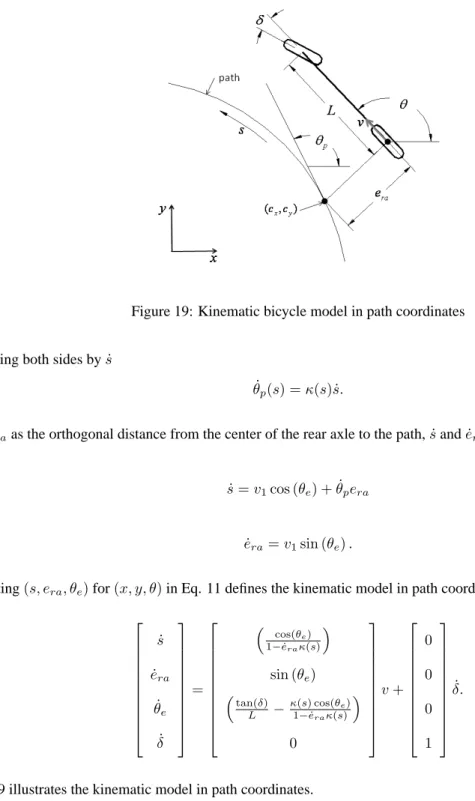
19 Kinematic bicycle model in path coordinates . . . 21

20 Kinematic controller at multiple speeds and various gains on the lane change course . . . 26

21 Kinematic controller at multiple speeds and various gains on the figure eight course . . . 27

22 Kinematic controller at multiple velocity profiles and various gains on the road course . . . 28

23 Dynamic Bicycle Model . . . 29

24 Dynamic Bicycle Model in path coordinates . . . 31

25 Example of lateral force tire data . . . 34

26 Linear approximation of the lateral force tire data . . . 34

27 LQR controller at multiple speeds and various gains on the lane change course . . . 39

(7)

30 LQR controller with feed forward term at multiple speeds and various gains on the lane change course 44 31 LQR controller with feed forward term at multiple speeds and various gains on the figure eight course 45 32 LQR controller with feed forward term at multiple velocity profiles and various gains on the road course 46 33 Optimal preview controller with 0.5s preview at multiple speeds and various gains on the lane change

course . . . 49

34 Optimal preview controller with 1.0s preview at multiple speeds and various gains on the lane change course . . . 50

37 Optimal preview controller with 0.5s preview at multiple speeds and various gains on the figure eight course . . . 53

41 Optimal preview controller with 0.5s preview at multiple speeds and various gains on the road course 57 42 Optimal preview controller with 1.0s preview at multiple speeds and various gains on the road course 58 43 Optimal preview controller with 1.5s preview at multiple speeds and various gains on the road course 59 44 Optimal preview controller with 2.0s preview at multiple speeds and various gains on the road course 60 45 Comparison of the tuned controllers on the lane change course . . . 61

46 Comparison of the tuned controllers on the figure eight course . . . 62

47 Comparison of the tuned controllers on the road course . . . 63

(8)

1 Introduction

A significant portion of Robotics research involves developing autonomous car-like robots. This research is often at the forefront of innovation and technology in many areas. However, it is often common practice to use relatively simple and sometimes naive control strategies and/or system models for vehicle control, even on some well known and successful autonomous vehicle projects [18, 17, 16, 4].

Figure 1: Sandstorm

Figure 2: Stanley

Figure 3: Boss

Figure 1 is Sandstorm, the autonomous vehicle that placed second in the DARPA Grand Challenge using a very simple steering control law based on a geometric vehicle model. Figure 2 is Stanley, the autonomous vehicle that won the DARPA Grand Challenge using an intuitive steering control law based on a simple kinematic vehicle model. Figure 3 is Boss, the autonomous vehicle that won the DARPA Urban Challenge. Boss uses a much more sophisticated

(9)

not mean, however, there has not been extensive research in this area, and a great deal of literature on the topic exists. These observations lead to the following questions:

• How good are these simple methods commonly found in practice?

• Can improvements in performance be achieved using existing methods found in other theoretical research? • Can good matches between methods and applications be identified?

• What are the limitations and potential for future breakthroughs?

It is these observations and questions that motivate the research found in this paper. This paper endeavors to collect scattered sources and provide an independent and realistic comparison of the performance of several classes of vehicle controllers along with advice on how to implement them.

The family of vehicle controllers of interest are called path trackers. Path tracking refers to a vehicle executing a globally defined geometric path by applying appropriate steering motions that guide the vehicle along the path. The goal of a path tracking controller is to minimize the lateral distance between the vehicle and the defined path, minimize the difference in the vehicle’s heading and the defined path’s heading, and limit steering inputs to smooth motions while maintaining stability.

For each class of path trackers presented in this paper, an underlying system model will be developed before the algorithm is presented. The algorithms themselves will be presented in a way to minimize the complexity of performance tuning, and the effects of the parameters will be illustrated using three representative courses. Chapter 2 will concentrate on methods that exploit geometric relationships between the vehicle and the path to design control laws [2, 16] that are simple, robust and achieve accurate path tracking in a limited set of driving scenarios and can provide moderate tracking in a much larger set of scenarios. Chapter 3 moves on to more control theory based techniques and uses a simple kinematic model of a vehicle [6] to show that accurate path tracking can be achieved with this simple model in a limited set of driving scenarios. Chapter 4 introduces a dynamic vehicle model and techniques such as Optimal Control and Optimal Preview Control [11, 10, 14] to demonstrate that accurate path tracking can be achieved over a wider range of driving scenarios when the dynamics of the vehicle are considered. Chapter 5 then turns to a head-to-head performance comparison of these algorithms which illustrates why relatively primitive control techniques are commonly used successfully as well as highlighting the need for more advanced techniques as Robotics moves forward in the development of precision path tracking for vehicles operating at higher speeds and with new objectives.

(10)

1.1 Experimental Design

Figure 4: Screen shot from a CarSim animation

To provide a valid evaluation and comparison, the path tracking controllers implemented for this paper are tested with a high fidelity vehicle simulator, CarSim. CarSim quickly and accurately simulates the dynamic behavior of vehicles and is used in the automotive industry as the standard by which vehicle handling and dynamics are tested [1]. Figure 4 is a screen shot from a CarSim animation. The standard CarSim simulator provides a complete model of the vehicle system and the environment [7]. Additionally, rate limits and delays associated with the steering actuator are added to the standard model. The controllers are implemented in C and communicate with CarSim through the available API [8].

Three driving courses are chosen to perform the various experiments found in this paper. The courses are designed to test attributes of the controllers and provide insight into their relative advantages and disadvantages.

1.1.1 Lane Change Course

The Lane Change Course is a straight section of two lane road in which the vehicle is required to perform a single lane change maneuver. The lane change maneuver is a common test for vehicle handling as it represents an essential collision avoidance maneuver. The Lane Change Course is chosen to demonstrate the tracking capability on a straight path as well as the response to a quick, yet (position and curvature) continuous, transient section. Experiments on this course are performed at constant velocities of 5m/s, 10m/s, 15m/sand 20m/s. Figure 5 illustrates the Lane Change

(11)

Figure 5: Lane Change Course

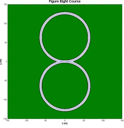
1.1.2 Figure Eight Course

The Figure Eight Course consists of two circular paths that intersect at a tangent point. This course is not com-monly found in everyday driving. However, it can provide valuable insight into the handling of a vehicle as well as some important characteristics of a controller. This course was chosen to illustrate the steady state characteristics of the controllers while executing a constant nonzero curvature path. This course also includes a point with discontinuous curvature where vehicles transition from one circle to an other. While it is possible to require that all paths be generated with continuous curvature, a controller’s response to this discontinuity provides insight into it’s robustness. Experi-ments on this course are performed at constant velocities of 5m/s, 10m/s, 15m/sand 20m/s. Figure 6 illustrates the Figure Eight Course.

(12)

Figure 6: Figure Eight Course

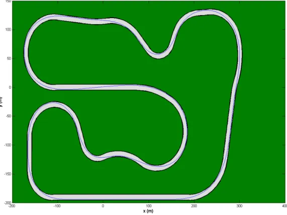
1.1.3 Road Course

The Road Course captures a variety of driving scenarios representative of real-world driving. The path is generated to minimize lateral acceleration while staying on the road surface. The path is continuous and the speed varies as a function of the path. The Road Course facilitates a general performance comparison of the various tracking methods. Figure 7 illustrates the Road Course.

(13)

(14)

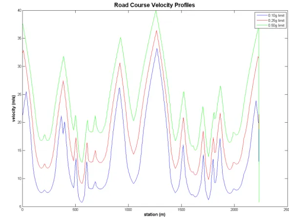
Experiments on this course are performed at three different velocity profiles. The velocity profiles are generated to limit the longitudinal acceleration to within a range a vehicle could achieve while also limiting the theoretical kinematic centripetal acceleration of the vehicle. The longitudinal acceleration is limited to be between -4m/s2_and 3m/s2 _{for all experiments. The three velocity profiles are generated with kinematic centripetal accelerations limits} of 0.1g, 0.25gand 0.5g. Despite these kinematic limitations, the actual lateral acceleration of the vehicle can be much greater in magnitude. The velocity profiles for this course are illustrated in Figure 8.

(15)

2 Geometric Path Tracking

One of the most popular classes of path tracking methods found in robotics is that of geometric path trackers. These methods exploit geometric relationships between the vehicle and the path resulting in control law solutions to the path tracking problem. These techniques often make use of a look ahead distance to measure error ahead of the vehicle and can extend from simple circular arc calculations to more complicated calculations involving screw theory [19]. This section will describe the geometric vehicle model most commonly used by these methods and two of these methods: Pure Pursuit and the Stanley Method.

2.1 Geometric Vehicle Model

Figure 9: Geometric Bicycle Model

A common simplification of an Ackerman steered vehicle used for geometric path tracking is the bicycle model. Section 3.1 includes a detailed discussion of Ackerman steering and the kinematics of the bicycle model. For the purpose of geometric path tracking, it is only necessary to state that the bicycle model simplifies the four wheel car by combining the two front wheels together and the two rear wheels together to form a two wheeled model, like a bicycle. The second simplification is that the vehicle can only move on a plane. These simplifications result in a simple geometric relationship between the front wheel steering angle and the curvature that the rear axle will follow. As shown in Figure 9, this simple geometric relationship can be written as

tan(δ) = L

(16)

whereδis the steering angle of the front wheel,Lis the distance between the front axle and rear axle (wheelbase) and

Ris the radius of the circle that the rear axle will travel along at the given steering angle. This model approximates the motion of a car reasonably well at low speeds and moderate steering angles.

2.2 Pure Pursuit

Figure 10: Pure Pursuit geometry

The pure pursuit [2] method and variations of it are among the most common approaches to the path tracking problem for mobile robots. The pure pursuit method consists of geometrically calculating the curvature of a circular arc that connects the rear axle location to a goal point on the path ahead of the vehicle. The goal point is determined from a look-ahead distance ℓd from the current rear axle position to the desired path. The goal point(gx, gy)is

illustrated in Figure 10. The vehicle’s steering angleδcan be determined using only the goal point location and the angleαbetween the vehicle’s heading vector and the look-ahead vector. Applying the law of sines to Figure 10 results in ℓd sin (2α)= R sin π 2 −α ℓd 2 sin (α) cos (α)= R cos (α) ℓd sin (α) = 2R

(17)

or

κ=2 sin (α)

ℓd

, (2)

whereκis the curvature of the circular arc. Using the simple geometric bicycle model of an Ackerman steered vehicle from Section 2.1, the steering angle can be written as

δ= tan−1₍_κL₎_. ₍₃₎

Using Eq. 2 and 3, the pure pursuit control law is given as

δ(t) = tan−1 2Lsin(α(t)) ℓd .

A better understanding of this control law can be gained by defining a new variable,eℓdto be the lateral distance

between the heading vector and the goal point resulting in the equation

sin (α) =eℓd

ℓd

.

Eq. 2 can then be rewritten as

κ= 2

ℓ2

d

eℓd. (4)

Eq. 4 demonstrates that pure pursuit is a proportional controller of the steering angle operating on a cross track error some look-ahead distance in front of the vehicle and having a gain of2/ℓ2

d. In practice the gain (look-ahead distance)

is independently tuned to be stable at several constant speeds, resulting inℓdbeing assigned as a function of vehicle

speed.

2.2.1 Tuning the Pure Pursuit Controller

To simplify tuning, the control law can be rewritten, scaling the look-ahead distance with the longitudinal velocity of the vehicle. Scaling the look-ahead distance in this manner is a common practice. Addionally, the look-ahead distance is commonly saturated at a minimum and maximum value. In this paper these value are set to 3m and 25m respectively. This results in

δ(t) = tan−12Lsin(α)

kvx(t)

(18)

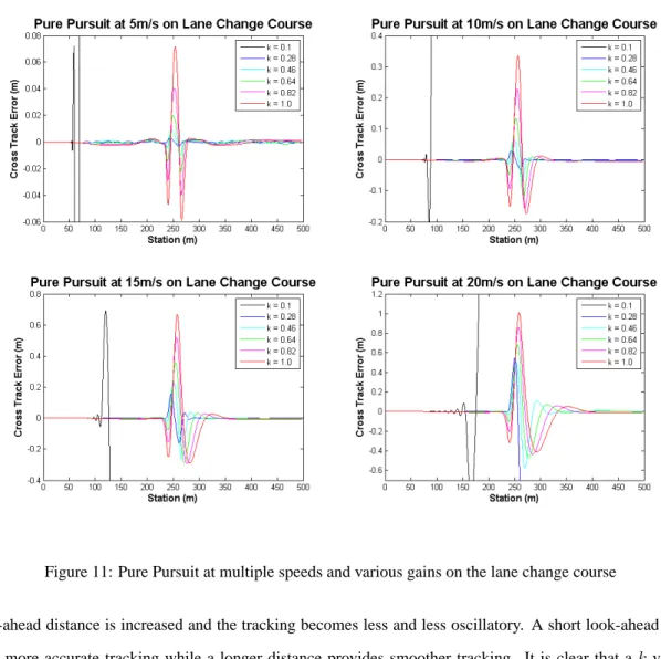
Experiments are conducted on the Lane Change Course. Figure 11 illustrates the effects of the tuning parameter on tracking performance during these experiments. The tracking results are what one might expect. Askincreases

Figure 11: Pure Pursuit at multiple speeds and various gains on the lane change course

the look-ahead distance is increased and the tracking becomes less and less oscillatory. A short look-ahead distance provides more accurate tracking while a longer distance provides smoother tracking. It is clear that ak value that is too small will cause instability and akvalue that is too large will cause poor tracking. Another characteristic of Pure Pursuit is that a sufficient look-ahead distance will result in ”cutting corners” while executing turns on the path. The trade off between stability and tracking performance is difficult to balance with Pure Pursuit and will begin to seem course dependent. This is in part due to the fact that the Pure Pursuit method ignores the curvature of the path. Intuition would leave one to believe that the curvature of the path should somehow influence the look-ahead distance as well as the velocity (and perhaps even the current local cross track error). The effects of this will be seen in further

(19)

of Pure Pursuit.

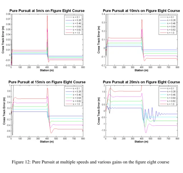
Experiments are conducted on the Figure Eight Course. Figure 12 illustrates the effects of the tuning parameter on tracking performance during these experiments. Again, similar results are obtained. The good characteristic to

Figure 12: Pure Pursuit at multiple speeds and various gains on the figure eight course

point out during this test is that the Pure Pursuit method is robust to the discontinuity in the path. It is clear to see that on a constant curvature path a value ofkcan always be chosen that will perform well on that curvature, but could fail miserably when presented with a different curvature or different speed. This is because Pure Pursuit is simply calculating a circular arc based on the simple geometric model of the vehicle. In this case there is clearly a circular arc the vehicle would have to travel to stay on the path, but the vehicle travels a different circular arc than what the model would predict. This discrepancy comes from the model ignoring the vehicle’s lateral dynamic characteristics that are more and more influential as the speed and/or curvature increases. It is easy to imagine that in constant curvature and constant speed tests this dynamic effect can be compensated for by increasingkuntil the circular arc that is computed is tighter than the circular arc of the path at a proportion that would cancel out the dynamic side slip of the vehicle.

(20)

This is a bad characteristic for tuning the tracker. One must be careful not to over tune on a course and test a variety of courses and speeds to find akthat can perform well over the operating space of the vehicle. This usually results in giving up accuracy to insure stability. Again, the final test is not typical of of most driving scenarios.

Experiments are conducted on the Road Course. Figure 13 illustrates the effects of the tuning parameter on tracking performance during these experiments. The ”cutting corners” is apparent again in this test. However, Pure Pursuit can

Figure 13: Pure Pursuit at multiple velocity profiles and various gains on the road course

be tuned to perform reasonably well on this course. The 0.5g test is simply an analysis tool and may not be a test that a tracker should be able to complete. It is valuable to know how and under what conditions a method will fail.

The characteristics of Pure Pursuit during tuning can be summarized as follows: Decreasing the look-ahead dis-tance results in higher precision tracking and eventually oscillation, and increasing the look-ahead disdis-tance results in lower precision tracking and eventually stability.

(21)

2.3 Stanley Method

Figure 14: Stanley method geometry

The Stanley method [16] is the path tracking approach used by Stanford University’s autonomous vehicle entry in the DARPA Grand Challenge, Stanley. The Stanley method is a nonlinear feedback function of the cross track error

ef a, measured from the center of the front axle to the nearest path point(cx, cy), for which exponential convergence

can be shown [16]. Co-locating the point of control with the steered front wheels allows for an intuitive control law, where the first term simply keeps the wheels aligned with the given path by setting the steering angleδequal to the heading error

θe=θ−θp,

whereθis the heading of the vehicle andθpis the heading of the path at(cx, cy). Whenef a is non-zero, the second

term adjustsδsuch that the intended trajectory intersects the path tangent from(cx, cy)atkv(t)units from the front

axle. Figure 14 illustrates the geometric relationship of the control parameters. The resulting steering control law is given as δ(t) =θe(t) + tan−1 _ke f a(t) vx(t) , (5)

wherekis a gain parameter. It is clear that the desired effect is achieved with this control law: Asef aincreases, the

(22)

2.3.1 Tuning the Stanley Controller

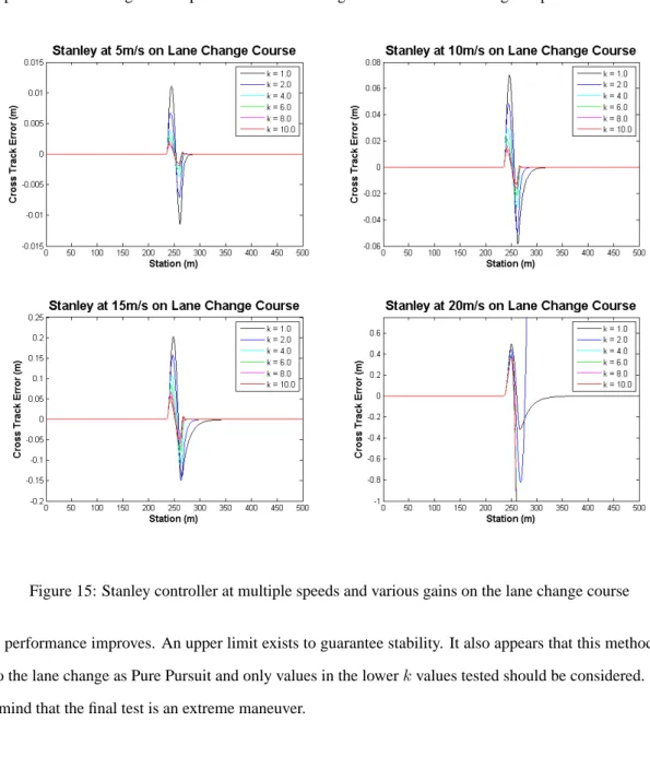
Experiments are conducted on the Lane Change Course. Figure 15 illustrates the effects of the tuning parameter on tracking performance during these experiments. The tracking results are what one might expect. Askis increased the

Figure 15: Stanley controller at multiple speeds and various gains on the lane change course

tracking performance improves. An upper limit exists to guarantee stability. It also appears that this method is not as robust to the lane change as Pure Pursuit and only values in the lowerkvalues tested should be considered. However, keep in mind that the final test is an extreme maneuver.

(23)

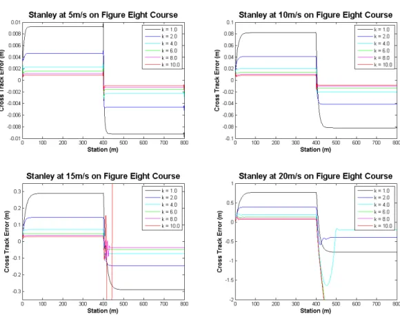
Experiments are conducted on the Figure Eight Course. Figure 16 illustrates the effects of the tuning parameter on tracking performance during these experiments. In this case, a similar dynamic effect compensation from increasing

Figure 16: Stanley controller at multiple speeds and various gains on the figure eight course

the gain as in the Pure Pursuit test is seen, so care must be taken not to over tune to a course. Additionally, it is clear that the Stanley method has some trouble with the discontinuity of the path. This may not be a problem in practice since one can guarantee smooth planned paths.

(24)

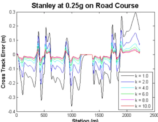
Experiments are conducted on the Road Course. Figure 17 illustrates the effects of the tuning parameter on tracking performance during these experiments. It is clear that this method works quite well under varying normal

Figure 17: Stanley controller at multiple velocity profiles and various gains on the road course

driving scenarios. The final test illustrates that this method is well suited for higher speed driving when compared to Pure Pursuit.

(25)

3 Path Tracking Using a Kinematic Model

Simplifying the vehicle system model to a kinematic bicycle model is a common approximation used for robot motion planning, simple vehicle analysis and (as for the geometric methods) deriving intuitive control laws. This chapter presents the kinematic equations of motion for such a model. In addition, an important method from control theory for chained systems is applied to reformulate the equations of motion and provide a solution to the path tracking problem. The application of this theory results in the ability to use well known control theory tools for the design of controllers and stability analysis.

3.1 Kinematic Bicycle Model

Figure 18: Kinematic bicycle model

The equations of motion for the kinematic bicycle model of a car is readily available in the literature [5, 11, 6, 4]. A derivation of the model is included here for completeness. The kinematic bicycle model collapses the left and right wheels into a pair of single wheels at the center of the front and rear axles as shown in Figure 18. The wheels are assumed to have no lateral slip and only the front wheel is steerable. Restricting the model to motion in a plane, the nonholonomic constraint equations for the front and rear wheels are:

˙

xfsin(θ+δ)−y˙fcos(θ+δ) = 0 (6)

˙

(26)

where(x, y)is the global coordinate of the rear wheel,(xf, yf)is the global coordinate of the front wheel,θis the

orientation of the vehicle in the global frame, andδis the steering angle in the body frame. As the front wheel is located at distanceLfrom the rear wheel along the orientation of the vehicle,(xf, yf)may be expressed as:

xf =x+Lcos(θ)

yf =y+Lsin(θ)

Eliminating(xf, yf)from Eq. 6:

0 = d(x+Lcos(θ))

dt sin(θ+δ)−

d(y+Lsin(θ))

dt cos(θ+δ)

= ( ˙x−θL˙ sin(θ)) sin(θ+δ)−( ˙y+ ˙θLcos(θ)) cos(θ+δ)

= ˙xsin(θ+δ)−y˙cos(θ+δ)

−θL˙ sin(θ)(sin(θ) cos(δ) + cos(θ) sin(δ))

−θL˙ cos(θ)(cos(θ) cos(δ)−sin(θ) sin(δ))

= ˙xsin(θ+δ)−y˙cos(θ+δ)

−θL˙ sin2(θ) cos(δ)−θL˙ cos2(θ) cos(δ)

−θL˙ sin(θ) cos(θ) sin(δ) + ˙θLcos(θ) sin(θ) sin(δ)

= ˙xsin(θ+δ)−y˙cos(θ+δ)−θL˙ (sin2(θ) + cos2(θ)) cos(δ)

= ˙xsin(θ+δ)−y˙cos(θ+δ)−θL˙ cos(δ)

The nonholonomic constraint on the rear wheel, Eq. 7, is satisfied byx˙ = cos(θ)andy˙ = sin(θ)and any scalar multiple thereof. This scalar corresponds to the longitudinal velocityv, such that

˙

x=vcos(θ) (8)

˙

y=vsin(θ). (9)

Applying this to the constraint on the front wheel, Eq. 6, yields a solution forθ˙

˙

(27)

−vsin(θ)(cos(θ) cos(δ)−sin(θ) sin(δ)) Lcos(δ) = v(cos 2₍_θ_{) + sin}2₍_θ_{)) sin(}_δ₎ Lcos(δ) = vtan(δ) L (10)

The instantaneous radius of curvatureRof the vehicle determined fromvandθ˙leads to the previously introduced Eq. 1: R=v_˙ θ vtan(δ) L = v R tan(δ) = L R

For the purpose of control it is useful to write the kinematic model from Eqs. 8, 9 and 10 in the two-input driftless form            ˙ x ˙ y ˙ θ ˙ δ            =            cos (θ) sin (θ) _tan( δ) L 0            v+            0 0 0 1            ˙ δ, (11)

wherevandδ˙are the longitudinal velocity and the angular velocity of the steered wheel respectively.

3.1.1 Path Coordinates

For path tracking, it is useful to express the bicycle model with respect to the path as in [6]. Defining the path as a function of its lengths, letθp(s)denote the angle between the path tangent atsand the globalxaxis. Orientation

errorθeof the vehicle with respect to the path is defined as

θe=θ−θp(s).

The curvature along the path is defined as

κ(s) =eraθp(s)

(28)

Figure 19: Kinematic bicycle model in path coordinates Multiplying both sides bys˙

˙

θp(s) =κ(s) ˙s.

Giveneraas the orthogonal distance from the center of the rear axle to the path,s˙ande˙raare

˙

s=v1cos (θe) + ˙θpera

˙

era =v1sin (θe).

Substituting(s, era, θe)for(x, y, θ)in Eq. 11 defines the kinematic model in path coordinates as

           ˙ s ˙ era ˙ θe ˙ δ            =            _cos(_θ e) 1−e˙raκ(s) sin (θe) _tan(_δ₎ L − κ(s) cos(θe) 1−e˙raκ(s) 0            v+            0 0 0 1            ˙ δ. (12)

Figure 19 illustrates the kinematic model in path coordinates.

(29)

of wheeled mobile robots and is easily extended to controlntrailers attached to the system. This section repeats the controller design found in [6] using nomenclature that is consistent with this paper for completeness.

3.2.1 Chained Form

Canonical forms for kinematic models of nonhololonomic systems are commonly used in controller design. One of these canonical structures is the chained form. The general two-input driftless control system

˙ x1=u1 (13) ˙ x2=u2 ˙ x3=x2u1 .. . ˙ xn=xn−1u1

is called(2, n)single-chained form. It turns out that this type of nonlinear chained system has a strong underlying linear structure. This linear structure allows a designer to take advantage of some well known tools in control theory. The underlying linear structure clearly appears whenu1is assigned as a function of time, and is not considered as a control variable. Under these circumstances, system 13 becomes a single-input, time-varying, linear system that has been shown to be controllable.

The conditions for converting a two-input system like 13 into chained form have been given in [9]. This conversion consists of a change of coordinatesx=φ(q), and an invertible input transformationv =β(q)u. It has been shown that this conversion can always be done successfully for nonholonomic systems withm= 2inputs andn= 3or 4 generalized coordinates. The kinematic model 12 can be put in chained canonical form by using the following change of coordinates x1=s x2=−κ ′ (s)eratan (θe)−κ(s)(1−eraκ(s)) 1 + sin2(θe) cos2₍_θ e) +(1−eraκ(s)) 2_{tan (}_δ₎ Lcos3₍_θ e) x3= (1−eraκ(s)) tan (θe) x4=era

with the input transformation

v= 1−eraκ(s) cos (θ ) u1

(30)

˙

δ=α2(u2−α1u1)

whereα1andα2are defined as

α1= ∂x2 ∂s + ∂x2 ∂era (1−eraκ(s)) tan (θe) + ∂x2 ∂θe _tan(_δ₎₍₁₋_e raκ(s)) Lcos(θe) −κ(s) α2= Lcos3₍_θ e) cos2(δ) (1−eraκ(s))2 3.2.2 Smooth Time-Varying Feedback Control

The following smooth feedback stabilization method was originally proposed in [13] and its application to vehicle path tracking was further developed in [6]. This method takes advantage of the internal structure of chained systems so as to break the solution into two design phases. The first phase assumes that one control input (that satisfies some technical requirements) is given, while the additional control input is used to stabilize the remaining sub-vector of the system state. The second phase simply consists of specifying the first control input so as to guarantee convergence while maintaining stability.

For convenience, the variables of the chained form are reordered by letting

χ= (χ1, χ2, χ3, χ4) = (x1, x4, x3, x2)

so that the chained form system can be written as

˙ χ1=u1 (14) ˙ χ2=χ3u1 ˙ χ3=χ4u1 ˙ χ4=u2

The reordering exchanges x2 andx4 so the position of the rear axle is (χ1, χ2). Now letχ = (χ1, χ2), where

(31)

3.2.3 Input Scaling

Ifu1is assigned as a function of time, the chained system 14 can be written as

˙˜ χ1= 0 (15) ˙ χ2=        0 u1(t) 0 0 0 u1(t) 0 0 0        χ2+        0 0 1        u2, with ˜ χ1=χ1− Z t 0 u1(t)dt.

The first equation in 15 is not controllable whenu1is assigned a priori. However, the structure of the differential equations forχ2is interesting. This structure looks like the familiar controllable canonical form for linear systems. Another interesting observation is that system 15 becomes time-invariant whenu1is constant and nonzero. Under this condition, the second part of system 15 becomes controllable. More importantly, it will always be controllable wheneveru1(t)is a piecewise-continuous, bounded, and strictly positive (or negative) function. Under these assump-tions,x1varies monotonically with time and differentiation with respect to time can be replaced by differentiation with respect toχ1, meaning

d dt = d dχ1χ˙1= d dχ1u1, and thus sign(u1) d dχ1 = 1 |u1| · d dt.

This change of variable is equivalent to an input scaling procedure [6]. This allows the second part to be rewritten as

χ[1]2 =sign(u1)χ3 (16)

χ[1]₃ =sign(u1)χ4

χ[1]4 =sign(u1)u′2, with the definitions

χ[_ij] =sign(u1)

dj_χ i

(32)

and u′ 2= u2 u1 .

System 16 is linear and time-invariant. It has an equivalent input-output representation of

χ[n−1]

2 =sign(u1)n−1u′2.

Such a system is controllable and admits an exponentially stable linear feedback in the form

u′ 2(χ2) =−sign(u1)n−1 n−1 X i=1 kiχ [i−1] 2 , (17)

where the gainski>0are chosen so as to satisfy the Hurwitz stability criterion. Hence, the time-varying control

u2(χ2, t) =u1(t)u′2(χ2) globally asymptotically stabilizes the originχ2= 0.

This approach leads to a solution to the path tracking problem for Ackerman steered vehicles. By transforming system 11 into path coordinates and reordering the variables as shown,χ1represents the arc lengthsalong the path,

χ2is the distanceerabetween the center of the rear axle and the path, whileχ3andχ4are related to the steering angle

δand to the relative orientationθebetween the path and the vehicle. Path tracking consists of zeroing theχ2,χ3and

χ4states independently fromχ1. Then, for any piecewise-continuous, bounded, and strictly positive (or negative)u1, equation 17 can be written as

u′

2(χ2, χ3, χ4) =−sign(u1)[k1χ2+k2sign(u1)χ3+k3χ4]. (18) Using equation 18, the final path tracking feedback control law is obtained as

u2(χ2, χ3, χ4, t) =−k1|u1(t)|χ2−k2u1(t)χ3−k3|u1(t)|χ4.

3.2.4 Tuning the Kinematic Controller

(33)

k2= 3k2

k3= 3k.

This relationship gives a single gain parameter to adjust, resulting in a manageable means to appropriately tune the controller.

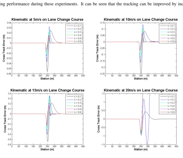
Experiments are conducted on the Lane Change Course. Figure 20 illustrates the effects of the tuning parameter on tracking performance during these experiments. It can be seen that the tracking can be improved by increasing

Figure 20: Kinematic controller at multiple speeds and various gains on the lane change course

k. The same kind of trade off between stability and performance is apparent as before. This method tracks the path accurately at low speeds, but has problems at higher speeds due to the dynamics being neglected. It can be seen that the robustness to the lane change is not as good as Pure Pursuit and is close to that of the Stanley method.

(34)

Experiments are conducted on the Figure Eight Course. Figure 21 illustrates the effects of the tuning parameter on tracking performance during these experiments. Again, it can be seen that the performance drops off as speed is

Figure 21: Kinematic controller at multiple speeds and various gains on the figure eight course

(35)

Experiments are conducted on the Road Course. Figure 22 illustrates the effects of the tuning parameter on tracking performance during these experiments. This method works quite well under varying normal driving scenarios. The

Figure 22: Kinematic controller at multiple velocity profiles and various gains on the road course

final test illustrates that this method is similar, although not as good, to the Stanley method in higher speed driving. An interesting point in the final test is that it was not the extremes of the range ofkthat was able to complete the course, rather it was in the middle.

4 Path Tracking Control Using a Dynamic Model

It is clear that neglecting vehicle dynamics in the previous models has a negative impact on tracking performance as speeds are increased and path curvature varies. The dynamics of a car are very complicated and high fidelity models are very non-linear, discontinuous and computationally expensive. This chapter derives a simple lateral dynamics model that approximates the dynamic effects and enables the design of linear path tracking controllers.

(36)

4.1 Dynamic Vehicle Model

Figure 23: Dynamic Bicycle Model

The bicycle model introduced in the last section can be extended to include dynamics. Lateral forces on the vehicle are of primary concern as path tracking is an exercise in lateral control. For this section, longitudinal velocity is assumed to be controlled separately. Summing the lateral forces illustrated in Figure 23, given vehicle massm, yields

Fyfcos (δ)−Fxfsin (δ) +Fyr=m( ˙vy+vxr). (19)

Considering only motion in the plane, a center of gravity C.G. along the center line of the vehicle, and yaw inertiaIz,

balancing the yaw moments gives

ℓf(Fyfcos (δ))−ℓr(Fyr−Fxfsin (δ)) =Izr.˙ (20)

whereris the angular rate about the yaw axis. Without the constraint on lateral slip from the last section, the slip angles of the tires are given as

αf = tan −1 _v y+ℓfr vx −δ 1 _v y−ℓrr

(37)

Modelling the force generated by the wheels as linearly proportional to the slip angle, the lateral forces are defined as

Fyf = −cfαf (21)

Fyr= −crαr.

Assuming a constant longitudinal velocity,v˙x= 0, allows the simplification

Fxf= 0. (22)

Substituting Eqs. 21 and 22 into Eqs. 19 and 20 and solving for forv˙yandr˙

˙ vy= −cf h tan−1vy+ℓfr vx −δicos (δ)−crtan−1 vy−_ℓ_r_r vx m −vxr (23) ˙ r= −ℓfcf h tan−1vy+ℓfr vx −δicos (δ) +ℓrcrtan−1 _v y−ℓrr vx Iz (24)

gives the dynamic bicycle model.

4.1.1 Linearized Dynamic Bicycle Model

To apply linear control methods to the dynamic bicycle model, the model must be linearized. Applying small angle assumptions to Eqs. 23 and 24 gives

˙ vy = −cfvy−cfℓfr mvx +cfδ m + −crvy+crℓrr mvx −vxr ˙ r=−ℓfcfvy−ℓ 2 fcfr Izvx +ℓfcfδ Iz +ℓrcrvy−ℓ 2 rcrr Izvx .

Collecting terms results in

˙ vy= −(cf+cr) mvx vy+ ₍_ℓ rcr−ℓfcf) mvx −vx r+cf mδ (25) ˙ r= ℓrcr−ℓfcf Izvx vy+ −ℓ2 fcf+ℓ2rcr Izvx r+ℓfcf m δ. (26)

(38)

Finally, the linear dynamic bicycle model can be written in state space form as    ˙ vy ˙ r   =    −(cf+cr) mvx ℓrcr−_ℓ_f_c_f mvx −vx ℓrcr−ℓfcf Izvx −(ℓ2 fcf+ℓ2rcr) Izvx       vy r   +    cf m ℓfcf m   δ. 4.1.2 Path Coordinates

Figure 24: Dynamic Bicycle Model in path coordinates

As with the kinematic bicycle model, it is useful to express the dynamic bicycle model with respect to the path. With the constant longitudinal velocity assumption, the yaw rate derived from the pathr(s)is defined as

r(s) =κ(s)vx.

Path derived lateral accelerationv˙y(s)follows as

˙

vy(s) =κ(s)v2x.

Lettingecgbe the orthogonal distance of the C.G. to the path,

¨

(39)

and

˙

ecg=vy+vxsin(θe) (28)

whereθewas previously defined asθ−θp(s). Substituting(ecg, θp)into Eqs. 25 and 26 yields

¨ ecg−vxθ˙e= −(cf+cr) mvx ( ˙ecg−vxθe) + _ℓ rcr−ℓfcf mvx −vx ( ˙θe+r(s)) + cf mδ ¨ ecg = −(cf+cr) mvx ˙ ecg+ cf+cr m θe +ℓrcr−ℓfcf mvx ˙ θe+ _ℓ rcr−ℓfcf mvx −vx r(s) +cf mδ ¨ θe+ ˙r(s) = ℓrcr−ℓfcf Izvx ( ˙ecg−vxθe) + −ℓ2 fcf+ℓ2rcr Izvx ( ˙θe+r(s)) + ℓfcf m δ ¨ θe= ℓrcr−ℓfcf Izvx ˙ ecg+ ℓfcf−ℓrcr Iz θe +− ℓ2_fcf+ℓ2rcr Izvx ( ˙θe+r(s)) + ℓfcf m δ−r˙(s).

The state space model in tracking error variables is therefore given by

           ˙ ecg ¨ ecg ˙ θe ¨ θe            =            0 1 0 0 0 −(cf+cr) mvx cf+cr m ℓfcf−_ℓ_f_c_f mvx 0 0 0 1 0 ℓrcr−ℓfcf Izvx ℓfcf−ℓrcr Iz −(ℓ2 fcf+ℓ2rcr) Izvx                       ecg ˙ ecg θe ˙ θe            (29) +            0 cf m 0 ℓfcf Iz            δ+            0 ℓrcr−ℓfcf mvx −vx 0 −(ℓ2 fcf+ℓ2rcr) Izvx            r(s)

(40)

4.1.3 Model Parameter Identification

Unlike the previous models described in Chapters 2 and 3, the dynamic bicycle model has parameters that are not as convenient to directly measure. However, a workable estimate can be obtained using commonly available tools.

The measurement of the vehicle’s split mass, utilizing four scales under each wheel, is necessary to estimate the vehicle’s total mass, C.G. location and moment of inertia. The total mass of the vehicle is simply the sum of the measurements at front and rear, left and right corners.

m=mf r+mf l+mrr+mrl

Given the modelling of the front and rear wheels as a single wheel at the center of each axle, an assumption is also made that the vehicle’s mass is laterally evenly distributed. Then a useful intermediate quantity is the sum of the measurements at the front and rear,

mf =mf r+mf l

and

mr=mrr+mrl.

From this and a measurement of the wheel baseL, the location of the vehicle’s C.G., described by distancesℓfandℓr

from the front and rear axles along the center line can be estimated as

ℓf =L 1−mf m and ℓr=L 1−mr m .

The vehicle’s moment of inertia is approximated by treating the vehicle as two point masses joined by a mass-less rod. The moment of inertia for the vehicle is then given as

Iz=ℓfℓr(mf+mr)

(41)

Figure 25: Example of lateral force tire data

Figure 26: Linear approximation of the lateral force tire data

force on the tire varies. If a data sheet is used to obtain the cornering stiffness values, a constant value describing the slope in the most linear region of the data at a nominal normal force must be chosen. Figure 26 illustrates this linear approximation. Understanding this approximation is important to understanding the limitations of the dynamic bicycle model as a whole. Note that the cornering stiffness values from the dynamic bicycle model are double the value from a data sheet since the two tires are being treated as one.

If this data is not readily available, a method to estimate it is required. Starting with Eqs. 23 and 24, repeated here for convenience ˙ vy= −cf h tan−1vy+ℓfr vx −δicos (δ)−crtan−1 _v y−ℓrr vx m −vxr

(42)

˙ r= −ℓfcf h tan−1vy+ℓfr vx −δicos (δ) +ℓrcrtan−1 _v y−ℓrr vx Iz

Eq. 23 can be rewritten as

˙ vy+vxr= ₋_ℓ fr−vy mvx + δ m cαf+ _ℓ rr−vy mvx cαr (30)

and similarly Eq. 24 as

˙ r= −(ℓfvy+ℓ 2 fr Izvx +ℓfδ Iz ! cαf+ _ℓ rvy−ℓ2rr Izvx cαr (31)

Writing these equations as functions of the cornering stiffness lends itself to the formulation of a least squares problem. Assuming that v˙y andr˙ are not directly measured, and thatv andr are available, Eqs. 30 and 31 are

rewritten in a discrete form using the Euler method as

vy(k+ 1)−vy(k) +vx(k)r(k) ∆t= ₋_ℓ fr(k)−vy(k) mvx(k) +δ(k) m ∆tcαf + _ℓ rr(k)−vy(k) mvx(k) ∆tcαr r(k+ 1)−r(k) = −(ℓfvy(k) +ℓ 2 fr(k) Izvx(k) +ℓfδ(k) Iz ! ∆tcαf + _ℓ rvy(k)−ℓ2rr(k) Izvx(k) ∆tcαr

wherekis an index of the measurement set and∆tis the time between measurement sets. The least squares formula-tion then follows as

A=B    cαf cαr   , (32) where A=              vy(2)−vy(1) +vx(1)r(1) ∆t r(2)−r(1) .. . vy(n)−vy(n−1) +vx(n−1)r(n−1) ∆t             

(43)

B=                −_ℓ_f_r(1)−_v_y(1) mvx(1) + δ(1) m ∆t ℓrr(1)−vy(1) mvx(1) ∆t −(ℓfvy(1)+ℓ2fr(1) Izvx(1) + ℓfδ(1) Iz ∆t ℓrvy(1)−_ℓ2 rr(1) Izvx(1) ∆t .. . ... −_ℓ_f_r(n−1)−_v_y(n−1) mvx(n−1) + δ(n−1) m ∆t ℓrr(n−1)−vy(n−1) mvx(n−1) ∆t −(ℓfvy(n−1)+ℓ2fr(n−1) Izvx(n−1) + ℓfδ(n−1) Iz ∆t ℓrvy(n−1)−ℓ2 rr(n−1) Izvx(n−1) ∆t               

This procedure has been used and works well in practice. However, special care needs to be taken in collecting the vehicle data. The dynamics of the vehicle must be sufficiently excited. The best results are obtained when the lateral force on the tires are moderate (without exciting the suspension too much) and continuously varying throughout the data collection. In [12] the effects of various frequencies for the steering input are studied in making these estimates. Other methods for obtaining these values both offline and online can be found in [12] and [20]. In addition to the above procedure, an optimization algorithm can be used to further fit the model to the available data. Using the above estimates to initialize an optimization algorithm that allows the inertia and cornering stiffness to change, minimizing the model error, can improve the identification.

4.2 Optimal Control

As derived in section 4.1.2, the state space model for the lateral dynamics [11] can be written as

˙ x=Ax+B1δ+B2r˙des where x= ecg e˙cg θe θ˙e T ,

ecgis the lateral distance from the C.G. to the path,θeis the heading error of the vehicle with respect to the path,δis

the steering angle input, andr˙desis the desired yaw rate determined from the current path curvature and vehicle speed.

The following values of vehicle parameters were identified using the procedure in section 4.1.3 and will be used for the control design:

m= 1140.0kg

Iz= 1436.24kgm2

(44)

ℓr= 1.165m

cf = 155494.663N/rad

cr= 155494.663N/rad

The eigenvalues of the open-loop matrixAare(0,−231.878,0,−231.878)T_{. The two eigenvalues at the origin reveals}

that the system is not stable and must be stabilized by feedback. The controllability matrix[B1, AB1, A2B1, A3B1] has full rank, therefore using the full state feedback law

δ=−Kx=−k1ecg−k2e˙cg−k3θe−k4θ˙e

allows the eigenvalues of the closed-loop matrix(A−B1K)to be placed at any desired location.

Rather than placing the eigenvalues manually, a discrete infinite-horizon Linear Quadratic Regulator (LQR) from optimal control theory is utilized. LetAd andBd refer to the discrete-time versions ofAandB1respectively. The discretization method used in the conversion is zero-order hold on the inputs with a sample time of 0.01s. Given that the pair(Ad, Bd)is controllable, the optimal steering command can be written as

δ∗ (k) =−Kx(k) where K= R+BTdP Bd −1 BdTP Ad,

the objective cost function to be minimized by the control is

J =

∞

X

k=0

xδ(k)Qx(k) +δ(k)Rδ(k),

whereP satisfies the matrix difference Riccati equation,

P =AT

dP Ad−ATdP Bd R+BdTP Bd

−1

BT

dP Ad+Q,

(45)

details to solving optimal control problems can be found in books such as [15] and many others. There are also many software packages available to perform the task.

4.2.1 Tuning the Optimal Controller

The tuning parameters for the LQR optimal control solution are

Q=            q1 0 0 0 0 q2 0 0 0 0 q3 0 0 0 0 q4            andRis chosen as R= 1.

The tuning is further reduced by setting

q2=q3=q4= 0

leaving a single parameter to adjust for tuning purposes. Setting these values to zero simply means that we are only weighting cross track error against control effort.

(46)

Experiments are conducted on the Lane Change Course. Figure 27 illustrates the effects of the tuning parameter on tracking performance during these experiments. Again, similar characteristics to the previous trackers can be seen

Figure 27: LQR controller at multiple speeds and various gains on the lane change course

as the gain is adjusted. Even though dynamics of the vehicle are included, this method fails the maneuver entirely at high speed. This is because information about the path is no longer included. The linear requirement for the vehicle model doesn’t allow for the non-linear path dynamics.

(47)

Experiments are conducted on the Figure Eight Course. Figure 28 illustrates the effects of the tuning parameter on tracking performance during these experiments. Similar problems with the discontinuity as the previous method are

Figure 28: LQR controller at multiple speeds and various gains on the figure eight course

present. An interesting point here is that the steady state error that was previously contributed to neglecting dynamics is still significant. Again, this is because the path dynamics are neglected.

(48)

Experiments are conducted on the Road Course. Figure 29 illustrates the effects of the tuning parameter on tracking performance during these experiments. Slightly improved performance is achieved in the first two tests, but

Figure 29: LQR at multiple velocity profiles and various gains on the road course

this method cannot complete the final test. The reason is similar to the kinematic trackers tendency to compensate for unmodeled dynamics with higher gains, only now it is the path that is unmodeled rather than the vehicle dynamics. It can be seen that in some scenarios, the path dynamics are as significant as the vehicle dynamics.

4.3 Optimal Control with Feed Forward Term

Continuing from the previous section, the state space model for the closed-loop system under state feedback is

˙

(49)

Since theB2r˙desterm is present, the states will not all converge to zero while the vehicle is following a constant

curvature path, despite the fact that(A−B1K)is asymptotically stable. In this section, the use of a feed forward term in addition to state feedback to ensure zero steady state error is presented. This is the method used for zeroing steady state error in [11]. Start by assuming the existence of a modified control law of the form

δ=−Kx+δf f.

Then, the closed-loop system can be written as

˙

x= (A−B1K)x+B1δf f+B2r˙des.

Taking Laplace transforms, assuming zero initial conditions, results in

X(s) = [sI−(A−B1K)]−1{B1L(δf f) +B2L( ˙rdes)},

whereL(δf f)andL( ˙rdes)are Laplace transforms ofδf f andr˙desrespectively. If the vehicle travels at a constant

speedvxon a road with constant radius of curvatureR, then

˙

rdes= constant =

vx

R

and its Laplace transform is vx

Rs. Similarly, if the feed forward term is constant, then its Laplace transform is δf f

s .

Using the Final Value Theorem, the steady state tracking error is given by

xss= lim t→∞x(t) = lim_s→0sX(s) =−(A−B1K) −1_{_B 1δss+B2 vx R}. (33)

Evaluation of equation 33 yields the steady state errors

xss=            δf f k1 0 0 0            +            −_k1 1 mv2 x R(ℓf+ℓr) ℓr 2cαf − ℓf 2cαr + ℓf 2cαrk3 −_k1 1R(ℓf+ℓr−ℓrk3) 0 1 2Rcαr(ℓf+ℓr) −2cαrℓfℓr−2cαrℓ 2 r+ℓfmvx2 0            . (34)

(50)

From equation 34, it is clear that the lateral position errorecgcan be made zero by appropriate choice ofδf f. However,

δf fcannot influence the steady state yaw error, as seen from equation 34. The yaw angle error has a steady state term

that cannot be corrected, no matter how the feed forward steering angle is chosen. The steady state yaw angle error is

θe ss= 1 2Rcαr(ℓf+ℓr) −2cαrℓfℓr−2cαrℓ2r+ℓfmvx2 θe ss=− ℓr R + ℓf 2cαr(ℓf+ℓr) mv2 x R .

The steady state lateral position error can be made zero if the feedforward steering angle is chosen as

δf f = mv2 x RL _ℓ r 2cαf − ℓf 2cαr + ℓf 2cαr k3 +L R − ℓr Rk3

which upon closer inspection is seen to be

δf f = L R +Kvay−k3 ℓr R − ℓf 2cαr mv2 x RL , where Kv= ℓrm 2cαf(ℓf+ℓr) − ℓfm 2cαr(ℓf+ℓr)

is called the understeer gradient anday = v

2

x

R. Denotingmr =mℓLf as the portion of the vehicle mass carried on the

rear axle andmf =mℓ_Lr as the portion of the vehicle mass carried on the front axle,Kv =₂m_c_αff −₂m_c_αrr . Hence

δf f =

L

R+Kvay+k3e2ss.

The steady state steering angle for zero lateral position error is given by

δss =δf f−Kxss

δss=δf f−k3θe ss

δss=

L

(51)

4.3.1 Tuning the Optimal Controller with Feed Forward Term

Experiments are conducted on the Lane Change Course. Figure 30 illustrates the effects of the tuning parameter on tracking performance during these experiments. This method improves performance over the standard LQR method.

Figure 30: LQR controller with feed forward term at multiple speeds and various gains on the lane change course Tuning in identical to that of the LQR method with the exception that the gain values are much lower. The higher gain in the LQR method can be attributed to the gain compensation from not having path dynamics.

(52)

Experiments are conducted on the Figure Eight Course. Figure 31 illustrates the effects of the tuning parameter on tracking performance during these experiments. This method greatly improves the steady state error. However, the

Figure 31: LQR controller with feed forward term at multiple speeds and various gains on the figure eight course response to the discontinuity is worse. The overshooting of the LQR with a feed forward term can be attributed to the fact that there is no look-ahead down the path in front of the vehicle. The feed forward term can only be reactive. As a result, the final test is complete failure.

(53)

Figure 32: LQR controller with feed forward term at multiple velocity profiles and various gains on the road course

Under varying normal driving scenarios, this method can perform very well when compared to the other methods.

4.4 Optimal Preview Control

To address the overshooting problem from the previous section, a preview of the path ahead of the vehicle is considered. This section presents the application of optimal linear preview control theory to vehicle steering control found in [14]. Another interesting application can be found in [10] as well. As before, the linear dynamic bicycle model is translated to the discrete time-form resulting in the state space form

xv(k+ 1) =Avxv(k) +Bvδ(k)

(54)

and the lateral profile of the path is considered in discrete sample value form, with sample values from past observations of the path ahead being stored as states of the full vehicle/path system. As the system moves forward in time, a new path sample value is read in and the oldest stored value is discarded, corresponding to the vehicle having passed the point on the path to which the oldest value refers. All the other path sample values are shifted through the time step, nearer to the vehicle. The dynamics of this shift register process are represented mathematically by

yr(k+ 1) =Aryr(k) +Bryri(k),

whereAris of the form

               0 1 0 · · · 0 0 0 1 · · · 0 .. . ... ... . .. ... 0 0 0 · · · 1 0 0 0 · · · 0               

andBris of the form

               0 0 0 .. . 1                .

Combining vehicle and road equations together, the full dynamic system can be written as

   xv(k+ 1) yr(k+ 1)   =    Av 0 0 Ar       xv(k) yr(k)   +    Bv 0   δ(k) +    0 Br   yri(k).

The complete problem is now in standard form,

(55)

Ifyriis a sample from a white noise random sequence, the time-invariant optimal control minimizing a cost function

J, given that the pair(A, B)is stabilizable and the pair(A, C)is detectable, is

u∗

(k) =−Kz(k)

with

K= R+BT_{P B}−1

BT_{P A,}

where the objective function to be minimized by the control,

J =

∞

X

k=0

zT(k)Qz(k) +δ(k)Rδ(k)

andP satisfies the matrix difference Riccati equation,

P =ATP A−ATP B R+BTP B−1

BTP A+Q,

where Q = CT_qC_{, containing the diagonal matrix,} _diag_[_q

1q2. . . qn], with terms corresponding to the number of

performance aspects contributing to the cost function, andR, corresponding to the control input, steering angle. Once formulated in this way, the same LQR problem from section 4.3 can be solved to obtain the control law and the same tuning method can be used.

(56)

4.4.1 Tuning the Optimal Preview Controller

Experiments are conducted on the Lane Change Course with a variety of preview distances. Figures 33-36 illustrate the effects of the tuning parameter on tracking performance during these experiments.

Figure 33: Optimal preview controller with 0.5s preview at multiple speeds and various gains on the lane change course

(57)

(58)

(59)

(60)

Experiments are conducted on the Figure Eight Course with a variety of preview distances. Figures 37-40 illustrate the effects of the tuning parameter on tracking performance during these experiments.

(61)

(62)

(63)

(64)

Experiments are conducted on the Road Course with a variety of preview distances. Figures 41-44 illustrate the effects of the tuning parameter on tracking performance during these experiments.

(65)

(66)

(67)

(68)

5 Performance Comparison

5.1 Tracking Results

Experiments are conducted on the Lane Change Course. Figure 45 illustrates the tracking performance of the tuned controllers during these experiments.

(69)

Experiments are conducted on the Figure Eight Course. Figure 46 illustrates the tracking performance of the tuned controllers during these experiments.

(70)

Experiments are conducted on the Road Course. Figure 47 illustrates the tracking performance of the tuned controllers during these experiments.

(71)

An empirical comparison of the path tracking methods can be found in Figure 48. It can be seen that no method is perfect and all of the methods can work well in some applications. Figure 48 lists applications that each method may be well suited for. Chapter 6 discusses this comparison in more detail.

(72)

6 Conclusions and Future Work

This research derives, implements, tunes and compares selected path tracking methods. All of the methods pre-sented are imperfect solutions in some way, but even the simplest methods can perform quite well in some common scenarios. The importance of modeling vehicle and path dynamics is highlighted as vehicle speed is increased and paths become more varying. This paper shows the varying levels of precision, complexity, implementation ease, path requirements and robustness associated with these path tracking methods. The characteristics of these trackers are often complementary and no one tracker is right for every application. Some applications may even benefit from a combination of approaches. Therefore, the understanding to be gained is the level of precision and boundaries of performance to expect from the presented methods as well as the strengths and shortcomings of using the various system models for a variety of applications. This understanding can guide selection of tracking methods for a specific application. The remainder of this chapter summarizes the characteristics of the presented system models and path tracking algorithms. A discussion of future work is also included.

Since a very detailed vehicle model can be difficult to obtain and use, the tracking methods described in this paper make use of system models that approximate vehicle motion. The approximations, simplifications, and linearization of these models vary and one needs to be aware of these shortcuts and the circumstances for which each model provides a reasonable approximation of vehicle motion. A simple kinematic model can suffice when a vehicle closely exhibits kinematic motion, such as driving slowly or performing parking maneuvers. The non-linearity of the steering angle is captured in tight turning scenarios with the kinematic model and the dynamic effects on the vehicle are minimal when driving slowly. A simple dynamic model can suffice in highway driving conditions or when the vehicle is driving at moderate speeds on smoothly varying roads. The dynamics are reasonably approximated for many driving scenarios with this model, but the model starts to break down at very slow speeds and/or tight steering angles such as parking maneuvers. These break downs in the model can be attributed to the velocity being in the denominator in the equations of motion and the linearization about the forward direction with small angle theory applied to the steering angle equation. Additionally, the model starts to break down if vehicle speed is too high on a road that is not straight. This comes from the approximation that the tire dynamics can be represented by a single value describing the ratio between lateral force and slip angle as well as another small angle approximation applied to the side slip equation. This value only represents the tire dynamics in a somewhat linear region of this non-linear function and for a small region of normal force on the tire. Higher speed cornering places the tires in the non-linear dynamics region and causes the suspension to dramatically change the normal force on the tires. The simple dynamic model also requires

(73)

described in Section 4.1.3.

Geometric path trackers are simple to understand and implement. The geometric methods presented here achieve the majority of the path tracking performance demonstrated by the other trackers until speeds are significantly in-creased. These methods include information about the path through a look-ahead distance or considering the path heading, therefore the shape of the path does not influence their performance significantly when operating at low speeds. Pure Pursuit works fairly well and is quite robust to large errors and discontinuous paths. However, it is not clear how to pick the best look-ahead distance. Varying the look-ahead distance with speed is a common approach and is the approach taken in this paper, but it makes sense that the look-ahead distance could be a function of path curvature and maybe even cross track error in addition to longitudinal velocity. Care should be taken to prevent over tuning Pure Pursuit to a specific course since changing the look-ahead distance simply changes the radius of curvature that the vehicle will travel and therefore can compensate for the increased (compared to the kinematic bicycle model prediction) radius that results from the understeer gradient of the vehicle. If tuned to insure stability, performance can be greatly reduced by cutting corners on the path due to a longer look-ahead distance. Steady state error in curves also becomes a problem as speed increases. The Stanley method is the simplest method presented and performs surpris-ingly well. In general, this method outperforms Pure Pursuit in most scenarios. However, the Stanley method is not as robust to large errors and non-smooth paths. This method is more intuitive to tune when compared to Pure Pursuit, but it suffers from similar pitfalls when tuning. The Stanley tracker can be over-tuned to a specific course in a similar manner because the only way it can overcome dynamic effects is with a high gain that may lead to instability on other paths. In contrast to Pure Pursuit, a well tuned Stanley tracker will not ”cut corners” but rather overshoot turns. This effect can be attributed to not having a look-ahead. Similar to the Pure Pursuit method, steady state errors in curves at moderate speeds become significant.

The kinematic controller presented is a little more difficult to understand and implement than the geometric meth-ods. There is a significant, yet manageable, increase in the on-line computational work needed to compute the steering angle velocity. The added complexity of this method increases the chance of making implementation mistakes. An advantage of the kinematic method is that it is easily extended for applications that need to pull a path following trailer. In fact, this method is capable of controlling multiple trailers being pulled by the vehicle. Additionally, this method can be applied to a large class of mobile robots approximated by kinematic models written in chained form. For the car-like robot application, the overall tracking performance and robustness at moderate speed is comparable to the Stanley method. Tuning the three parameters of the resulting control law in the kinematic controller is not as straight forward as the geometric methods, however a relationship between the gains reducing them to a single intu-itive parameter was given. This kinematic method requires the curvature of the path and its first two derivatives in