STANDARDIZEDhybrid video coding systems such as

Video Coding With Low-Complexity Directional

Adaptive Interpolation Filters

Dmytro Rusanovskyy, Kemal Ugur, Antti Hallapuro, Jani Lainema, and Moncef Gabbouj

Abstract— A novel adaptive interpolation filter structure for video coding with motion-compensated prediction is presented in this letter. The proposed scheme uses an independent di-rectional adaptive interpolation filter for each sub-pixel loca-tion. The Wiener interpolation filter coefficients are computed analytically for each inter-coded frame at the encoder side and transmitted to the decoder. Experimental results show that the proposed method achieves up to 1.1 dB coding gain and a 15% average bit-rate reduction for high-resolution video materials compared to the standard nonadaptive interpola-tion scheme of H.264/AVC, while requiring 36% fewer arith-metic operations for interpolation. The proposed interpolation can be implemented in exactly 16-bit arithmetic, thus it can have important use-cases in mobile multimedia environments where the computational resources are severely constrained.

Index Terms— Adaptive filters, interpolation,

motion-compensation, video coding.

I. INTRODUCTION

S

the recent H.264/AVC coding scheme [1] as well as older standards, e.g., MPEG-1, 2, 4, H.262, and H.263, are all based on motion-compensated prediction. The state-of-the art video coding standard H.264/AVC supports state-of-the use of motion vectors with quarter pixel accuracy for motion-compensated prediction. The fractional-pixel samples are ob-tained using a six-tap Wiener filter that is designed to minimize the adverse affects of aliasing [2]. However, aliasing in a video sequence is not a stationary process but has vary-ing characteristics. Adaptive interpolation filters that change the filter coefficients at each frame have been proposed in the literature to overcome this nonstationary effect of aliasing and thus increase the coding efficiency of video codecs [3], [4].

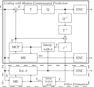
Fig. 1 shows a generalized block diagram of a hybrid video encoder with adaptive interpolation filters. The up-per blocks of the diagram enclosed within a solid thick

Manuscript received January 16, 2008; revised October 21, 2008; accepted December 5, 2008. First version published May 12, 2009; current version published August 14, 2009. This work was supported by the Nokia Research Center and by the Academy of Finland, Application Number 213462, Finnish Programme for Centers of Excellence in Research 2006–2011. This paper was recommended by Associate Editor S. Li.

D. Rusanovskyy and M. Gabbouj are with the Department of Signal Processing at Tampere University of Technology, 33720 Tampere, Finland (e-mail: [email protected]; [email protected]).

K. Ugur, A. Hallapuro, and J. Lainema are with the Nokia Research Center, Nokia Corporation, 33720 Tampere, Finland (e-mail: [email protected]; [email protected]; [email protected]).

Digital Object Identifier 10.1109/TCSVT.2009.2022708

line rectangle represent a conventional encoder structure with fractional-pixel motion-compensated prediction, e.g., H.264/AVC, while those enclosed within a dash-dotted rec-tangle depict the estimation process of the interpolation filter.

In hybrid video coding scheme, the current image X is to be predicted by motion-compensated prediction (MCP) from the already encoded reference image Y. The result of the motion-compensated prediction is the predicted imageX. The prediction error E is undergoing the transform coding (T) and quantization (Q) following the entropy encoding (ENC). In addition to encoding the prediction error E, the motion informationmvthat is obtained by the motion estimation (ME) is coded and transmitted to the decoder side.

Video coding with adaptive interpolation assumes that coef-ficients of the interpolation filterhare computed for each inter-predicted frame, and this process is shown in Fig. 1 within the dash-dotted block. The adaptive filterh is the optimal Wiener filter minimizing the error energy of the motion-compensated prediction.

In [4], Vatis et al. proposed a 2-D nonseparable adap-tive interpolation filter (2-D-AIF). For each sub-pixel posi-tion, this scheme utilizes an independent 2-D nonseparable filter size of 6 ×6 tap. A total of 36 filter coefficients for each filter are calculated by minimizing the prediction error energy of each coded frame. It was reported that coding gains of up to 1.1 dB are achieved over the stan-dard H.264/AVC especially at high-resolution high-quality videos. However, the improvement in the coding efficiency with 2-D-AIF scheme comes at the expense of having ap-proximately three times higher interpolation complexity com-pared to the standard H.264/AVC [5]. The reasons for such increase are the nonseparable nature of 36-tap filters and the need to perform operations in 32-bit arithmetic. Since interpolation is already one of the most complex parts of H.264/AVC decoders [6], a further increase in the complex-ity is very problematic, especially for resource-constrained devices, such as portable video players or recorders.

In this letter, we propose a novel adaptive Wiener interpola-tion scheme to improve the coding efficiency of video coders, with significantly less complexity than its counterparts [4]. The proposed method uses directional filters to interpolate each sub-pixel sample. The direction of the interpolation filter for each sub-pixel position is determined based on the alignment of the corresponding sub-pixel with integer-pixel samples. The proposed filter structure allows the use of 16-bit integer opera-tions at the decoder, thus providing a very low computational

mv

Coding with Motion-Compensated Prediction T

MCP

ENC

ENC

Filter Estimation Y Yavc ME Est. h Q ENC Interp. with h Interp. H.264/ AVC Y Q–1 T–1 z–1 E’ + + – X X X’ ME

Fig. 1. Block diagram of a hybrid video encoder based on motion-compensated prediction with adaptive interpolation filter.

complexity of interpolation at the decoder. Since significant coding efficiency is achieved with low decoding complexity, it is believed that the proposed method has important use-cases in mobile multimedia environments where the computational resources are severely constrained.

This letter is organized as follows. The proposed filter architecture is given in Section II. In Section III we dis-cuss the interpolation process, describe its integer imple-mentation, and provide its complexity estimates. Section IV presents simulation results, while Section V concludes the letter.

II. PROPOSEDFILTERSTRUCTURE

Consider Fig. 2, where the pixel locations in the original im-age grid (we call them integer-pixels locations) are labeled by upper case letters {A1, . . . ,F6}within the shaded boxes, and lower case symbols {a,b, . . . ,o} represent locations of sam-ples at sub-pixel image grid (sub-pixel locations) that are to be interpolated. The proposed algorithm uses a single directional adaptive interpolation filter (DAIF) to generate each sub-pixel. Let us denote an interpolation filter used for each sub-pixel

Sp, Sp ∈ {a,b, . . . ,o}, with h(Sp). The direction of these filters is determined according to the alignment of the corre-sponding sub-pixelSpwith the integer-pixels. Such sub-pixel-specific filter alignment leads to different sets of integer-pixels, which are used to estimate the filter h(Sp) and interpolate

Sp-sample. We denote these sets as s(Sp) ⊆ {A1, . . . ,F6}. The following describes the alignment of the filters’ directions and therefores(Sp)in detail.

A. Alignment of Filters’ Directions

Sub-pixel locations{a,b,c}and{d,h,l}are horizontally and vertically aligned with samples at integer locationss(a|b|c)=

{C1,C2, . . . ,C6} and s(d|h|l) = {A3,B3, . . . ,F3}, respec-tively, as it shown in the Fig. 2(a). Therefore, only those image samples at the respectives(Sp)locations are utilized for filter

h(Sp)estimation and interpolating of {a,b,c}and{d,h,l}.

res1 res1 res2 res2 A1 A2 A3 A4 A5 A6 B1 B3 B4 B5 B6 C1 C2 C3 C4 C5 C6 D1 D2 D3 D4 D5 D6 E1 E2 E3 E5 E6 F1 F2 F3 F4 F5 F6 a bc e f g i j k m d h l no res4 res3 res2 res1 A2 A3 A4 A5 A6 A1 B2 B3 B4 B5 B6 B1 C2 B3 C4 C5 C6 C1 D2 D3 D4 D5 D6 D1 E2 E3 E4 E5 E6 E1 F2 F3 F4 F5 F6 F1 a bc e f g i j k m d h l no (a) (b)

Fig. 2. Interpolation process; (a) two partial sums (res1 andres2) required for each of{a,b,c,d,h,k}and (b) four partial sums for{f,i,j,k,n}.

Sub-pixel locationse,oare diagonally aligned with integer-pixels in the northwest–southeast direction, whereas for locations g,m such alignment is in northeast–southwest direction, see Fig. 2(b). Therefore, image samples at coordinates s(e|o)= {A1,B2,C3,D4,E5,F6} ands(g|m)=

{A6,B5,C4,D3,E2,F1} are used for interpolating sub-pixel locations {e,o} and {g,m}, respectively. Locations

{f,i,j,k,n} are either aligned with integer-pixel samples in both diagonal directions (location j), or have no integer-pixel samples to be aligned with (positions f,i,k,n). For this reason, {f,i,j,k,n} are interpolated using the integer-pixels that lie on a diagonal cross structure{A1,B2, . . . ,F6} ∪

{F1,E2, . . . ,A6}. The sets of integer-pixel locations that contribute to the interpolation at each sub-pixel location are denoted withs(Sp)and are given explicitly as following:

s(a)=s(b)=s(c)= {C1,C2,C3,C4,C5,C6} s(d)=s(h)=s(l)= {A3,B3,C3,D3,E3,F3} s(e)=s(o)= {A1,B2,C3,D4,E5,F6} s(m)=s(g)= {F1,E2,D3,C4,B5,A6} s(j)=s(f)=s(i)=s(k)=s(n)= {A1,B2,C3,D4,E5,F6,F1,E2,D3,C4,B5,A6}. (1)

B. Calculatingthe Filter Coefficients

The interpolation filter estimation diagram is depicted in Fig. 1 within a dash-dotted block. The filter coefficients are analytically calculated for every P- or B-coded frame X. First, initial motion vectorsmvwith 1/4-pixel accuracy are found by performing motion estimation with the standard H.264/AVC interpolation (Yavc). Using this motion information, filters

h(Sp) are calculated by solving a system of Wiener–Hopf equations [7], which are constructed fromYavcand X images independently for each Sp. Coordinates of image samples which are used for h(Sp) estimations are given in (1) as

s(Sp) in terms of relative (local coordinates) {A1, . . . ,F6}. The link between these relative coordinates and the absolute image coordinates(x,y)can be established as follows.

Consider a sample Xx_,y located at the (x,y) coordinate

in the original video frame X. Its local neighborhood with a size of 6×6 pixels is shown in Fig. 2 as {A1, . . . ,F6}x_,y,

whereasXx,y is associated with C3 position. The sampleXx,y

is predicted from the reference imageYavcwith motion vector

mvx,y = (d x,d y). The integer part of this motion vector

mvx,y

of C3 position in the up-sampled reference frame Yavc as (4x+4· d x,4y+4· d y). The absolute coordinates of

{A1, . . . ,F6}x_,y positions in Yavccan be derived accordingly.

The fractional component of the current mvx,y determines a

sub-pixel locationSp∈ {a,b, . . . ,o}and hence the interpola-tion filterh(Sp)which is to be computed from{A1, . . . ,F6}x_,y

samples of the reference and the original images.

Filter coefficientsht(Sp), wheret is the coefficient’s index,

are calculated by solving a system of Wiener–Hopf equations. For an N-tap filter, the system of equations is given in (2)

N₋1

t=0

Rr_t−i,i(Sp)·ht(Sp)=Ricr(Sp), i,t=0, . . . ,N−1 (2)

where Rcr(Sp)and Rr(Sp)are the expected cross-covariance and auto-covariance functions computed from the original and the reference images independently for eachSp

Rcr_t (Sp)=E[Y(st(Sp))·X(C3)] (3)

Rr_t,i(Sp)=E[Y(st(Sp))·Y(si(Sp))] (4)

wheres(Sp)is a set of integer-pixels locations given in (1). A practical approach to compute expectations (3) and (4) is to average local covariances over all motion vectors which were estimated fromYavc.

III. INTERPOLATIONPROCESS

After the adaptive filter coefficients are calculated, the refer-ence image samplesY are interpolated at sub-pixels locations

Sp as follows:

Y(Sp)=

N−1

t=0

Y(st(Sp))·ht(Sp). (5)

Interpolation at sub-pixel positions {a,c,d,l,e,g,m,o}is accomplished with a 6-tap filter (N = 6) and {f,i,j,k,n}

samples are interpolated with N =12, as shown in (5). And, the filter calculation process described in Section II places no restrictions on floating point filter coefficientsht.

However, in order to perform interpolation with integer arithmetic, ht should be represented by integer values with

finite word length. A signedht value is represented withQ+1

bits as follows: htQ =sign(ht)· |ht| ·2Q+0.5 (6) where Qis the number of bits representing the magnitude and the leftmost bit is reserved for the sign. Using this represen-tation, interpolation is performed using integer arithmetic as follows: Y(Sp)= _N−1 t=0 Y(st(Sp))·htQ+2Q−1 Q. (7)

Larger Q improves the accuracy of filter coefficient repre-sentation but increases the required memory size and memory-access bandwidth. In order to have the convolution sum in (7) fit in a 16-bit memory storage, the filter coefficientsht should

be represented with a maximum of 4-bit accuracy(Q=4). It was found empirically, that havingQ<8 significantly reduces the coding efficiency.

A. 16-Bit Integer Arithmetic Implementation

In order to achieve guaranteed 16-bit operation for the inter-polation operation and still keep the coding efficiency high, a filter-specific calculation structure is proposed. The proposed method exploits the typical characteristics of interpolation filters and places certain restrictions on the filter coefficient values.

The proposed structure performs interpolation not using the equation given in (7), but using partial sums as shown in Fig. 3. Two partial sums are required to interpolate Y(Sp)for Sp∈

{a,b,c,d,h,l,e,g,m,o}and they are given as

res1= ₂ t=0 Y(st(Sp))·htQ(Sp) , res2= ₅ t₌3 Y(st(Sp))·htQ(Sp) .

Two additional partial sums are required to interpolateY(Sp)

for Sp∈ {f,i,k,n,j}and these sums are given as

res3= ₈ t=6 Y(st(Sp))·hQt (Sp) , res4= ₁₁ t=9 Y(st(Sp))·htQ(Sp) .

For typical filter coefficients and image samples, positive values of partial sums prevail in observed statistics. So we can gain additional accuracy for filter coefficients by clipping the partial sums below zero, e.g., res1 =max(0,res1). Since all intermediate resultsres1,res2,res3, andres4 are positive, their representation format is converted from a signed 16-bit integer to an unsigned 16-bit integer. This allows one additional bit accuracy for defining the magnitude of the coefficients.

In order to avoid overflow and underflow and keep the partial sums fit in the signed 16-bit registers, we define two requirements on filter coefficient values

⎛ ⎝j+2 t=j max 0,htQ(Sp) <128 ⎞ ⎠ and ⎛ ⎝ j+2 t=j min 0,htQ(Sp) >−128 ⎞ ⎠

where j = 0,3 and j = 0,3,6,9 for {a,c,d,l,e,g,m,o}

and {f,i,k,n,j} filters, respectively. With these restrictions in place, Q in (6) could be set as Q=7 and the coefficients take values of −127/128,−126/128, . . . ,126/128,127/128, with accuracy 1/128. The accuracy of filter coefficients is increased from 4 bits to 7 and still guaranteeing 16-bit integer implementation.

Additional bit accuracy for filter coefficients of sub-pixel locations {f,i,k,n,j} is gained by observing the fact that the statistical distribution of those coefficients most often fall in the range [−0.5, 0.5], instead of [−1,1]. We exploit this fact and restrict the filter coefficients of sub-pixel loca-tions{f,i,k,n,j}to the range [−0.5,0.5]. More specifically,

the floating point filter coefficients of sub-pixel locations

{f,i,k,n,j} is converted to integer representation as shown in (6), with Q=8, instead of 7.

Using the filtering operation and the restrictions described above, the accuracy of the filter-coefficients is increased from 4 bits to 7 for {a,c,d,l,e,g,m,o}and to 8 for{f,i,k,n,j}

sub-pixel locations. The interpolation operations final ex-pressions (8) and (9) are given for 16-bits interpolation of

{a,c,d,l,e,g,m,o}and{f,i,k,n,j}respectively Y(Sp)= res1+res2+2Q−1 Q, for Q=7 andSp∈ {a,b,c,d,h,l,e,g,m,o} (8) Y(Sp)=

(res1+res2)1+(res3+res4)1

+2Q−2

Q−1

Q=8 andSp∈ {f,i,j,k,n}. (9) In rare cases where the coefficient calculation process (2) results in coefficients that do not fulfill the conditions given in this section, the static interpolation filter is used for the corresponding sub-pixel location.

B. Interpolation Complexity Analysis

In this section we provide complexity analysis of the in-terpolation process that should be implemented at the decoder side. The complexity of the filter estimation process is beyond the scope of this letter, as it is an encoder algorithm and has much less restriction on the complexities.

First, we estimate the interpolation complexity of the pro-posed DAIF scheme as given in (7) and compare it with the complexities of the standard H.264/AVC and the most recently proposed 2-D-AIF interpolations, which are reported in [5]. This estimation was done in terms of the number of basic arithmetic operations, such as summation, multiplication, and shift, required to interpolate each sub-pixel location. The complexity estimate for each sub-pixel as well as the average of all sub-pixels complexities are given in Table I. Analysis of Table I shows that DAIF scheme requires about 38% of the number of operations needed for 2-D-AIF to interpolate the reference image (all sub-pixel locations). Moreover, our method requires about 36% less arithmetic operations in comparison to the standard H.264/AVC interpolation. As seen in Table I, the worst case complexity (which is an important parameter for decoding complexity) of the proposed scheme is reduced by 41% compared to H.264/AVC and reduced to one-third of the 2-D-AIF scheme.

Second, we estimate the complexity of the proposed interpolation implemented with 16-bit arithmetic, as given in (8) and (9), and compare it with complexity estimates for the 16-bit implementation of the H.264/AVC interpolation, available in [5]. Estimation results are given in Table II. Analysis of Table II shows that the proposed 16-bit implementation of DAIF interpolation has a complexity that is comparable with the highly optimized H.264/AVC on average for all sub-pixels as well as in the worst case scenario. We realize that the number of arithmetic operations is a simple approximation of the complexity and does not

TABLE I

NUMBER OFARITHMETICOPERATIONSREQUIRED TOINTERPOLATE SUB-PIXELPOSITIONS

Sub-pixel position H.264/AVC [1] 2-D-AIF [4] DAIF

b,h 10 10 10

a,c,d,l 13 13 13

e,g,m,o 23 58 13

J 32.5 41 16

f,i,k,n 35.5 55 19

Average per sub-pixels 22.56 37.66 14.4 TABLE II

NUMBER OF16-BITARITHMETICOPERATIONSREQUIRED TO INTERPOLATESUB-PIXELPOSITIONSWITHIN16-BITSARITHMETIC

Sub-pixel position H.264/AVC [1] DAIF-16-bit

b,h 10 17

a,c,d,l 13 17

e,g,m,o 23 17

J 32.5 35

f,i,k,n 35.5 35

Average per sub-pixels 22.56 23 TABLE III

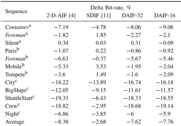
SIMULATIONRESULTS OF THE2-D-AIFANDPROPOSEDDAIF SCHEMES COMPARING TO THEH.264/AVC INTERPOLATION

Sequence Delta Bit-rate, %

2-D-AIF [4] SDIF [11] DAIF-32 DAIF-16

Containera −7.19 −4.78 −8.06 −9.06 Foremana −1.82 1.85 −2.27 −2.1 Silenta 0.34 0.03 0.31 −0.09 Parisb −1.07 0.22 −0.86 −0.92 Foremanb −6.63 −0.37 −5.67 −5.46 Mobileb −5.33 3.53 −1.95 −2.04 Tempeteb −3.6 1.49 −1.6 −2.09 Cityc −18.22 −13.89 −16.74 −16.18 BigShipsc −12.05 −9.15 −11.61 −11.57 ShuttleStartc −19.33 −6.43 −18.33 −18.55 Crewc −18.82 −2.95 −18.68 −19.14 Nightc −6.86 −3.85 −6 −5.9 Average −8.38 −2.68 −7.62 −7.76

a_{-QCIF resolution,}b_{-CIF, and}c_{-720p resolution of video sequences.}

consider computational architecture, e.g., memory bandwidth, use of parallel arithmetic, and so on. However, we believe these estimates are useful for illustration purposes.

IV. EXPERIMENTALRESULTS

Both of the proposed implementations of DAIF scheme, i.e., the 32-bit version as given in (7) with Q=8 and the 16-bit version as given in (8) and (9), were adopted for integration into the official reference ITU-T VCEG-KTA software [12].

In order to test the performance of the proposed interpo-lations, we produced rate–distortion curves with VCEG-KTA software [8] following the common test conditions defined in the ITU-T/VCEG group [9] with the baseline profile settings.

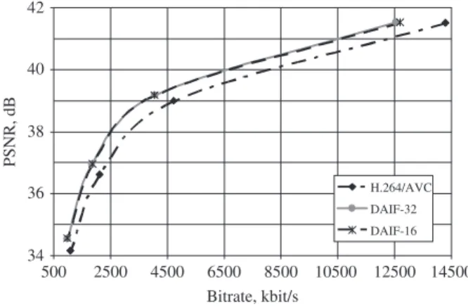
34 36 38 40 42 500 2500 4500 Bitrate, kbit/s P SNR, dB H.264/AVC DAIF-32 DAIF-16 14500 6500 8500 10500 12500

Fig. 3. Rate–distortion curves for “Crew” sequence, 60 frames/s.

34 36 38 40 42 44 400 Bitrate, kbit/s P SNR, dB H.264/AVC DAIF-32 DAIF-16 5400 4400 3400 2400 1400

Fig. 4. Rate–distortion curves for “ShuttleStart” sequence, 60 frames/s.

Simulations were performed with test video sequences at QCIF, CIF, and 720p resolutions with a total of 300 coded frames for sequences at QCIF and CIF resolutions, and 150 coded frames for video materials at 720p resolutions. The standard H.264/AVC interpolation [1] was used as an anchor, and all simulation results are presented in Table III in terms of bit-rate reduction (%) compared to the anchor. Table III provides the simulation results for two integer implementations (32-bit and 16-bit) of the proposed DAIF scheme, noted as DAIF-32 and DAIF-16. Encoded bit streams for these schemes included side information for adaptive filters such as quantized filter coefficients, and thus the generated streams were fully decodable.

Table III also illustrates the simulation results for two more interpolation schemes: the 2-D-AIF which denotes the video coding with 2-D nonseparable adaptive filters (2-D-AIF) [4]; and the SDIF which is the most recently proposed static direc-tional interpolation filtering [11]. Addidirec-tionally, rate–distortion curves achieved with the proposed DAIF scheme for “Crew” and “ShuttleStart” test sequences are given in Figs. 3 and 4 respectively.

As seen from Table III and the figures, a significant coding gain is achieved by the DAIF scheme compared to H.264/AVC. This gain comes from both the directional filter structure (SDIF outperforms the H.264/AVC interpolation by 2.7% in bit-rate reduction) and from adapting filter coefficients (∼7.7% of bit-rate reduction compared to H.264/AVC). Both DAIF schemes, the DAIF-32 and DAIF-16, provide comparable

coding gain, about −7.7% of delta bit rate on average and 15% of bit-rate reduction for 720p video material. However, DAIF-16 slightly outperforms the DAIF-32 on low-resolution video sequences. This is because of reduced number of bits needed for transmitting the filter coefficients for DAIF-16 due to the lower dynamic range of the filter.

In comparison to the 2-D-AIF, the proposed scheme achieves comparable results as well (−0.03 dB on average), with significantly lower complexity. Additionally, it should be noted that the proposed DAIF scheme achieves about 1% of bit-rate reduction over the 2-D-AIF interpolation for low-resolution video sequences (QCIF) due to the significantly re-duced bit overhead required for filter coefficients transmitting.

V. CONCLUSION

The recent H.264/AVC video coding standard supports motion-compensated prediction with up to 1/4-pixel accuracy motion vectors. In this letter, we proposed a novel interpolation scheme using DAIF for each sub-pixel location. Experimental results show that DAIF achieves about 7.7% of bit-rate reduc-tion on average and 15% for high-resolureduc-tion video compared to the standard nonadaptive interpolation scheme of H.264/AVC, while requiring 36% fewer operations for interpolation. Com-pared to the 2-D-AIF scheme, the proposed scheme has prac-tically the same coding efficiency with approximately three times less complexity. The DAIF scheme as well as its 16-bit implementation described in this letter were both applied to the ITU-T/VCEG standardization and successfully adopted in the reference VCEG-KTA software [12].

REFERENCES

[1] Recommendation ITU-T H.264 & ISO/IEC 14496-10 (MPEG-4) AVC, “Advanced Video Coding for Generic Audiovisual Services,” v.3: 2005. [2] T. Wedi and H. G. Musmann, “Motion and aliasing-compensated predic-tion for hybrid video coding,”IEEE Trans. Circuits Syst. Video Technol., vol. 13, no. 7, pp. 577–587, Jul. 2003.

[3] T. Wedi, “Adaptive interpolation filters and high-resolution displace-ments for video coding,”IEEE Trans. Circuits Syst. Video Technol., vol. 16, no. 4, pp. 484–491, Apr. 2006.

[4] Y. Vatis, B. Edler, D. T. Nguyen, and J. Ostermann, “Motion and aliasing-compensated prediction using a 2-D nonseparable adaptive wiener interpolation filter,” inProc. ICIP2005, vol. 2. Genova, Italy, Sep. 2005, pp. 894–897.

[5] Y. Vatis and J. Ostermann, “Comparison of complexity between 2-D nonseparable adaptive interpolation filter and standard wiener filter,” Nice, France, ITU-T SGI 6/Q.6 Doc. VCEG-AA11, Oct. 2005. [6] V. Lappalainen, A. Hallapuro, and T. D. H¨am¨al¨ainen, “Complexity

of optimized H.264/AVC video decoder implementation,”IEEE Trans.

Circuits Syst. Video Technol., vol. 13, no. 7, pp. 717–725, Jul. 2003.

[7] A. Papoulis,Probability, Random Variables, and StochasticProcesses. 3rd ed. New York: McGraw-Hill, 1991, ch. 13, pp. 580–629. [8] ITU-T VCEG. (2007, Aug. 7). version 1.4.

Refer-ence ITU-T VCEG-KTA Software [Online]. Available:

http://iphome.hhi.de/suehring/tml/download/

[9] T. K. Tan, G. Sullivan, and T. Wedi, “Recommended simulation common conditions for coding efficiency experiments,” Marrakech, Morocco, ITU-T Q.6/SG16, VCEG-AE010, Jan. 2007.

[10] J. K. Tungait, “Modeling and identification of symmetric noncausal impulse responses,” IEEE Trans. Acoust., Speech, Signal Process., vol. 34, no. 5, pp. 1171–1181, Oct. 1986.

[11] A. Fuldseth, G. Bjontegaard, D. Rusanovskyy, K. Ugur, and J. Lainema, “Low-complexity directional interpolation filter,” Berlin, Germany, ITU-T Q.6/SG16, VCEG-AI12, Jul. 2008.

[12] D. Rusanovskyy, K. Ugur, and J. Lainema, “Adaptive interpolation with directional filters,” Shenzhen, China, VCEG-AG21, Oct. 20, 2007.