The Study of Transition Metal Oxides using Dynamical Mean Field Theory

The Study of Transition Metal Oxides using

Dynamical Mean Field Theory

Hung The Dang

Submitted in partial fulfillment of the

Requirements for the degree

of Doctor of Philosophy

in the Graduate School of Arts and Sciences

COLUMBIA UNIVERSITY

Hung The Dang All Rights Reserved

Abstract

The Study of Transition Metal Oxides using Dynamical

Mean Field Theory

Hung The Dang

In this thesis, we study strong electron correlation in transition metal oxides. In the systems with large Coulomb interaction, especially the on-site interaction, elec-trons are much more correlated and cannot be described using traditional one-electron picture, thus the name “strongly correlated systems”. With strong correlation, there exists a variety of interesting phenomena in these systems that attract long-standing interests from both theorists and experimentalists. Transition metal oxides (TMOs) play a central role in strongly correlated systems, exhibiting many exotic phenomena. The fabrication of heterostructures of transition metal oxides opens many possible directions to control bulk properties of TMOs as well as revealing physical phases not observed in bulk systems.

Dynamical mean-field theory (DMFT) emerges as a successful numerical method to treat the strong correlation. The combination of density functional and dynamical mean-field theory (DFT+DMFT) is a prospectiveab initio approach for studying re-alistic strongly correlated materials. We use DMFT as well as DFT+DMFT methods as main approaches to study the strong correlation in these materials.

We focus on some aspects and properties of TMOs in this work. We study the magnetic properties in bulk TMOs and the possibility of enhancing the magnetic order in TMO heterostructures. We work on the metallic/insulating behaviors of these

parameters of materials. We also investigate the effect of a charged impurity to the neighborhood of a correlated material, which can be applied, for example, to the study of muon spin relaxation measurements in high-Tc superconductors.

Contents

Contents i

List of Tables iv

List of Figures v

1 Introduction 1

1.1 Transition metal oxides . . . 1

1.2 Heterostructures of transition metal oxides . . . 6

1.3 Metal-insulator transition . . . 9 1.4 Magnetism . . . 15 1.5 Charged impurity . . . 21 2 Formalism 24 2.1 General description . . . 24 2.1.1 Lattice structure . . . 25

2.1.2 General band structure for TMOs . . . 27

2.2 Models . . . 34

2.2.1 The kinetic Hamiltonian Hkin . . . 35

2.2.2 Onsite Coulomb interaction Honsite . . . 43

2.2.3 Double counting correction HDC . . . 45

2.2.4 Intersite Coulomb interaction Hcoulomb . . . 49

2.3 Dynamical mean-field theory (DMFT) . . . 50

2.3.2 Impurity solver . . . 57

2.3.3 Applications of DMFT in TMOs . . . 58

3 Ferromagnetism in early TMOs 60 3.1 Introduction . . . 60

3.2 Model and Methods. . . 64

3.2.1 Geometrical structure . . . 64

3.2.2 Electronic structure. . . 67

3.2.3 The magnetic phase boundary . . . 70

3.3 Vanadate bulk and superlattices . . . 72

3.3.1 Magnetic phase diagram . . . 72

3.3.2 The effect of oxygen bands . . . 80

3.3.3 Relation between superlattice and bulk system calculations . . 84

3.3.4 Superlattices with GdFeO3-type rotation . . . 90

3.4 Ruthenate systems CaRuO3 and SrRuO3. . . 93

3.5 Conclusions . . . 98

4 Covalency and the metal-insulator transition 101 4.1 Introduction . . . 102

4.2 Model and methods . . . 105

4.2.1 Overview . . . 105

4.2.2 Solution of correlation problem . . . 106

4.2.3 The double-counting correction and the d-level occupancy . . 108

4.3 Overview of results . . . 109

4.4 Hartree calculations for cubic structures . . . 112

4.5 DFT+DMFT calculations for cubic structures . . . 115

4.6 GdFeO3-distorted structures . . . 118

4.7 Locating materials on the phase diagrams . . . 124

4.8 Conclusions . . . 128

5 Charged impurities in correlated electron materials 131 5.1 Introduction . . . 131

5.2 Model and method . . . 134

5.2.1 Model . . . 134

5.2.2 Method . . . 137

5.3 Results: density distribution . . . 142

5.4 Results: spin correlations . . . 143

5.5 Conclusion . . . 146

Bibliography 168

A Derivation of the onsite Coulomb interaction 169

B Analytic continuation with MaxEnt method 175

C Lattice distortion 180

D Full charge self consistency effect 183

E Determine the metal-insulator transition 187

F CTQMC impurity solver 191

2.1 Tight binding parameters for some hypothetical cubic perovskites . . 39 3.1 Comparing the Curie temperatures for some cases ind-only andpdmodel 83 4.1 Values ofd occupancy for different double counting corrections . . . . 126 4.2 Experimental data for the energy gaps and the oxygenp band positions127 D.1 Summary ofdoccupancy for SrVO3 obtained from full-charge self

con-sistent calculation . . . 184

List of Figures

1.1 Transition metal elements in the periodic table . . . 2

1.2 Phase diagrams of several strongly correlated materials . . . 3

1.3 Zaanen-Sawatzky-Allen diagram . . . 4

1.4 Illustration of Mott-Hubbard and charge-transfer insulators . . . 5

1.5 Ferromagnetism in vanadium-based oxide superlattices . . . 8

1.6 “Mott behavior” in real life . . . 10

1.7 Spectral function in Mott transitions . . . 13

1.8 Schematic diagram for the MIT in TMO perovskites. . . 14

1.9 Types of magnetic order phases . . . 16

1.10 Stoner model for ferromagnetism . . . 18

1.11 Magnetic phase diagram for the Hubbard model in mean field calculation 19 1.12 Example of orbital currents in pseudogap phase . . . 22

2.1 Examples of lattice structures of TMOs . . . 25

2.2 P mnadistorted structure of perovskites . . . 26

2.3 Crystal field splittings . . . 29

2.4 Arrangements of p and d orbitals in perovskites . . . 30

2.5 Density of states for SrVO3 . . . 32

2.6 Schematic density of states with Zhang-Rice band . . . 33

2.7 Band structure of SrVO3 and energy range for each bands . . . 42

2.8 Illustration for the double counting correction . . . 47

2.9 Dynamical mean-field theory: impurity and bath . . . 52

3.1 Representation of ABO3 perovskite structure with GdFeO3-type

dis-tortion . . . 65 3.2 Schematic of superlattice lattice structure (LaVO3)m(SrVO3)1and

nearest-neighbor electron hoppings . . . 68 3.3 Extrapolate the Curie temperature from inverse magnetic susceptibility 71 3.4 Density of states for bulk LaVO3 with increasing tilt angle . . . 73

3.5 Inverse magnetic susceptibility and the Wilson ratio vs. temperature 74 3.6 Inverse susceptibility vs. temperature as tilt angle increases. . . 76 3.7 The magnetic phase diagram of bulk vanadate system as a function of

doping and tilt angle . . . 77 3.8 The dependence of Curie temperature Tc on van Hove peak position . 79

3.9 Inverse susceptibility vs. temperature for pdvs d-only model . . . 81 3.10 Comparison of inverse susceptibility vs. temperature curve for pd

model with/withouteg contribution and d-only model . . . 84

3.11 Noninteracting density of states of bulk and superlattice structure without distortion. . . 85 3.12 Inverse susceptibility vs. temperature for untilted superlattices . . . . 87 3.13 Comparison between bulk and superlattice density of states with the

same P21/m distortion . . . 88

3.14 Comparison of inverse susceptibility for bulk and superlattice with the same P21/m distorted structure . . . 90

3.15 Density of states for bulk P21/m structure with increasing tilt angle . 91

3.16 The magnetic phase diagram for P21/m structure as a function of

doping and tilt angle . . . 93 3.17 Noninteracting density of states for CaRuO3 and SrRuO3 . . . 95

3.18 The ferromagnetic/paramagnetic phase diagrams for CaRuO3and SrRuO3 96

4.1 Energy windows for MLWF projection in SrVO3 and LaNiO3 . . . 103

4.2 Compare the Matsubara self energy obtained from DMFT with Ising and rotationally invariant interactions. . . 107 4.3 Noninteracting density of states for SrVO3, LaTiO3 and YTiO3 derived

from DFT+MLWF method . . . 110 4.4 The density of states of SrVO3 at different U values obtained from

DFT+U, Hartree and DMFT . . . 112 4.5 Hartree calculation of U-dependent t2g occupancy for majority and

minority spins for SrVO3 . . . 113

4.6 Hartree phase boundaries for metal-insulator transitions for Sr and La perovskite series . . . 114 4.7 The metal-insulator phase boundaries for “cubic” La perovskite series

obtained from Hartree and DMFT. . . 116 4.8 Spectral functions for “cubic” La perovskite series at the metal-insulator

boundary . . . 118 4.9 The metal-insulator phase diagrams for “cubic” and “tilted” LaTiO3

and LaVO3 . . . 120

4.10 Spectral functions for “cubic” and “tilted” LaTiO3 and LaVO3 at the

metal-insulator boundary . . . 122 4.11 The metal-insulator transition boundaries for SrVO3, LaTiO3and YTiO3

atU = 3.6eV, J = 0.4eV and U = 5eV, J = 0.65eV . . . 123 4.12 Calculated spectral functions of SrVO3, LaTiO3, LaVO3 and YTiO3

with d occupancies close to the DFT values. . . 125 4.13 Spectral functions A(ω) for SrVO3, LaTiO3, YTiO3 and LaVO3 in

comparison with experimental spectra. . . 127 5.1 Sketch of the charge impurity on the lattice . . . 135

density and hybridization functions in the vicinity of a charged impurity137 5.3 Local density change induced by locally potentialδµi . . . 139

5.4 Induced charge profile near the impurity . . . 142 5.5 Impurity model spin-spin correlation along line (x,0,0) computed from

single site DMFT . . . 144 5.6 Onsite and first neighbor spin-spin correlations computed from 4-site

cluster DMFT . . . 145 B.1 An example of probability distributionP(α_|G) of the scaling parameter

α given G(iωn). Thex axis is in logα. . . 176

B.2 Flow diagram for an efficient MaxEnt process . . . 177 C.1 The image of onsite hopping matrix ˆh(R = (0,0,0)) for an arbitrary

GdFeO3-distorted structure . . . 180

C.2 Block diagonalize to eliminate off-diagonal term in the tight binding matrix . . . 181 D.1 The spectra obtained from full-charge self consistent and “one-shot”

DMFT calculations at different U values . . . 185 E.1 Calculated spectra of NiO as crossing the metal-insulator transition . 188 E.2 Determine the metal-insulator transition from the Green’s function G(τ)190

F.1 An example of self energy Σ(iωn) from a converged QMC simulation . 194

Acknowledgments

First, I would like to thank my advisor, Prof. Andrew J. Millis, for his instructions and encouragement during my time in Columbia University. I also appreciate his patience in leading me into this field of physics. Many lessons and ideas that I have learned from him will be useful for my life and career.

I thank Philipp Werner and Emanuel Gull for their computer program, which is a fundamental part for most of my calculations. I also need to thank Prof. Chris Marianetti for useful collaboration. To the students and postdocs, Emanuel Gull, ’Sunny’ Xin Wang, Chungwei Lin, Nan Lin, Junichi Okamoto, Seyoung Park, Chris Ching-Kit Chan, Jemma Wolcott-Green, Hyowon Park, Hanghui Chen, Ara Go, Dominika Zgid, Bayo Lau and many other people in the department that I have a chance to work with but forget to name here, I thank them all for many fruitful discussions and all their help during my time in Columbia. I must also thank Armin Comanac, the formal student whom I have never met, but his wonderful thesis and codes are useful for me until even the last day in the research group.

I would like to express my appreciation to the professors in the defense committee - Boris Altshuler, Robert Mawhinney, Yasutomo Uemura and David Reichman - for their careful examination on my dissertation. I

during my Ph.D program.

Finally, I would like to thank my parents and my wife for their great support and patience. They have given me the motivation and determi-nation to go to the end of this “long and winding road”.

To my family

Chapter 1

Introduction

1.1

Transition metal oxides

Transition metal oxides (TMOs) are materials composed by at least a transition metal atom M and oxygen. They can be mono-oxide, an important class containing only transition metal and oxygen atoms such as MnO, NiO, or dioxides such as VO2, or more complicated structures. This thesis will mainly focus on the most widely studied case, the perovskite structureRMO3 with R an alkaline or rare earth atom,

M a transition metal and O the oxygen. Examples include LaMnO3, SrVO3, etc. In free space, the outermost shells of a transition metal element contain a partially filled d shell together with filled s shell. Electron configurations of other transition metal elements can be found in the upper panel of Figure 1.1. In oxide compounds, transition metal can easily combine with oxygen to form covalent bond, it gives all s

electrons and some d electrons to oxygen, there are onlyd electrons remaining in its outer shell. The alkaline or rare earth, if included, is a source to provide additional electrons to oxygen and, depending on its atomic radius, can distort the lattice struc-ture. For example, Ti has the electron configuration [Ar]3d2_4s2_{; in LaTiO}

3, each La or Ti gives 3 electrons to oxygen to become La+3 or Ti+3 so that each oxygen atom receive 2 electrons and becomes O−2_{, Ti}+3 _{has configuration [Ar]3d}1_{, thus there is} only 1 d electron near the Fermi level (see the lower panel of Figure 1.1). Therefore, the basic electronic structure of TMOs has transition metaldbands as frontier bands,

1. Introduction 2

Atomic Number †_{Atomic Weight}

Symbol †_{Ground-State Level}

*Electronegativity (Pauling) Name

*Density [Note] †_{Ionization Energy (eV)}

*Melting Point (°C) *Boiling Point (°C) Atomic radius (pm)[Note] _{Crystal Structure} [Note]

†_{Electron Configuration}

Possible Oxidation States [Note]

Phase at STP †_{Common Constants} Source: physics.nist.gov

Absolute Zero -273.15 °C Gravitation Constant 6.67428x10-11 _m3 _kg-1 _s-2

Atomic Mass Unit 1.660539x10-27 _{kg Molar Gas Constant 8.314472 J mol}-1 _K-1

Categories Avogadro Constant 6.022142x1023 _mol-1 _{Molar Volume (Ideal Gas) 0.02241410 m}3_/mol

Base of Natural Logarithms 2.718281828 PI 3.14159265358979

Boltzmann constant 1.380650x10-23 _{J/K Planck Constant 6.626069x10}-34 _{J s}

Electron Mass 9.10938215x10-31 _{kg Proton-Electron Mass Ratio 1836.15267247}

0.5110 MeV Rydberg Constant 10 973 732 m-1

Electron Radius (Classical) 2.8179403x10-15 _{m 3.289842x10}15 _Hz

Electron Volt 1.602176x10-19 _{J 13.6057 eV}

Elementry Charge 1.602176x10-19 _{C Second Radiation Constant 0.01438769 m K}

Faraday Constant 96 485.3399 C/mol Speed of Light in a Vacuum 299 792 458 m/s

fine-structure constant 0.0072973525 Speed of sound in air at STP 343.2 m/s

[42] First Radiation Constant 3.7417749x10-16 _{W m}2 _{Standard Pressure 101 325 Pa {42}}

References:

†Nist.gov, *Wolfram.com (Mathematic), CRC Handbook of Chemistry and Physics 81st Edition, 2000-2001, and others

+3 +3,4 +3 +3 +3 [Rn] 5f+2,3 +2,3 +3 13 _7s2 _{[Rn] 5f}14 _7s2 _{[Rn] 5f}14 _7s2 _{7p ?} +3 +4 +4,5 +3,4,5,6 +3,4,5,6 +3,4,5,6 +3,4,5,6 [Rn] 5f 9 _7s2 _{[Rn] 5f}10 _7s2 _{[Rn] 5f}11 _7s2 _{[Rn] 5f}12 _7s2 - -[Rn] 6d1 _7s2 _{[Rn] 6d}2 _7s2 _{[Rn] 5f}2 _6d1 _7s2 _{[Rn] 5f}3 _6d1 _7s2 _{[Rn] 5f}4 _6d1 _7s2 _{[Rn] 5f}6 _7s2 _{[Rn] 5f}7 _7s2 _{[Rn] 5f}7 _6d 7_s2 - - - -- - - -(m) 170 hex - hex (m) 173 HCP (m) 174 HCP (m) 155 SO (m) 159 §mono. 1627 -- FCC (m) 179 FCC (m) 163 §tetra (m) 156 BCP 827 - 827 -860 - 1527 -1050 - 900 -1176 2011 1345 3110 644 4000 640 3230 - 4.9 ? 1050 3200 1750 4820 1572 4000 1135 3927 - 6.58 - 6.65 - 6.42 - 6.50 14.78 6.1979 15.1 6.2817 - 5.9738 13.51 5.9914 20.45 6.2657 19.816 6.0260 Nobelium Lawrencium 10.07 5.17 11.724 6.3067 15.37 5.89 19.05 6.1941

Californium Einsteinium Fermium Mendelevium -Actinium Thorium Protactinium Uranium Neptunium Plutonium Americium Curium Berkelium

2_P° 1/2 ? 1.1 1.3 1.5 1.38 1.36 1.28 1.3 1.3 1.3 2_F° 7/2 No 1S0 Lr 1.3 1.3 3_H 6 Md 1.3 1.3 Es 1.3 4_I° 15/2 Fm Bk 6_H° 15/2 Cf 5I8 Am 8_S° 7/2 Cm 9D°2 Np 6_L 11/2 Pu 7F0 103 (262) Ac 2_D 3/2 Th 3F2 Pa 4K11/2 U 5L°6 101 (258)102 (259) 99 (252)100 (257) 97 (247)98 (251) 95 (243)96 (247) 93 (237)94 (244) +2,3 +2,3 +3 (227)90 232.038191 231.035992 238.0289 +3,4 +3 +3 +3 [Xe] 4f 14 _6s2 _{[Xe] 4f}14 _5d1 _6s2 +3 +3,4 +3,4 +3 +3 +2,3 +2,3 +3 [Xe] 4f

10 _6s2 _{[Xe] 4f}11 _6s2 _{[Xe] 4f}12 _6s2 _{[Xe] 4f}13 _6s2

HCP

[Xe] 5d1 _6s2 _{[Xe] 4f}1 _5d1 _6s2 _{[Xe] 4f}3 _6s2 _{[Xe] 4f}4 _6s2 _{[Xe] 4f}5 _6s2 _{[Xe] 4f}6 _6s2 _{[Xe] 4f}7 _6s2 _{[Xe] 4f}7 _5d1 _6s2 _{[Xe] 4f}9 _6s2

HCP (m) 176 FCC (m) 174 HCP (m) 176 HCP (m) 176 HCP (m) 178 HCP (m) 176 BCC (m) 180 HCP (m) 177 HCP (m) 180 §hex (m) 180 3402 (m) 187 §hex (m) 182 FCC (m) 182 §hex (m) 181 §hex (m) 183

1950 819 1196 1663 2700 1497 2868 1545 3230 1412 2567 1474 1527 1313 3250 1356 3000 1072 1803 822 5.4259 920 3464 798 3360 931 3290 1021 3100 1100 6.1843 6.57 6.2542 9.841 6.0215 9.066 6.1077 9.321 5.8638 8.551 5.9389 8.795 5.6704 7.901 6.1498 8.219 5.582 7.353 5.6437 5.244 Lutetium

6.146 5.5769 6.689 5.5387 Praseodymium Neodymium6.64 5.473 7.01 5.5250 Promethium7.264 Samarium Europium Gadolinium Terbium Dysprosium Holmium Erbium Thulium Ytterbium

Yb 1_S 0 Lu 2D3/2 - 1.27 Er 3_H 6 Tm 2F°7/2 1.24 1.25 Dy 5_I 8 Ho 4I°15/2 1.22 1.23 Gd 9_D° 2 Tb 6H°15/2 1.20 -Sm 7_F 0 Eu 8S°7/2 1.17 -Nd 5_I 4 Pm 6H°5/2 1.14 -Ce 1_G° 4 Pr 4I°9/2 1.12 1.13 70 173.0471 174.967 68 167.25969 168.93421 66 162.50067 164.93032 64 157.2565 158.92534 62 150.3663 151.964 Ac tini de s 89 58 140.116 Cerium La nt ha ni de s 57_La 138.90552_D 3/2 1.10 Lanthanum 59 140.9076560 144.2461 (145) +1 +2 +4 [Rn] 7s1 _{[Rn] 7s}2 _{[Rn] 5f}14 _6d2 _7s2 _? - - - BCC - - 700 1737 Ununseptium Ununoctium - 4.0727 5 5.2784 6.0 ? Dubnium Seaborgium Bohrium Hassium Meitnerium Darmstadtium Roentgenium Copernicium Ununtrium Ununquadium Ununpentium Ununhexium

Uuo

0.7 0.9 Hs Mt Ds Rg Uut Uuq Uup Uuh Uus

117 118 115 116 (292) 113 114 (289) 111 (272)112 (285) 109 (268)110 (281) 107 (264)108 (277) 105 (262)106 (266) (226) Actinide Series 104 (261) Ra 1 S0 Rf 3F2 ? Radium Rutherfordium 7 87 (223)88 Fr 2 S1/2 Francium +3,5 +2,4 +1,3,5,7,-1 0 +1,3 +1,2 +1,3 +2,4 [Hg] 6p 6 +1 +2 +4 +5 +2,3,4,5,6 +2,4,6,7,-1 +2,3,4,6,8 +2,3,4,6 +2,4 [Hg] 6p 2 _{[Hg] 6p}3 _{[Hg] 6p}4 _{[Hg] 6p}5 [Xe] 4f14 _5d9 _6s1 _{[Xe] 4f}14 _5d10 _6s1 _{[Xe] 4f}14 _5d10 _6s2 _{[Hg] 6p}1

(v) 145

-[Xe] 6s1 _{[Xe] 6s}2 _{[Xe] 4f}14 _5d2 _6s2 _{[Xe] 4f}14 _5d3 _6s2 _{[Xe] 4f}14 _5d4 _6s2 _{[Xe] 4f}14 _5d5 _6s2 _{[Xe] 4f}14 _5d6 _6s2 _{[Xe] 4f}14 _5d7 _6s2

- §cubic - - (m) 175 FCC (v) 146 §rhom. (m) 151 §rhom. (m) 170 HCP (m) 139 FCC (m) 144 FCC (m) 135 HCP (m) 136 FCC (m) 139 BCC (m) 137 HCP -71 -61.7 (m) 265 BCC (m) 222 BCC (m) 159 HCP (m) 146 BCC 254 962 302 -327.46 1749 271.3 1564 -38.83 356.73 304 1473 1768.3 3825 1064.18 2856 3033 5012 2466 4428 3422 5555 3186 5596 9.73 10.7485 28.44 671 727 1870 2233 4603 3017 5458 9.196 8.414 - -11.34 7.4167 9.78 7.2855 13.534 10.4375 11.85 6.1082 21.09 8.9588 19.3 9.2255 22.61 8.4382 22.65 8.9670 19.25 7.8640 21.02 7.8335 13.31 6.8251 16.65 7.5496 1.879 3.8939 3.51 5.2117

Bismuth Polonium Astatine Radon

Gold Mercury Thallium Lead

-Cesium Barium Hafnium Tantalum Tungsten Rhenium Osmium Iridium Platinum Rn

1_S 0 0.79 0.89 1.3 1.5 2.36 1.9 2.2 2.2 Po 3_P 2 At 2P°3/2 2.0 2.2 Pb 3_P 0 Bi 4S°3/2 2.33 2.02 Hg 1_S 0 Tl 2P°1/2 2 1.62 Pt 3_D 3 Au 2S1/2 2.28 2.54 Os 5_D 4 Ir 4F9/2 W 5_D 0 Re 6S5/2 Hf 3_F 2 Ta 4F3/2 Cs 2_S 1/2 Ba 1S0 85 (210)86 (222) 83 208.9803884 (209) 81 204.383382 207.2 79 196.9665580 200.59 77 192.21778 195.078 75 186.20776 190.23 73 180.947974 183.84 +1,5,7,-1 0 6 55 132.9054556 137.327 Lanthanide Series 72 178.49 +3 +2,4 +3,5,-3 +2,4,6,-2 +2,3,4 +2,4 +1 +2 [Kr] 4d 10 _5s2 _5p5 _{[Kr] 4d}10 _5s2 _5p6 +1 +2 +3 +4 +3,5 +2,3,4,5,6 +4,7 +2,3,4,6,8 [Kr] 4d 10 _5s2 _5p1 _{[Kr] 4d}10 _5s2 _5p2 _{[Kr] 4d}10 _5s2 _5p3 _{[Kr] 4d}10 _5s2 _5p4 [Kr] 4d8 _5s1 _{[Kr] 4d}10 _{[Kr] 4d}10 _5s1 _{[Kr] 4d}10 _5s2 [Kr] 4d4 _5s1 _{[Kr] 4d}5 _5s1 _{[Kr] 4d}5 _5s2 _{[Kr] 4d}7 _5s1 [Kr] 5s1 _{[Kr] 5s}2 _{[Kr] 4d}1 _5s2 _{[Kr] 4d}2 _5s2 (v) 133 BCO (v) 130 - (v) 138 §rhom. (v) 135 hex (m) 167 §tetra. (v) 141 §tetra. (m) 144 FCC (m) 151 §hex (m) 134 FCC (m) 137 FCC (m) 136 HCP (m) 134 HCP (m) 146 BCC (m) 139 BCC (m) 180 HCP (m) 160 HCP (m) 248 BCC (m) 215 FCC 113.7 184.3 -111.8 -108 630.63 1587 449.51 988 156.6 2072 231.93 2602 961.78 2162 321.07 767 1964 3695 1554.9 2963 2157 4265 2334 4150 2477 4744 2623 4639 1526 3345 1855 4409 39.31 688 777 1382 4.94 10.4513 5.9 12.1298 6.697 8.6084 6.24 9.0096 7.31 5.7864 7.31 7.3439 10.49 7.5762 8.65 8.9938 12.45 7.4589 12.023 8.3369 11.5 7.28 12.37 7.3605 8.57 6.7589 10.28 7.0924 Iodine Xenon

1.532Rubidium4.1771 2.63Strontium5.6949 4.472Yttrium6.2173 6.511Zirconium6.6339 Niobium Molybdenum Technetium Ruthenium Rhodium Palladium Silver Cadmium Indium Tin Antimony Tellurium

0.82 0.95 1.22 1.33 I 2_P° 3/2 Xe 1S0 2.66 2.60 Sb 4_S° 3/2 Te 3P2 2.05 2.10 In 2_P° 1/2 Sn 3P0 1.78 1.96 Ag 2_S 1/2 Cd 1S0 1.93 1.69 Rh 4_F 9/2 Pd 1S0 2.28 2.20 Tc 6_S 5/2 Ru 5F5 1.9 2.20 Nb 6_D 1/2 Mo 7S3 1.60 2.16 54 131.293 Rb 2_S 1/2 Sr 1S0 Y 2D3/2 Zr 3F2 52 127.6053 126.90447 50 118.71051 121.760 48 112.41149 114.818 46 106.4247 107.8682 44 101.0745 102.90550 42 95.9443 (98) 40 91.22441 92.90638 +2,4,6,-2 +1,5,-1 0 5 37 85.467838 87.6239 88.90585 +2 +3 +2,4 +3,5,-3 +2,3 +2,3 +2,3 +1,2 [Ar] 3d 10 _4s2 _4p4 _{[Ar] 3d}10 _4s2 _4p5 _{[Ar] 3d}10 _4s2 _4p6 +1 +2 +3 +2,3,4 +2,3,4,5 +2,3,6 +2,3,4,6,7 [Ar] 3d

10 _4s2 _{[Ar] 3d}10 _4s2 _4p1 _{[Ar] 3d}10 _4s2 _4p2 _{[Ar] 3d}10 _4s2 _4p3 [Ar] 3d6 _4s2 _{[Ar] 3d}7 _4s2 _{[Ar] 3d}8 _4s2 _{[Ar] 3d}10 _4s1

BCO (v) 110 -

[Ar] 4s1 _{[Ar] 4s}2 _{[Ar] 3d}1 _4s2 _{[Ar] 3d}2 _4s2 _{[Ar] 3d}3 _4s2 _{[Ar] 3d}5 _4s1 _{[Ar] 3d}5 _4s2

rhom. (v) 116 §hex (v) 114 §BCO (v) 122 §cubic (v) 119 FCC (m) 134 §hex (m) 135 HCP (m) 124 FCC (m) 128 §cubic (m) 126 BCC (m) 125 BCC (m) 128 BCC (m) 127 -153.22 (m) 227 BCC (m) 197 FCC (m) 162 HCP (m) 147 HCP (m) 134 685 -7.3 59 -157.36 2820 817 614 221 907 29.76 2204 938.3 2913 1084.62 2927 419.53 2861 1495 2927 1455 2671 1246 2061 1538 3287 1910 3407 1907 1484 1541 2830 1668 3.12 11.8138 3.75 13.9996 5.727 9.7886 4.819 9.7524 5.904 5.9993 5.323 7.8994 8.92 7.7264 7.14 9.3942 8.9 7.8810 8.908 7.6398 7.47 7.4340 7.874 7.9024 6.11 6.7462 7.14 6.7665 Bromine Krypton

0.856 4.3407 1.55 6.1132 2.985 6.5615 4.507 6.8281 Cobalt Nickel Copper Zinc Gallium Germanium Arsenic Selenium

2.96 3 Potassium Calcium Scandium Titanium Vanadium Chromium Manganese Iron

2_P° 3/2 Kr 1S0 0.82 1.00 1.36 1.54 1.63 1.66 1.55 4_S° 3/2 Se 3P2 Br 2.18 2.55 2_P° 1/2 Ge 3P0 As 1.81 2.01 2_S 1/2 Zn 1S0 Ga 1.90 1.65 4_F 9/2 Ni 3F4 Cu 1.88 1.91 Fe 5_D 4 Co 1.83 Cr 7_S 3 Mn 6S5/2 Ti 3_F 2 V 4F3/2 Ca 1 S0 Sc 2D3/2 35 79.90436 83.798 33 74.9216034 78.96 31 69.72332 72.64 29 63.54630 65.409 27 58.93320028 58.6934 25 54.93804926 55.845 23 50.941524 51.9961 21 44.95591022 47.867 4 19 39.098320 63.38 759 842 40.078 K 2 S1/2 [Ne] 3s2 _3p6 +1 +2 +3 +2,4,-4 +3,4,5,-3 +2,4,6,-2 +1,3,5,7,-1 0 10 VIII - (v) 97 -

[Ne] 3s1 _{[Ne] 3s}2 _{[Ne] 3s}2 _3p1 _{[Ne] 3s}2 _3p2 _{[Ne] 3s}2 _3p3 _{[Ne] 3s}2 _3p4 _{[Ne] 3s}2 _3p5

§ (v) 102 FCO (v) 99 FCC (v) 111 cubic (v) 106 11 IB 12 IIB (m) 143 6 VIB 7 VIIB 8 VIII 9 VIII -34.04 -189.3 -185.8 (m) 186 BCC (m) 160 HCP 3 IIIB 4 IVB 5 VB 280.5 115.21 444.72 -101.5 2519 1414 2900 44.2 12.9676 1.784 15.7596 97.72 883 650 1090 2 hc2 _660.32 5.9858 2.33 8.1517 1.823 10.4867 1.96 10.3600 3.214 Argon

0.968 5.1391 1.738 7.6462 _{Poor Metals Metalloids} 2.7

-Sodium Magnesium F c Aluminum Silicon Phosphorus Sulfur Chlorine Ar

1_S

0

0.93 1.31

Rare Earth Metals e ch/k 1.61 1.90 2.19 S

3_P 2 Cl 2P°3/2 2.58 3.16 Si 3_P 0 P 4S°3/2 eV R hc Al 2_P° 1/2 Na 2_S 1/2 Mg 1S0 17 35.45318 39.948 15 30.9736116 32.065 13 26.98153814 28.0855 0 3 11 22.98977012 24.3050

Transition Metals Non Metals r0 R c

[He] 2s2 _2p6

+1 +2 mec2 R +3 [He] 2s+2,4,-4 +2,3,4,5,-2,-3 -2 -1

2 _2p2 _{[He] 2s}2 _2p3 _{[He] 2s}2 _2p4 _{[He] 2s}2 _2p5

- (v) 69 -

[He] 2s1 _{[He] 2s}2 _{Alkaline Earth}

Metals Halogens me me/mp [He] 2s2 _2p1 - (v) 73 - (v) 71 rhom. (v) 77 hex (v) 75 -188.12 -248.59 -246.08 (m) 152 BCC (m) 112 HCP k h (v) 82 -195.79 -218.3 -182.9 -219.6 4000 3550 4027 -210.1 21.5645

180.54 1342 1287 2470 _{Alkali Metals Noble Gas} e p 2075

13.6181 1.696 17.4228 0.9 11.2603 1.251 14.5341 1.429 Fluorine Neon

0.535 5.3917 1.848 9.3227 2.46 8.2980 2.26

3.98

-Lithium Beryllium mu R Boron Carbon Nitrogen Oxygen

2_P°

3/2 Ne 1S0

0.98 1.57 _{Gas Liquid Solid Synthetic}

3_P 2 F 3.04 3.44 2.04 2.55 4_S° 3/2 O 20.1797 2_S 1/2 Be 1S0 B G 2_P° 1/2 C 3P0 N 15.99949 18.998403210 12.01077 14.00678 9.012182 5 10.8116 2 3 6.9414 - 1s1 _1s1 17 _1s2 VIIA 0.1785 24.5874 -259.14 -252.87 0 -259.14 -252.87 -(v) 32 13 IIIA 14 IVA 15 VA 16 VIA

Free Downloads at Vertex42.com

Hydrogen Hydrogen Helium

2 IIA 0.0899 13.5984 (v) 37 FCC +1,-1 -268.93 He 1 S0 2.2 2.2 -H 2_S 1/2 H 2S1/2 1 1.00794 2 4.002602 Pe rio d 1 1 1.00794 0.0899 13.5984 (v) 37 - +1,-1 Li

Periodic Table of the Elements

GROUP 1 IA

18 VIIIA

Notes:

- Density units are g/cm3 _{for solids and g/L or kg/cm}3 _at 0° Celsius for gases

- Atomic Weight based on 12_C

- ( ) indicate mass number of most stable isotope - Common Oxidation States in bold - Electron Config. based on IUPAC guidelines - § indicates crystal structure is unusual or may require explanation

- (m) Metallic radius, (v) Covalent radius

© 2011 Vertex42 LLC. All rights reserved. Design by Vertex42.com

Cn

Periodic Table of the Elements

Db Sg Bh

3e

3e

Ti in free space

Ti in the oxide

Figure 1.1: Upper panel: The part of transition metal elements in the periodic table. The electron configuration is at the bottom of each element block. From www.vertex42.com. Lower panel: Electron configuration of Ti element in the free space and in the perovskite LaTiO3.

staying at the Fermi level, the second most energetic bands are oxygenpbands, other bands have less significant impact to the electronic properties of these materials.

Keeping the partially filledd bands as the frontier bands and varying the filling of thedbands, many physics may occur. By changing the transition metal from light to heavy elements or manipulatingRkMmOncompound by adjustingk, m, nor choosing

the appropriate rare earthR, the number ofdelectrons can be nominally varied from 0 to 10. For example, TMOs in perovskite forms RMO3 can haved electron varying by replacing M by transition metals in the 4th row of the periodic table, e.g. in the series LaTiO3, LaVO3, ..., LaNiO3, the nominal number of electrons in the d shell changes from d1 to d7. Depending on n, the corresponding dn systems may exhibit

different physics. To list a few, one can find Mott insulator in d1_{, d}2 _{or d}3 _systems such as LaTiO3, YTiO3, LaVO3 or LaCrO3 accompany with ferromagnetic or antifer-romagnetic order [Imada et al. (1998)], the colossal magnetoresistance in manganites

R1−xAxMnO3 (R is a trivalent and A is a divalent atom) [Jonker and Van Santen (1950); Jin et al.(1994)], or the d9 _{systems, cuprates, the parent compound for high} temperature superconductors [Bednorz and M¨uller (1986)].

Figure 1.2: Phase diagrams of several strongly correlated materials: (A) Bilayer manganites La2−2xSr1+2xMn2O7, (B) Schematic phase diagram for high Tc superconductors, (C) Single-layer ruthenates Ca2−xSrxRuO4, (D) Layered cobaltate NaxCoO2. FromDagotto (2005).

The interesting physics mentioned above is because of the frontier d electrons. The d electrons are localized, their wavefunctions are restricted in a small space around the atom. The d electrons are distributed inside a sphere with radius of

1. Introduction 4

about 0.5˚A around the atom, while the typical lattice constant for e.g. perovskite is 4˚A, there is almost no overlap between d orbitals. As a result, the chance that d

electrons at the transition metal site meet each other are higher than other bands, the onsite Coulomb interaction is thus larger. These electrons become highly correlated and cannot be described using one-electron picture, it requires more modern methods to treat this correlation. However, the strong correlation is the reason for very rich physics in TMOs, represented by complicated phase diagrams. Figure 1.2 are the phase diagrams of some representative TMOs. As illustrated in Fig. 1.2, with a vast number of materials and various behaviors on its phase diagram, TMO is considered as the central topic of strongly correlated systems.

Figure 1.3: Zaanen-Sawatzky-Allen diagram: (A) charge-transfer insula-tor, (B) Mott-Hubbard insulainsula-tor, (C) intermediate regime. From Zaanen et al. (1985).

The most famous classification for TMOs is given by Zaanen, Sawatzky and Allen [Zaanen et al. (1985)]. In this picture, the magnitude of the onsite interaction and the relative position between oxygen p bands and transition metal d bands can give different behaviors for a TMO. Figure 1.3 shows their diagram for the classification.

en

er

g

y

oxygen

p-bands

oxygen

p-bands

en

er

g

y

U

U

(a)

(b)

Fermi level

Figure 1.4: Schematic energy levels for (a) Mott-Hubbard insulator and (b) charge-transfer insulator.

The onsite interaction is dominated by the Hubbard value U, the energy cost for increasing occupancy in a dsite, it thus contributes a charging energy U Nd(Nd−1).

The distance between d and p bands is characterized by the charge transfer energy ∆, the energy needed to excite an electron from a p band to a d band and create a hole in that p band. When the charge transfer energy is larger than the onsite interaction (∆ > U), the low energy physics is dominated by the onsite interaction, the Hubbard valueU, ifU is large enough, the material becomes a Mott insulator, thus the name Mott-Hubbard regime (Fig. 1.4a). In contrast, when the onsite interaction is larger U > ∆, the physics is controlled by the charge transfer energy, depending on how close the oxygen bands to the Fermi level, the system can be a metal or a charge-transfer insulator (Fig. 1.4b). It is so-called charge transfer regime. There is also an intermediate region where two types of excitations are of similar magnitude. Therefore in their work, Zaanen, Sawatzky and Allen point out that oxygen bands can play an important role in controlling the physics of these materials.

AccordingZaanen et al.(1985), going along the series of transition metals, TMOs in which the filling of dbands is low (“early transition metal oxides” with transition

1. Introduction 6

metal elements on the left of Figure 1.1 such as Ti, V, Cr) have oxygen p bands far from the Fermi level, the low energy excitations between frontier d bands are more important, they are assumed as belonging to the Mott-Hubbard regime. On the other hand, materials with large filling of the d bands (“late transition metal oxides” with transition metal elements on the right of Figure 1.1 such as Ni, Cu) have large positive ion charge at transition metal ion, it attracts electrons at oxygen bands more strongly. As a result, the oxygen p bands rise to higher energies, closer to the Fermi level. These materials are identified as belonging to the charge transfer regime. TMOs with nearly half-filled d bands (nominally around d5 _{with elements} in the middle of Figure 1.1) are in the crossover between the Mott-Hubbard and the charge-transfer regimes.

In this thesis, we will consider the oxygen bands and the charge transfer physics together with the correlated d bands and study the assumption given by the work of Zaanen, Sawatzky and Allen. We will show that the oxygen bands, via the p-d

covalency, are also important even for the early TMOs.

1.2

Heterostructures of transition metal oxides

Pioneering by the experimental work of Ohtomo and Hwang (2004) and theoret-ical study of Okamoto and Millis (2004), the topic of heterostructures of transition metal oxides has gained more attention recently. By fabricating a heterostructure (superlattices, quantum well structures, etc.) composed of two TMOs or a TMO with a band insulator, one can obtain a new artificial material with significant charge density of high mobility confined at the interface. Heterostructure is promising to have a wide range of applications, it is thus a potential structure for new electronic devices [Mannhart et al. (2008)].

For example, the pioneering work from Ohtomo and Hwang (2004) considered the interface of SrTiO3 and LaAlO3. In bulk form, both materials are insulators with large band gaps: 3.2eV for SrTiO3 and 5.6eV for LaAlO3 [Ohtomo and Hwang (2004)]. By stacking two band insulators, SrTiO3 on LaAlO3, depending on the termination, they obtained the interface which is metallic with half an electron per site and high mobility (LaO/TiO2 interface) or insulating with half a hole per site (AlO2/SrO interface).

More interestingly, with the very rich physics already in the bulk TMOs, the fabrication for heterostructures and heterointerfaces allows to enter new phases not observed in the corresponding bulk systems [Millis (2011)]. Heterostructure there-fore can give possibilities to obtain and control properties of TMOs, it becomes a research interest for many scientists. Starting from the study of SrTiO3/LaAlO3 interface by Ohtomo and Hwang, many exotic phenomena have been found. They are ferromagnetism [Ariando et al. (2011)], superconductivity [Reyren et al.(2007)], the coexistence of ferromagnetism and superconductivity is observed experimentally [Bert et al. (2011); Li et al. (2011)] at this interface. The fabrication of thin films of TMOs can also drive material through metal-insulator transition, e.g. SrVO3, a well-known moderately correlated metal, becomes insulating when the thickness of its thin film is within a few layers [Yoshimatsu et al.(2010, 2011)].

An important example for phases found in heterostructure but not in bulk system is the ferromagnetism observed in vanadium-based oxide superlattices [L¨uders et al. (2009)]. When there aremlayers of LaVO3sandwiched by one layer of SrVO3in a unit cell to form the superlattice (LaVO3)m(SrVO3)1, the ferromagnetism is found in the structure (see Figure1.5) while there is no ferromagnetic order for the corresponding bulk solid solution La1−xSrxVO3 for any value of x. The ferromagnetism is stable in a wide range of temperature, up to room temperature (the inset of Fig. 1.5). It is also found to be strongly dependent on the number of LaVO3 layers m.

1. Introduction 8 -15 -10 -5 0 5 10 -60 -40 -20 0 20 40 60 0 50 100 150 200 250 300 0.0 0.2 0.4 0.6 0.8 1.0 10K 300K

M

a

g

n

e

ti

z

a

ti

o

n

(

e

m

u

/c

c

m

)

H (kOe)

Figure 1.5: The measurement of magnetization under small ex-ternal magnetic field for bulk La1−xSrxVO3 and superlattice structure (LaVO3)m(SrVO3)1 with m = 6 at T = 10 and 300K. Inset: temperature-dependence of the saturated magnetization of the superlattice. From L¨uders et al. (2009).

These vast number of interesting but also challenging phenomena in bulk and heterostructures make TMOs the main topic in condensed matter physics. Moreover, with the wide range of potential applications in bulk and heterostructures of TMOs, understanding the physics behind these materials becomes essential in order to con-trol their properties. In this thesis, we choose to study the ferromagnetism in the superlattices of vanadates to understand the possibilities that allow the heterostruc-ture to enter the regime of ferromagnetic order. We also suggest design that can optimize this ferromagnetism.

1.3

Metal-insulator transition

Metallic/insulating state is one of the first properties to consider when studying a material. Based on the electric conductivity, one can simply defines an insulator as a material that forbids electric charge to move inside the medium freely, an insulator thus does not allow charge current to flow if there is a voltage bias applied to the material. A metal, in contrast, has high electric conductivity that charge current can flow through it easily. The conductivity or resistivity, measurements to determine metallic or insulating state, can vary in a wide range, e.g. the resistivity can be from 10−8_{Ωm for metals to 10}13_{Ωm for insulator, and also depend on temperature. By} changing parameters such as pressure, temperature or the doping level, some materials can exhibit the metal-insulator transition (MIT), the transition from a metallic phase to an insulating phase and vice versa. Studying the metallic or insulating states of a material and how the MIT occurs is essential in understanding electronic properties of that material.

Band structure theory[Martin (2004)] is the traditional theory to study the elec-tronic properties of materials. The idea of band theory is that when all atoms forming a material are separate apart, each of them has a distinguished discrete set of energy levels. Putting atoms together, this set of energy levels becomes denser, and eventu-ally a continuum in solids is formed, which is called an energy band. The range of energy which is not covered by any band forms the energy gap. Electrons are filled in energy bands from the bottom of the bands to the level when all electrons are settled (the Fermi level). From this band theory picture, insulators are defined as systems having the Fermi level lying on an energy gap, while metals are materials with the Fermi level overlapping with an energy band.

Band theory has been developed for a long time, since the beginning of quan-tum physics era, achieving successes in describing electronic structure of materials. The methods to construct the band structure are well-described in the textbooks

1. Introduction 10

[Martin04, Marder00]. Among these methods, density functional theory (DFT) [Ho-henberg and Kohn (1964); Kohn and Sham (1965)] has achieved many successes in investigating materials. It can predict the band gap and band structure comparable with experiments, hence the metallic/insulating state of many materials are well-determined using DFT calculations. Nowadays, DFT is the workhorse for studying materials, the standard choice for material science and engineering.

?

?

(a) (b)

(c) (d)

Figure 1.6: “Mott behavior”: the energy cost for double occupation is equivalent to the unhappiness for students living in a shared bedroom. (a, b) If the number of rooms is equal to the number of students (half-filling case), students will move in/out until every student occupied a single room, the happiness is maximized (Mott insulating state). (c,d) If the number of rooms is larger or smaller than the number of students (doped case), moving from one room to another does not change the total happiness, the moving in/out process will never stop (metallic state).

From band theory point of view, each energy band can accommodate at most 2 electrons per band per unit cell, because electrons with spin up and down can

stay together in the same energy state. If, for example, there is an odd number of electrons, an electron in a singly occupied state can itinerate from site to site without much cost of energy, the system is obviously metallic. However, some materials with partially filled band are found to be insulating. The first observation is from de Boer and Verwey (1937) who found that mono-oxides such as NiO, MnO or CoO are all insulators although they have partially filled 3d bands. Mott and Peierls (1937) argued that these are insulators because of the strong electron-electron repulsion that prohibits double occupancy in each energy state, the result is that each site is singly occupied, any electron hopping, if occurring, would cost a large amount of energy of the order of the onsite Coulomb interaction. Figure 1.6ab shows an analogy to this type of insulators (Mott insulators). Mott (1949) generalized his argument for transition metal oxides, showing that electrons of thedbands experience strong electron-electron interaction, thus explaining phenomenologically why many transition metal oxides are indeed insulators despite having partially filled dbands.

The band theory, the one-electron picture, fails to describe materials with strong electron-electron interaction. It requires an appropriate model and approach to treat the correlation beyond the one-electron picture, so as at first to understand the Mott insulator. In 1963, Hubbard, Gutzwiller, Kanamori proposed a single-band model including only the nearest neighbor hopping t with onsite interaction U, the “sim-plest nontrivial model” for strongly correlated systems, which may contain the Mott insulating phase [Hubbard (1963); Gutzwiller (1963); Kanamori (1963)]. In second quantization, the Hamiltonian for this model (the Hubbard model) is

H =₋tX hi,ji c†_iσcjσ+U X i ni↑nj↓, (1.1)

wherei, j are site indices andσ is the spin index,_hi, j_idenotes nearest neighbor sites. This model is solved exactly in one-dimensional system using Bethe ansatz [Lieb

1. Introduction 12

and Wu (1968)], showing that at half-filling case (1 electron per site) the system is insulating for_∀U >0, being metallic only atU = 0. For larger dimension, the model cannot be solved exactly. Even though in the special case in (1.1) where there is only nearest neighbor hopping t at half-filling, the occurrence of magnetic order can drive the system to insulator for U > 0. In a general case with a different type of dispersion, there can be non-magnetic insulating state and there is metal-insulator transition as U > Uc. Starting in 1990s, dynamical mean-field theory [Georges et al.

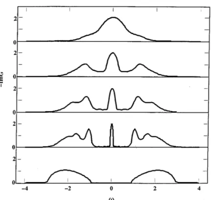
(1996)] (described in the next chapter) emerges as a prominent method to study this model, giving more information of the solution. Figure 1.7 demonstrates the MIT driven by the strong onsite interaction U. As U increases, the bands are split into two bands below and above the Fermi level (lower and upper Hubbard bands), other aspects such as the divergence of the mass enhancement at the transition point [Brinkman and Rice(1970)] are also obtained.

Nevertheless, the Hubbard model is a simple model which neglects important fea-tures of a realistic correlated system. First, the correlated bands are not quite separate from other bands, it may be mixed with other less correlated bands, especially when the interaction is stronger, the correlated bands are split more (to lower and upper Hubbard bands), this mixing becomes more significant. It is therefore necessary to consider the effect of other bands in addition to the correlated ones. Second, there are usually more than one correlated bands (e.g. d orf bands) staying nearly at the same energy level, i.e nearly degenerate, the Hubbard model has to be generalized to take into account more than one correlated band.

Figure1.8summarizes the metals/insulators for various TMOs in perovskite struc-tures. Under the crystal field splitting due to the octahedron MO6, the d bands are split into 3 t2g bands and 2 eg bands staying at higher energy level. Early TMOs,

which consist of light transition metal elements, have partially filledt2g bands at the

Figure 1.7: The evolution of spectral functions for the metal-insulator tran-sition as onsite interaction U increases (from top to bottom panel). From Georges et al. (1996).

to rise to higher energy levels than the p bands, they are in Mott-Hubbard regime. Whereas late TMOs, which has heavier transition metal elements, have filledt2g shell

but partially filled eg shell, the large positive charge of the late transition metal ion

pushes the d bands to lower energy comparable with the p bands, the systems are usually in the charge transfer regime. The magnitude of p-d admixture increases as going from light to heavy transition metal. Understanding how thep-dcovalency (the admixture between p and d bands) affects the electron correlation is an important aspect.

The splitting of the d bands into the 3 t2g and 2 eg nearly degenerate bands

also implies that a multiorbital interaction is required to replace the Hubbard terms

1. Introduction 14

Figure 1.8: The schematic diagram for the metal-insulator transition in TMO perovskite structure ReMO3. The number of d electrons increases from 0 to 8, while the U/W or ∆/W ratio increases by replacing the rare earth Re by elements of smaller atomic radii. From Imada et al. (1998).

the charging energy or the energy cost to add more delectrons, the Hund’s rules are applied such that the electron spin of different orbitals are aligned first followed by the condition of maximal angular momentum. For example, the onsite interaction can have the form

Honsite= U ₋3J 2 ˆ N( ˆN ₋1)₋2JSˆ2₋J 2 ˆ L2. (1.2)

whereJ is the Hund’s coupling representing the Hund’s rules. In multiorbital system, the correlation is not only represented byU but also byJ value [Georges et al.(2013)]. The MIT becomes more complicated with the appearance of the Hund’s coupling, and can occur not only at half-filling but also, for example, at quarter filling (eg systems)

or one-third or two-third filling (t2g systems).

Until recently, there are many advances in understanding the MIT in the Hubbard model. However, there are still many unsolved problems such as how the MIT occurs

in the multiorbital systems or the effect of oxygen bands to this transition. In this thesis, we study the metal-insulator transition in TMOs using dynamical mean-field theory in combination with density functional theory, which have a more complicated multiorbital interaction such as in (1.2), and consider the effect ofp-dcovalency. The study has contribution to the understanding of the MIT and may suggests direction towards more realistic calculations of TMOs.

1.4

Magnetism

Magnetism was discovered a long time ago. The first written evidence comes from the ancient Greece, where Aristotle “reported that Thales of Miletus (625 BC -547 BC) knew lodestone” [du Tr´emolet de Lacheisserie et al. (2005)]. However, until now, it is still a problem of interest in condensed matter physics. Magnetism behaves differently in materials, especially when there is electron correlations, a material may have several types of magnetic phases in its phase diagram. Geometrical frustration can also give complicated magnetic structure, the so-called “frustrated magnetism” may give quantum spin liquid phase or other exotic excitations [Balents (2010)].

There are several basic types of magnetism: ferromagnetism, antiferromagnetism or ferrimagnetism (see Figure1.9). In many TMOs, there are magnetic order patterns different from the usual diamagnetism or paramagnetism. These types of magnetism are very often related to the electron correlation. The rich physics of correlated materials is expressed in their complex phase diagrams such that when a parameter such as the doping level or pressure is changed, the material can change from one type of magnetic order to a different type or to a disordered phase (see Fig. 1.2 for some representative phase diagrams).

Antiferromagnetic order is usually observed in TMOs at low temperature in dif-ferent patterns accompany by a specific orbital order. The pattern of staggered spin

1. Introduction 16

Figure 1.9: Types of magnetic order phases: (A) disordered phase, (B) fer-romagnetism, (C) antiferfer-romagnetism, (D) ferrimagnetism, (E) long periodic magnetic pattern. From Sigma-Aldrich.

and orbital orders is described phenomenologically using Goodenough-Kanamori rules [Goodenough (1958); Kanamori (1959)]. More fruitful discussions about antiferro-magnetism in TMOs can be found inImada et al. (1998) and the references therein. In our study, we focus more on the ferromagnetic order. Ferromagnetism is a straightforward magnetic phase, there is no translation or gauge invariant symmetry breaking, only the spin symmetry is broken. It allows to use the smallest possible unit cell for investigating ferromagnetic order, which simplifies the calculation and separates ferromagnetism from other phases. Ferromagnetism is important in tech-nology such as in spintronics or building memory devices. Ferromagnetism in strongly correlated systems has been studied since the 1930s, however, the correlation effect makes it difficult to solve the problem completely. Therefore, many aspects of ferro-magnetism are not well understood until now.

Ferromagnetism in correlated materials can be divided into two classes. The first class includes materials with localized magnetic moments, usually the rare earth compound with partially filled f shell, which are aligned to form the ferromagnetic order. Because of their localized characteristic, these materials can be mapped to spin systems, in which the most famous one is the Heisenberg model

H=₋X

hiji

JijSiSj. (1.3)

In the other class of materials, which includes transition metal compounds and TMOs, the charge motion is also important, the electrons of conduction bands can carry magnetic moment, it is called “itinerant ferromagnetism”.

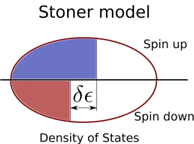
The first attempt to study itinerant ferromagnetism in the theoretical side is from Stoner (1938). By considering the exchange interactionJ between two nearest neighbor sites and the electrons near the Fermi level, he found that when there is

δ difference in energy between spin up and down bands (see Figure 1.10), there is a competition in energy between the cost in kinetic energy and the energy saved from the spin aligned. The increase in kinetic energy is δK _∼ νFδ2 where νF is

the density of states at the Fermi level while the decrease because of spin aligned is _∼ JM2 _{∼ J ν}2

Fδ2 (M is the magnetization). The ferromagnetism is stable if the

change in energy between ferromagnetic and paramagnetic order is negative

δK ₋JM2 =νFδ2−J νF2δ

2 _{<0, (1.4)}

or

J νF >1 (1.5)

Eq. (1.5) is the Stoner’s criteria needed to stabilize ferromagnetism.

1. Introduction 18

Spin up

Spin down

Stoner model

Density of States

Figure 1.10: Stoner model for itinerant ferromagnetism: spin up and down electrons have different occupancy.

reasonable to use a model with correlation to study the magnetic order. Hubbard model (Eq. (1.1)) has been also used for the study of magnetism to understand how correlation drives the magnetic order. A few years after Hubbard proposed his model, Nagaoka proved that if the onsite interaction U is infinitely large, the system with a single hole away from half filling is ferromagnetic with fully spin polarized [Nagaoka (1966)]. However, the conditions for Nagaoka ferromagnetism are extreme, in ther-modynamic limit where the hole density and the U value are finite, it is still unclear about the ferromagnetism [Park et al. (2008)]. At least there exists ferromagnetic order in the Hubbard model if certain conditions are satisfied. Mean field study for the Hubbard model supports Nagaoka’s statement about the ferromagnetism, for ex-ample, Figure 1.11 shows the phase diagram for a two-dimensional Hubbard model in which the ferromagnetic order favors large U values and being doped away from half-filling [Hirsch (1985)].

However, the Hubbard model is a non-trivial model, mean field theory cannot capture the fluctuation around its solution, while perturbation approach may face divergence in the solution with respect to the non-interacting result, especially when

Figure 1.11: The magnetic phase diagram for the Hubbard model from mean field calculation with only nearest neighbor hopping t for the two-dimensional square lattice. The notations are: ρ is the filling, P is paramag-netic order, A is antiferromagparamag-netic order, and F is ferromagparamag-netic order. From Hirsch (1985).

U gets larger. It requires non-perturbative methods to treat the Hubbard model. Until recently, non-perturbative approaches with advances in computational power allow more accurate calculations for the Hubbard model. For one-dimensional Hub-bard model, ferromagnetic order is excluded if there is only nearest neighbor hopping [Lieb and Mattis (1962)], only when extending to longer range electron hopping, fer-romagnetism is allowed under certain circumstances [M¨uller-Hartmann (1995); Daul and Noack (1997)]. In two-dimensional case, it is more difficult with complicated phase diagram. Dynamical mean-field theory (DMFT), the state-of-the-art method for strongly correlated systems, becomes important and gain more insights into the 2D model. DMFT has shown to be able to treat the Hubbard model, capturing the Mott insulating physics [Georges et al. (1996)]. In the topic of magnetism, DMFT shows clearly the antiferromagnetic order exists at half-filling for two-dimensional Hubbard

1. Introduction 20

model [Jarrell et al. (2001); Wang et al. (2009)]. For ferromagnetism, by applying single-site DMFT, Ulmke, Vollhardt et al. showed that the itinerant ferromagnetism in the Hubbard model, beside the U value, depends strongly on the kinetic energy and the lattice structure [Ulmke (1998); Vollhardt et al. (1999)]. It goes far beyond Stoner’s criteria and mean field calculations for the Hubbard model and supports the idea that a density of states peak near the band edge may allow ferromagnetism [Kanamori (1963)].

The Hubbard model, despite being non-trivial, is simple model, far from the re-alistic correlated systems. As mentioned in Section 1.3, extensions for the Hubbard model are the multiorbital models, in which there are more than one degenerate cor-related bands and the interaction is more general with the Hund’s coupling J. The wide range of carrier density (or the filling) and the involvement of the Hund’s cou-pling lead to various behaviors of magnetism. The works on these models, however, are limited, mostly at the extent of model calculations, for example, the theoretical Bethe lattice [Chan et al. (2009); Peters and Pruschke (2010); Peters et al. (2011)]. Similar to the Hubbard model, the magnetism may depend strongly on the lattice structure and the electron hopping in a more general multiorbital model. Therefore, in TMOs, rigorous calculations considering realistic structures are important and can reveal the physics of different lattice structures affect magnetism.

In this thesis, we study the ferromagnetism in early TMOs including the general multiorbital onsite interaction and the realistic lattice structure of materials by using density function theory plus dynamical mean-field theory. We find several conditions under which ferromagnetism may occur and explain why ferromagnetic order occurs in some materials of TMOs but no in others. Our study also considers the ferromag-netism in heterostructures of TMOs and suggests potential designs which can enhance the ferromagnetic order.

1.5

Charged impurity

There is no perfect single crystal for realistic materials. Defects in materials such as dislocation, vacancies or impurities can be found frequently when fabricating a material. There are also impurities staying temporarily inside materials which come from flux of particles used to measure physical properties of materials. These defects and impurities perturb the lattice, modify the lattice constant and change the electronic properties of materials significantly.

Impurity in strongly correlated systems is also an interesting problem [Millis (2003); Alloul et al. (2009)]. A prominent example is the Kondo problem [Hew-son (1997)], where diluted magnetic impurities put into a metallic system and causes a minimum in resistivity as a small value of temperature. It is a “classic” problem of strongly correlated systems and has attracted researchers’ interest for many years. Other impurity problems such as nonmagnetic or charged impurity, lattice defects in correlated systems are also interesting for investigation.

The motivation of our study of charged impurity is to understand how it perturbs the correlated system. When a charge impurity stays on the lattice, it will be screened by electrons (or holes). In a correlated material, the density fluctuation is suppressed, it is interesting to investigate how the screening works. Moreover, charge impurity induces more carrier density in the vicinity, as the density is crucial in strongly corre-lated systems which can increase the charge energy significantly (see (1.2)), it is also important to study how the impurity changes the physics of the neighborhood.

Our work has application in cuprates. Cuprates are TMO compounds which can be high-Tc superconductors. Fig. 1.2B is a schematic phase diagram for cuprates

where superconducting phase can be obtained at low enough temperature and inter-mediate doping. The pseudogap phase exists in the phase diagram of cuprates as a phase where the excitation gap is not well-formed [Damascelli et al. (2003)]. Its physics is believed to give insights to the formation of the Cooper’s pairs is, however,

1. Introduction 22

Figure 1.12: Some patterns of orbital current in the pseudogap phase of cuprates. From Varma(2006).

not fully understood. Varma stated that the pseudogap phase is a time reversal sym-metry breaking phase, in which there is orbital current forming a closed loop that induces local magnetic moment [Varma (1997, 2006)] (see Figure 1.12 for possible patterns of the orbital currents).

There are many attempts from experimentalists to search for this local moment. People mainly use neutron scattering or muon spin relaxation (µSR) to detect this tiny local magnetic field. The results from neutron scattering indeed show that there exists nonzero local moment in the pseudogap phase which vanishes if the material is out of that phase, and thus support Varma’s argument about the orbital current in the pseudogap phase [Fauqu´e et al. (2006); Li et al. (2008); Mook et al. (2008)]. In contrast, it is hardly seen clear evidence for that magnetic moment from µSR measurements [Sonier et al.(2001);MacDougall et al.(2008)], contradicts the results obtained from neutron scattering. Consider the difference between the two methods,

µSR implants a usually positive muon µ+_{, a charged particle into the lattice, while} neutron scattering only uses neutral particles (neutrons) to measure local moment, it is essential to understand how charged particles perturb the lattice in order to explain

the measurements.

Inspired by these experimental work, we study the problem of a charged impurity in strongly correlated systems. Our work using dynamical mean-field theory method gives some insights to this interesting controversy and also to the understanding of the feedback from the lattice to theµSR measurements. Our study shows that dynamical mean-field theory can be a useful method to study impurities and defects in correlated materials.

2. Formalism 24

Chapter 2

Formalism

2.1

General description

In most of the cases that we study, materials are in perovskite formRMO3, where each transition metal M is surrounded by 6 oxygens. The octahedron MO6 decides the electronic structure of the system. The physics is controlled by the charge transfer between the oxygen and transition metal ions and by the strong electronic correlation on the transition metal sites. On the other hand, lattice structure is different for different materials. The octahedra MO6 are not usually aligned, they can be tilted or rotated depending on specific material. The rotations and tilts can act to lift the degeneracy of the transition metal d levels and to change the bandwidth. It is important to understand the connection between lattice structure and the correlation and how they affect the physics.

In this section, we will give an overview of the electronic structure of TMOs, which range of energy to be considered and how it might be changed when there is strong electron correlation. We also introduce possible realistic structure of TMOs in the perovskite form and a general way to describe the structure in the calculations.