A New Risk Factor based on Equity Duration

This Online-Appendix presents additional empirical analyses to support the robustness of our main results. It contains four subsections.

In the first subsection, we vary some assumptions regarding the calculation of our dura-tion measure. In total, we consider seven possible variadura-tions of our original configuradura-tion. We present summary statistics, excess returns, and alphas of duration long-short-portfolios for all seven specifications in Table 1.

In the second subsection, we rerun our analyses from Sections 3.3 and 3.4 of the main paper for different subsamples and use value-weighted instead of equally-weighted returns. These analyses imply portfolio sorts and factor spanning tests. Since we find no significant excess return for value-weighted portfolios in Table 2, we exclude the smallest 20% of stocks and sort based on equally-weighted returns in Table 3. We find significant excess returns comparable to our original results, so we can rule out that these are merely driven by small/microcap stocks. Instead, we find that there is no duration effect for the largest stocks in our sample, possibly due to better hedging options against reinvestment risk, broader diversification, and higher accessibility to diverse financing sources for very large firms. After excluding the smallest and largest 20% of stocks from our sample, we also find significant excess returns and alphas for value-weighted long-short duration portfolios in Table 4. We find further support for our conjecture that firm size may mitigate the effects of reinvestment risk by performing double-sorts on size and duration for equally- and value-weighted portfolios in Table 5. As a further robustness test, we exclude technology firms from our sample in Table 6. Technology firms are identified using the SIC code classification proposed by Villalonga and Amit (2006). Finally, Table 7 reports results on factor spanning tests using a value-weighted construction of LDMHD. Previous results remain qualitatively unchanged, even though significance levels vary compared to our main analysis.

The third subsection provides summary statistics and correlation coefficients for our LDMHDmeasure as well as MKT,SMB,HML, and the state variables we use (see Table 8). The correlation coefficients support the variable interactions also detected in the factor spanning tests in the main part of the paper.

Subsection 4 provides several analyses using different specifications of our asset pricing tests. Recall that in the base case, we run Fama-MacBeth-regressions on LDMHD, and the factors MKT, HML, and SMB from the Fama-French-3-factor model, and state variable innovations

[

_DIV, RFc, TERM

\

, and DEF

[

. For all specifications tested in this section, the coefficient on LDMHDremains positive and both economically and statistically significant. For Tables 9 and 10, we do not take the difference between below-median and above-median equity duration as LDMHDreturn spread, but instead use the difference between the two most extreme duration portfolios P1 and P10. Noticeably, this altered version of LDMHD carries a higher premium and a higher price of risk (and remains highly significant) while all other effects remain similar in size and significance. In Table 11, we include all five Factors from Fama and French (2015), plus momentum, in the analysis. In the model for Table 12, we exclude the intercept from our regressions to test if our model is correctly specified. We find a similar estimate for the market price of duration risk with and without an intercept, which indicates that our model is specified correctly as the intercept should be zero theoretically. For Table 13, state variable innovations are estimated based on a simple AR(1) process instead of the VAR system we use in our main model, while we employ ordinary least squares (OLS) instead of GLS regressions in Table 14. Both of these robustness tests serve the purpose to avoid overfitting of our model. In particular, if the number of portfolios is relatively large compared to the number of analyzed months, the estimate for the portfolio return covariance matrix required by the GLS approach may be inaccurate (Lewellen et al., 2010). In Table 15, we split our sample period into two subperiods of equal size to determine whether our results are driven by a specific time period, which does not appear to be the case. For Tables 16 to 22, we vary several assumptions regarding the construction of our test portfolios and asset pricing factors. This includes several value-weighted portfolios, differentLDMHD weighting schemes, and different numbers of portfolios as test assets. Again, all results with respect to our LDMHDfactor remain robust.

1.

D

ifferent

S

pecifications for

E

quity

D

uration

C

alculation

Table 1. Different Methodologies for the Calculation of Equity Duration

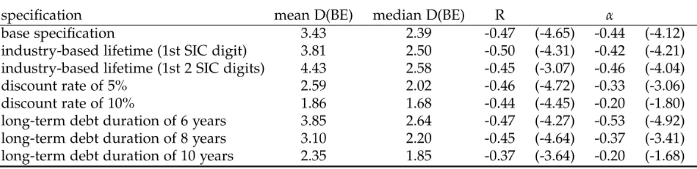
This table presents robustness tests with respect to different calculation methods for equity duration. The standard duration calculation method uses the overall sample median of gross PPE divided by annual depreciation for the lifetime of long-term tangible assets (instead of industry-specific values), a zero discount rate in the duration calculation of long-term tangible and intangible assets, and a duration of 7.12 years for the long-term debt exceeding a maturity of five years. The robustness checks alter these assumptions. The first column states the changed specification, the second and third column the corresponding mean and median book equity duration. The remaining columns refer to the average monthly long-short-return between the extreme duration deciles equivalent to Table 3 in the main paper. Both unadjusted subsequent returns R and Fama-French-5-factor-plus-momentum-adjusted returnsαare provided. The sample period covers July 1970 to December 2016.

Alphas and returns are stated in %. The t-statistics in parentheses are based on standard errors following Newey and West (1987).

specification mean D(BE) median D(BE) R α

base specification 3.43 2.39 -0.47 (-4.65) -0.44 (-4.12)

industry-based lifetime (1st SIC digit) 3.81 2.50 -0.50 (-4.31) -0.42 (-4.21) industry-based lifetime (1st 2 SIC digits) 4.43 2.58 -0.45 (-3.07) -0.46 (-4.04)

discount rate of 5% 2.59 2.02 -0.46 (-4.72) -0.33 (-3.06)

discount rate of 10% 1.86 1.68 -0.44 (-4.45) -0.20 (-1.80)

long-term debt duration of 6 years 3.85 2.64 -0.47 (-4.27) -0.53 (-4.92) long-term debt duration of 8 years 3.10 2.20 -0.45 (-4.64) -0.37 (-3.41) long-term debt duration of 10 years 2.35 1.85 -0.37 (-3.64) -0.20 (-1.68)

2.

V

arious

P

ortfolio

R

eturn

C

alculation

M

ethods

Table 2. Portfolio Sorts based on Equity Duration – Value-Weighted

This table reports the value-weighted returns of decile portfolios for the subsequent months. Each month, stocks are allocated to one of the ten portfolios based on book equity duration deciles. The table reports both unadjusted subsequent returns R and portfolio alphas and factor loadings with respect to the Fama-French-5-factor-plus-momentum-model. The last column reports each portfolio’s value-weighted average book equity duration. The sample period covers July 1970 to December 2016. Alphas and returns are stated in %. The t-statistics in parentheses refer to the difference between the extreme decile portfolios and are based on standard errors following Newey and West (1987).

D(BE) R α βMKT βSMB βHML βRMW βCMA βWML D(BE)

low 1.12 -0.01 1.08 0.33 -0.08 0.13 0.29 -0.08 -2.26 2 1.15 0.16 1.03 0.18 -0.07 0.01 0.03 -0.02 0.48 3 1.06 0.05 1.03 0.17 -0.17 -0.02 0.18 -0.00 1.16 4 0.97 0.05 0.98 0.18 -0.23 -0.15 0.07 0.04 1.70 5 1.00 0.12 1.03 0.15 -0.20 -0.21 0.05 -0.02 2.24 6 1.00 0.15 0.96 0.01 -0.23 -0.16 -0.01 0.04 2.88 7 1.04 0.20 0.95 -0.16 -0.10 0.06 0.01 -0.06 3.70 8 0.97 -0.00 0.96 -0.13 -0.13 0.23 0.10 0.01 4.76 9 1.02 0.03 0.94 -0.05 -0.03 0.17 0.06 0.02 6.49 high 1.04 -0.01 1.01 0.15 -0.07 0.21 0.02 0.00 11.21 10-1 -0.08 0.00 -0.08 -0.19 0.01 0.08 -0.27 0.08 13.46 t(10-1) (-0.61) (0.05) (-1.97) (-2.96) (0.11) (0.92) (-2.42) (1.79) (29.67)

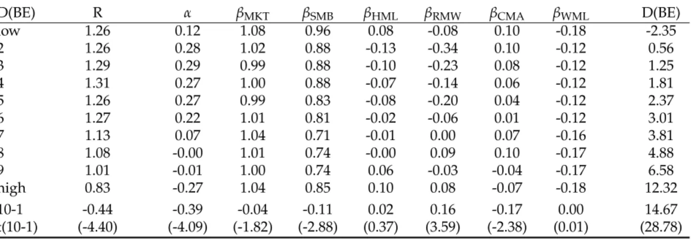
Table 3. Portfolio Sorts based on Equity Duration – Excluding Small Stocks

This table reports the equally-weighted returns of decile portfolios for the subsequent months. Each month, stocks are allocated to one of the ten portfolios based on book equity duration deciles. The table reports both unadjusted subsequent returns R and portfolio alphas and factor loadings with respect to the Fama-French-5-factor-plus-momentum-model. The last column reports each portfolio’s average book equity duration. For each month, small stocks that are below the 20%-size-quantile are excluded from the sample. The sample period covers July 1970 to December 2016. Alphas and returns are stated in %. The t-statistics in parentheses refer to the difference between the extreme decile portfolios and are based on standard errors following Newey and West (1987).

D(BE) R α βMKT βSMB βHML βRMW βCMA βWML D(BE)

low 1.26 0.12 1.08 0.96 0.08 -0.08 0.10 -0.18 -2.35 2 1.26 0.28 1.02 0.88 -0.13 -0.34 0.10 -0.12 0.56 3 1.29 0.29 0.99 0.88 -0.10 -0.23 0.08 -0.12 1.25 4 1.31 0.27 1.00 0.88 -0.07 -0.14 0.06 -0.12 1.81 5 1.26 0.27 0.99 0.83 -0.08 -0.20 0.04 -0.12 2.37 6 1.27 0.22 1.01 0.81 -0.02 -0.06 0.01 -0.12 3.01 7 1.13 0.07 1.04 0.71 -0.01 0.00 0.07 -0.16 3.81

Table 4. Portfolio Sorts based on Equity Duration – Excluding Small Stocks and Large Stocks

This table reports the value-weighted returns of decile portfolios for the subsequent months. Each month, stocks are allocated to one of the ten portfolios based on book equity duration deciles. The table reports both unadjusted subsequent returns R and portfolio alphas and factor loadings with respect to the Fama-French-5-factor-plus-momentum-model. The last column reports each portfolio’s value-weighted average book equity duration. For each month, small stocks that are below the 20%-size-quantile and large stocks that are above the 80%-size-quantile are excluded from the sample. The sample period covers July 1970 to December 2016. Alphas and returns are stated in %. The t-statistics in parentheses refer to the difference between the extreme decile portfolios and

are based on standard errors following Newey and West (1987).

D(BE) R α βMKT βSMB βHML βRMW βCMA βWML D(BE)

low 1.21 0.05 1.13 0.98 0.04 -0.04 0.04 -0.17 -2.71 2 1.26 0.26 1.03 0.90 -0.18 -0.35 0.10 -0.07 0.44 3 1.20 0.18 1.02 0.93 -0.10 -0.28 0.02 -0.08 1.12 4 1.29 0.27 1.02 0.90 -0.13 -0.15 -0.00 -0.10 1.65 5 1.27 0.20 1.02 0.92 -0.10 -0.15 0.04 -0.07 2.19 6 1.32 0.21 1.03 0.87 -0.03 -0.01 0.05 -0.11 2.80 7 1.17 0.05 1.08 0.87 -0.04 0.07 0.04 -0.15 3.56 8 1.16 -0.02 1.08 0.87 0.03 0.17 0.05 -0.16 4.62 9 1.11 0.00 1.04 0.85 0.04 0.05 0.01 -0.16 6.32 high 0.87 -0.31 1.10 0.90 0.14 0.16 -0.17 -0.13 12.08 10-1 -0.34 -0.36 -0.03 -0.08 0.10 0.20 -0.20 0.04 14.79 t(10-1) (-3.09) (-3.47) (-1.01) (-1.62) (1.77) (2.91) (-2.25) (1.09) (31.07) 5

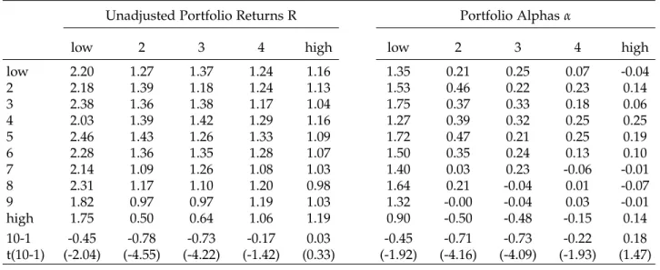
Table 5. Conditional Double Sorts on Size and Equity Duration

This table reports the equally-weighted (Panel A) and value-weighted (Panel B) returns of cross-sectional conditional double sorts. First, each stock is allocated to one quintile based on its market capitalization. Second, within each quintile, every stock is assigned to one decile based on its book equity duration D(BE). This table presents both unadjusted subsequent returns R and portfolio alphasαwith respect to the Fama-French-5-factor-plus-momentum-model. The sample period covers

July 1970 to December 2016. Alphas and returns are stated in %. The t-statistics in parentheses refer to the difference between the extreme decile portfolios and are based on standard errors following Newey and West (1987).

Panel A: Equally-Weighted Returns

Unadjusted Portfolio Returns R Portfolio Alphasα

low 2 3 4 high low 2 3 4 high

low 2.20 1.27 1.37 1.24 1.16 1.35 0.21 0.25 0.07 -0.04 2 2.18 1.39 1.18 1.24 1.13 1.53 0.46 0.22 0.23 0.14 3 2.38 1.36 1.38 1.17 1.04 1.75 0.37 0.33 0.18 0.06 4 2.03 1.39 1.42 1.29 1.16 1.27 0.39 0.32 0.25 0.25 5 2.46 1.43 1.26 1.33 1.09 1.72 0.47 0.21 0.25 0.19 6 2.28 1.36 1.35 1.28 1.07 1.50 0.35 0.24 0.13 0.10 7 2.14 1.09 1.26 1.08 1.03 1.40 0.03 0.23 -0.06 -0.01 8 2.31 1.17 1.10 1.20 0.98 1.64 0.21 -0.04 0.01 -0.07 9 1.82 0.97 0.97 1.19 1.03 1.32 -0.00 -0.04 0.03 -0.01 high 1.75 0.50 0.64 1.06 1.19 0.90 -0.50 -0.48 -0.15 0.14 10-1 -0.45 -0.78 -0.73 -0.17 0.03 -0.45 -0.71 -0.73 -0.22 0.18 t(10-1) (-2.04) (-4.55) (-4.22) (-1.42) (0.33) (-1.92) (-4.16) (-4.09) (-1.93) (1.47)

Panel B: Value-Weighted Returns

Unadjusted Portfolio Returns R Portfolio Alphasα

low 2 3 4 high low 2 3 4 high

low 1.81 1.27 1.37 1.19 1.08 0.93 0.18 0.23 0.01 0.03 2 1.69 1.38 1.23 1.21 1.07 1.00 0.44 0.31 0.19 0.03 3 1.74 1.38 1.37 1.15 0.91 1.05 0.37 0.32 0.17 -0.00 4 1.67 1.31 1.40 1.28 1.06 0.81 0.27 0.31 0.24 0.20 5 1.97 1.38 1.21 1.29 1.03 1.18 0.42 0.15 0.23 0.25 6 1.71 1.34 1.33 1.27 0.91 0.92 0.31 0.24 0.14 0.13 7 1.72 1.14 1.22 1.10 1.03 0.93 0.10 0.17 -0.02 0.14 8 1.63 1.13 1.10 1.21 0.97 0.84 0.16 -0.04 0.02 0.02 9 1.05 0.95 1.01 1.19 0.92 0.35 -0.04 0.00 0.02 -0.05 high 1.13 0.46 0.67 1.08 1.12 0.26 -0.57 -0.42 -0.14 0.13 10-1 -0.68 -0.81 -0.69 -0.10 0.04 -0.67 -0.75 -0.65 -0.14 0.10 t(10-1) (-2.91) (-4.51) (-4.16) (-0.84) (0.28) (-2.65) (-4.22) (-3.71) (-1.23) (0.69)

Table 6. Portfolio Sorts based on Equity Duration – Without Technology Firms

This table reports the equally-weighted returns of decile portfolios for the subsequent months. Each month, stocks are allocated to one of the ten portfolios based on book equity duration. The table reports unadjusted subsequent returns R, portfolio alphasα, and factor loadings with respect to

the Fama-French-5-factor-plus-momentum-model. The last column reports each portfolio’s average book equity duration. The sample does not include technology firms (33.72% of the original firm-month-observations), that is, firms with SIC codes 35, 36, 38, or 73. The sample period covers July 1970 to December 2016. Alphas and returns are stated in %. The t-statistics in parentheses refer to the difference between the extreme decile portfolios and are based on standard errors following Newey and West (1987).

R α βMKT βSMB βHML βRMW βCMA βWML D(BE) low 1.36 0.17 1.02 0.97 0.19 0.08 0.18 -0.22 -2.83 2 1.45 0.43 0.91 0.87 0.00 -0.12 0.16 -0.16 0.40 3 1.36 0.28 0.92 0.90 0.03 -0.03 0.21 -0.16 1.13 4 1.42 0.31 0.93 0.88 0.09 0.05 0.12 -0.15 1.72 5 1.33 0.18 0.94 0.83 0.09 0.11 0.20 -0.14 2.33 6 1.36 0.20 0.95 0.77 0.17 0.17 0.08 -0.15 3.00 7 1.25 0.14 0.97 0.73 0.16 0.15 0.05 -0.18 3.84 8 1.23 0.15 0.95 0.75 0.18 0.11 0.00 -0.18 4.97 9 1.07 0.06 0.95 0.80 0.19 0.05 -0.06 -0.25 6.83 high 0.95 -0.16 1.00 0.91 0.14 0.09 -0.01 -0.22 13.27 10-1 -0.42 -0.33 -0.01 -0.05 -0.05 0.02 -0.18 0.01 16.10 t(10-1) (-3.39) (-2.28) (-0.45) (-1.18) (-0.78) (0.25) (-1.73) (0.16) (30.58) 7

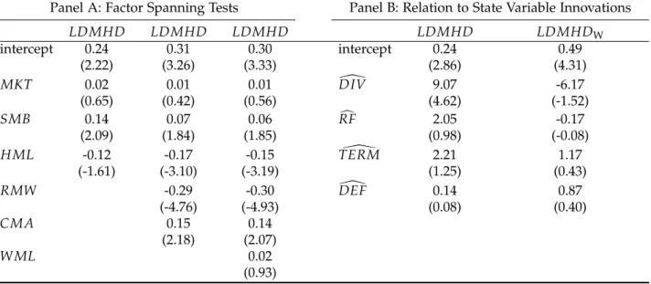
Table 7. Interaction of LDMHD with Risk Factors and State Variable Innovations

This table reports time series regression estimates based on monthly data. The factor spanning tests in Panel A useLDMHDas dependent variable and the Fama-French-5-factor-plus-momentum-factors as explanatory variables. In Panel B, the dependent variables are LDMHDandLDMHDW. In contrast to the base scenario,LDMHDis based on value-weighted returns. For each month, small stocks that are below the 20%-size-quantile and large stocks that are above the 80%-size-quantile are excluded from the factor construction. LDMHDWis the equally-weighted return spread between firms with below-median equity duration and above-median equity duration as introduced by Weber (2018). The explanatory variables are the innovations in the market dividend yieldDIV, the risk-free rate RF, the term spreadTERM, and the default spreadDEF. Innovations are estimated based on a vector-autoregressive model. The sample period covers July 1970 to December 2016; for the analysis includingLDMHDW, the sample period ends in June 2014. The intercept estimates are in %. The t-statistics in parentheses are based on standard errors following Newey and West (1987).

Panel A: Factor Spanning Tests Panel B: Relation to State Variable Innovations

LDMHD LDMHD LDMHD LDMHD LDMHDW intercept 0.24 0.31 0.30 intercept 0.24 0.49 (2.22) (3.26) (3.33) (2.86) (4.31) MKT 0.02 0.01 0.01 [_{DIV 9.07 -6.17} (0.65) (0.42) (0.56) (4.62) (-1.52) SMB 0.14 0.07 0.06 RFc 2.05 -0.17 (2.09) (1.84) (1.85) (0.98) (-0.08) HML -0.12 -0.17 -0.15 _TERM\ _{2.21 1.17} (-1.61) (-3.10) (-3.19) (1.25) (0.43) RMW -0.29 -0.30 _DEF[ _{0.14 0.87} (-4.76) (-4.93) (0.08) (0.40) CMA 0.15 0.14 (2.18) (2.07) W ML 0.02 (0.93)

3.

S

ummary

S

tatistics for the

D

ifferent

F

actors

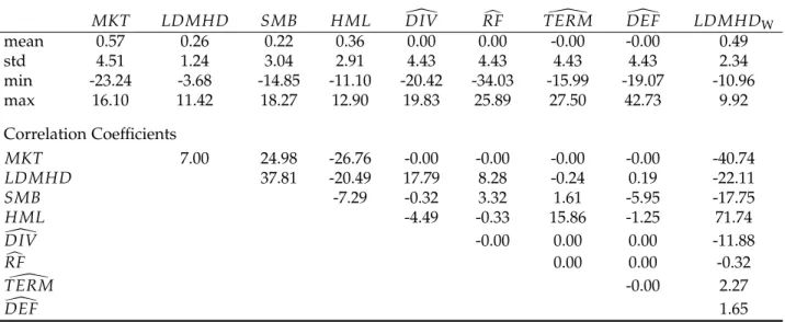
Table 8. Summary Statistics and Correlation Coefficients

This table reports mean, standard deviation, minimum, and maximum of various time series. Moreover, correlation coefficients are provided. The time series are the excess market returnMKT, the duration factor LDMHD, the size factorSMB, the value factorHML, and the innovations in the market dividend yield DIV, the risk-free rate RF, the term spread TERM, and the default spreadDEF. LDMHDW is the return spread between firms with below-median equity duration and above-median equity duration as introduced by Weber (2018). The sample period covers July 1970 to December 2016; for the analyses includingLDMHDW, the sample period ends in June 2014. The factor returns are in %.

MKT LDMHD SMB HML _DIV[ RFc TERM\ DEF[ LDMHDW

mean 0.57 0.26 0.22 0.36 0.00 0.00 -0.00 -0.00 0.49 std 4.51 1.24 3.04 2.91 4.43 4.43 4.43 4.43 2.34 min -23.24 -3.68 -14.85 -11.10 -20.42 -34.03 -15.99 -19.07 -10.96 max 16.10 11.42 18.27 12.90 19.83 25.89 27.50 42.73 9.92 Correlation Coefficients MKT 7.00 24.98 -26.76 -0.00 -0.00 -0.00 -0.00 -40.74 LDMHD 37.81 -20.49 17.79 8.28 -0.24 0.19 -22.11 SMB -7.29 -0.32 3.32 1.61 -5.95 -17.75 HML -4.49 -0.33 15.86 -1.25 71.74 [ DIV -0.00 0.00 0.00 -11.88 c RF 0.00 0.00 -0.32 \ TERM -0.00 2.27 [ DEF 1.65 9

4.

D

ifferent

S

pecifications of

A

sset

P

ricing

T

ests

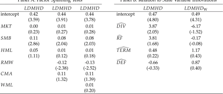
Table 9. Interaction of LDMHD with Risk Factors and State Variable Innovations – LDMHD Based on Extreme Deciles

This table reports time series regression estimates based on monthly data. The factor spanning tests in Panel A useLDMHDas dependent variable and the Fama-French-5-factor-plus-momentum-factors as explanatory variables. In Panel B, the dependent variables are LDMHDandLDMHDW.

LDMHDWis the return spread between firms with below-median equity duration and above-median equity duration as introduced by Weber (2018). The explanatory variables are the innovations in the market dividend yield DIV, the risk-free rateRF, the term spread TERM, and the default spread

DEF. Innovations are estimated based on a vector-autoregressive model. The sample period covers July 1970 to December 2016; for the analysis including LDMHDW, the sample period ends in June 2014. Intercept estimates are stated in %. The t-statistics in parentheses are based on standard errors following Newey and West (1987).

Panel A: Factor Spanning Tests Panel B: Relation to State Variable Innovations

LDMHD LDMHD LDMHD LDMHD LDMHDW intercept 0.42 0.44 0.44 intercept 0.47 0.49 (3.59) (3.91) (3.78) (4.80) (4.31) MKT 0.00 0.01 0.01 [_{DIV 3.87 -6.17} (0.23) (0.27) (0.28) (2.05) (-1.52) SMB 0.11 0.08 0.08 RFc 3.81 -0.17 (2.86) (2.04) (2.03) (1.68) (-0.08) HML 0.05 0.01 0.01 _TERM\ _{0.48 1.17} (1.11) (0.12) (0.18) (0.22) (0.43) RMW -0.12 -0.13 _DEF[ _{-0.66 0.87} (-2.38) (-2.52) (-0.33) (0.40) CMA 0.11 0.11 (1.32) (1.39) W ML 0.01 (0.20)

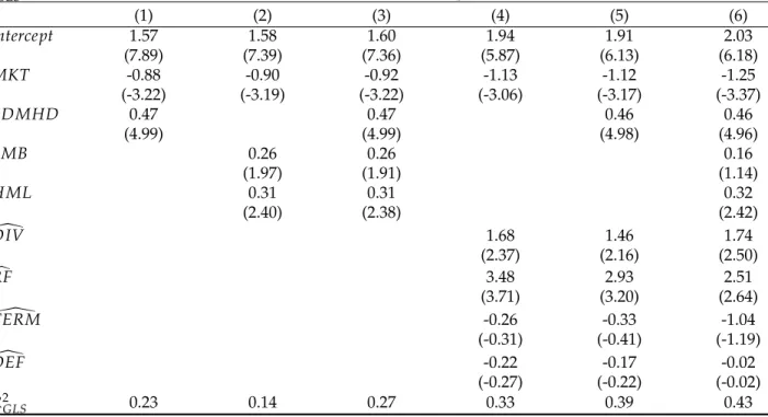
Table 10. Prices of Risk – LDMHD Based on Extreme Deciles

This table presents the prices of risk for different risk factors using Fama-MacBeth-regressions. 25 equally-weighted size/book-to-market portfolios and 10 equally-weighted portfolios based on book equity duration serve as the 35 test assets. The risk factors are the excess market return MKT, the duration factorLDMHD, the size factorSMB, the value factorHML, and the innovations in the market dividend yieldDIV, the risk-free rateRF, the term spreadTERM, and the default spread

DEF. The sample period is July 1970 to December 2016. The corresponding GLS-estimates are stated in %. The t-statistics in parentheses are based on standard errors following Shanken (1992). The

R2

GLS is calculated in accordance with Kandel and Stambaugh (1995).

(1) (2) (3) (4) (5) (6) intercept 1.57 1.58 1.60 1.94 1.91 2.03 (7.89) (7.39) (7.36) (5.87) (6.13) (6.18) MKT -0.88 -0.90 -0.92 -1.13 -1.12 -1.25 (-3.22) (-3.19) (-3.22) (-3.06) (-3.17) (-3.37) LDMHD 0.47 0.47 0.46 0.46 (4.99) (4.99) (4.98) (4.96) SMB 0.26 0.26 0.16 (1.97) (1.91) (1.14) HML 0.31 0.31 0.32 (2.40) (2.38) (2.42) [ DIV 1.68 1.46 1.74 (2.37) (2.16) (2.50) c RF 3.48 2.93 2.51 (3.71) (3.20) (2.64) \ TERM -0.26 -0.33 -1.04 (-0.31) (-0.41) (-1.19) [ DEF -0.22 -0.17 -0.02 (-0.27) (-0.22) (-0.02) R2_GLS 0.23 0.14 0.27 0.33 0.39 0.43 11

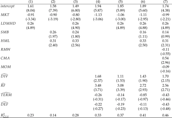
Table 11. Prices of Risk – Considering Additional Risk Factors

This table presents the prices of risk for different risk factors using Fama-MacBeth-regressions. 25 equally-weighted size/book-to-market portfolios and ten equally-weighted portfolios based on book equity duration serve as the 35 test assets. The risk factors are the excess market return MKT, the duration factor LDMHD, the size factorSMB, the value factor HML, the profitability factor

RMW, the investment factorCMA, the momentum factorW ML, and the innovations in the market dividend yieldDIV, the risk-free rateRF, the term spreadTERM, and the default spreadDEF. The sample period is July 1970 to December 2016. The corresponding GLS-estimates are stated in %. The t-statistics in parentheses are based on standard errors following Shanken (1992). TheR2

GLS is

calculated in accordance with Kandel and Stambaugh (1995).

(1) (2) (3) (4) (5) (6) (7) intercept 1.61 1.58 1.49 1.94 1.85 1.89 1.74 (8.04) (7.39) (6.80) (5.87) (5.89) (5.60) (4.38) MKT -0.91 -0.90 -0.80 -1.13 -1.06 -1.11 -0.99 (-3.34) (-3.19) (-2.80) (-3.06) (-3.00) (-2.95) (-2.21) LDMHD 0.26 0.26 0.26 0.26 0.26 (4.89) (4.90) (4.89) (4.88) (4.89) SMB 0.26 0.24 0.16 0.14 (1.97) (1.80) (1.11) (0.99) HML 0.31 0.33 0.33 0.31 (2.40) (2.56) (2.50) (2.31) RMW -0.11 (-0.55) CMA 0.54 (2.96) MOM -0.09 (-0.16) [ DIV 1.68 1.11 1.43 1.70 (2.37) (1.53) (1.90) (2.15) c RF 3.48 3.08 2.72 2.56 (3.71) (3.39) (2.93) (2.71) \ TERM -0.26 -0.14 -0.85 -0.43 (-0.31) (-0.17) (-0.97) (-0.46) [ DEF -0.22 -0.19 -0.11 -0.43 (-0.27) (-0.23) (-0.13) (-0.48) R2_GLS 0.23 0.14 0.28 0.33 0.37 0.41 0.46

Table 12. Prices of Risk – Estimation Without Intercept

This table presents the prices of risk for different risk factors using Fama-MacBeth-regressions. 25 equally-weighted size/book-to-market portfolios and ten equally-weighted portfolios based on book equity duration serve as the 35 test assets. The risk factors are the excess market return MKT, the duration factorLDMHD, the size factorSMB, the value factorHML, and the innovations in the market dividend yieldDIV, the risk-free rateRF, the term spreadTERM, and the default spread

DEF. In contrast to the base scenario, the intercept is set to zero in all regressions. The sample period is July 1970 to December 2016. The corresponding GLS-estimates are stated in %. The t-statistics in parentheses are based on standard errors following Shanken (1992). Note that theR2

GLSfollowing

Kandel and Stambaugh (1995) is not applicable if the intercept is forced to zero.

(1) (2) (3) (4) (5) (6) MKT 0.62 0.62 0.62 0.69 0.67 0.68 (3.21) (3.16) (3.20) (3.48) (3.36) (3.43) LDMHD 0.26 0.26 0.26 0.26 (4.88) (4.87) (4.88) (4.87) SMB 0.29 0.27 0.19 (2.19) (1.98) (1.34) HML 0.40 0.41 0.42 (3.06) (3.20) (3.12) [ DIV -0.17 -0.85 -0.61 (-0.25) (-1.20) (-0.88) c RF 3.82 3.22 3.16 (3.81) (3.24) (3.23) \ TERM 2.54 2.54 1.95 (3.42) (3.53) (2.55) [ DEF 0.46 0.47 0.21 (0.52) (0.55) (0.24) 13

Table 13. Prices of Risk – State Variable Innovations Based on AR(1) processes

This table presents the prices of risk for different risk factors using Fama-MacBeth-regressions. 25 equally-weighted size/book-to-market portfolios and ten equally-weighted portfolios based on book equity duration serve as the 35 test assets. The risk factors are the excess market return MKT, the duration factor LDMHD, the size factorSMB, the value factorHML, and the innovations in the market dividend yield DIV, the risk-free rate RF, the term spread TERM, and the default spread DEF. In contrast to the base scenario, the state variable innovations are calculated based on AR(1) processes instead of a VAR system. The sample period is July 1970 to December 2016. The corresponding GLS-estimates are stated in %. The t-statistics in parentheses are based on standard errors following Shanken (1992). Note that the R2_GLS following Kandel and Stambaugh (1995) is not applicable if the intercept is forced to zero.

(1) (2) (3) (4) (5) (6) intercept 1.61 1.58 1.49 1.85 1.73 1.70 (8.04) (7.39) (6.80) (6.29) (6.27) (5.51) MKT -0.91 -0.90 -0.80 -1.04 -0.96 -0.94 (-3.34) (-3.19) (-2.80) (-3.08) (-2.96) (-2.66) LDMHD 0.26 0.26 0.26 0.26 (4.89) (4.90) (4.87) (4.86) SMB 0.26 0.24 0.18 (1.97) (1.80) (1.31) HML 0.31 0.33 0.34 (2.40) (2.56) (2.55) [ DIV 1.38 0.66 0.95 (2.04) (0.95) (1.29) c RF 3.02 2.49 2.29 (3.34) (2.88) (2.54) \ TERM -0.70 -0.38 -1.06 (-0.85) (-0.49) (-1.20) [ DEF -1.14 -0.90 -0.86 (-1.52) (-1.29) (-1.21) R2 GLS 0.23 0.14 0.28 0.28 0.34 0.38

Table 14. Prices of Risk – Use of OLS instead of GLS

This table presents the prices of risk for different risk factors using Fama-MacBeth-regressions. 25 equally-weighted size/book-to-market portfolios and ten equally-weighted portfolios based on book equity duration serve as the 35 test assets. The risk factors are the excess market return MKT, the duration factorLDMHD, the size factorSMB, the value factorHML, and the innovations in the market dividend yieldDIV, the risk-free rateRF, the term spreadTERM, and the default spread

DEF. The sample period is July 1970 to December 2016. The corresponding OLS-estimates are stated in %. The t-statistics in parentheses are based on standard errors following Shanken (1992). The

R2

OLSis calculated in accordance with Jagannathan and Wang (1993).

(1) (2) (3) (4) (5) (6) intercept 2.36 1.62 1.44 1.85 1.76 2.14 (6.74) (5.85) (5.13) (3.63) (3.72) (5.44) MKT -1.44 -0.93 -0.70 -0.98 -0.93 -1.33 (-4.06) (-2.81) (-2.11) (-1.84) (-1.87) (-3.14) LDMHD 0.22 0.26 0.21 0.30 (2.23) (3.99) (2.73) (5.20) SMB 0.22 0.14 0.14 (1.48) (0.96) (0.99) HML 0.36 0.40 0.39 (2.72) (3.00) (2.87) [ DIV 0.84 -0.08 1.85 (0.67) (-0.07) (2.02) c RF 5.04 3.49 1.57 (2.90) (2.58) (1.36) \ TERM 2.58 2.79 -1.54 (1.40) (1.69) (-1.48) [ DEF 0.74 1.77 1.29 (0.39) (1.21) (1.04) R2_OLS 0.52 0.57 0.71 0.65 0.68 0.76 15

Table 15. Prices of Risk – Subperiod Analysis

This table presents the prices of risk for different risk factors using Fama-MacBeth-regressions. 25 equally-weighted size/book-to-market portfolios and ten equally-weighted portfolios based on book equity duration serve as the 35 test assets. The risk factors are the excess market return MKT, the duration factor LDMHD, the size factorSMB, the value factor HML, and the innovations in the market dividend yield DIV, the risk-free rateRF, the term spread TERM, and the default spread

DEF. The sample period is July 1970 to September 1993 in Panel A and October 1993 to December 2016 in Panel B. The corresponding GLS-estimates are stated in %. The t-statistics in parentheses are based on standard errors following Shanken (1992). The R2

GLS is calculated in accordance with

Kandel and Stambaugh (1995).

Panel A (1) (2) (3) (4) (5) (6) intercept 1.10 0.99 0.94 0.86 0.83 0.82 (4.40) (3.53) (3.30) (2.88) (2.73) (2.57) MKT -0.50 -0.40 -0.35 -0.26 -0.22 -0.22 (-1.35) (-1.02) (-0.88) (-0.64) (-0.55) (-0.52) LDMHD 0.28 0.28 0.28 0.28 (4.38) (4.37) (4.34) (4.35) SMB 0.22 0.22 0.22 (1.25) (1.20) (1.20) HML 0.48 0.47 0.47 (2.81) (2.78) (2.73) [ DIV 0.38 -0.05 -0.03 (0.58) (-0.07) (-0.04) c RF 2.19 1.80 1.75 (2.13) (1.74) (1.63) \ TERM 1.42 1.60 1.54 (1.92) (2.15) (1.89) [ DEF 0.97 0.82 0.85 (1.09) (0.92) (0.90) R2_GLS 0.31 0.15 0.35 0.19 0.44 0.44 Panel B (1) (2) (3) (4) (5) (6) intercept 1.34 1.32 1.30 0.97 1.02 0.90 (5.77) (5.55) (5.37) (3.07) (3.37) (2.53) MKT -0.68 -0.67 -0.65 -0.33 -0.40 -0.28 (-1.93) (-1.89) (-1.83) (-0.82) (-1.00) (-0.63) LDMHD 0.23 0.23 0.23 0.23 (2.79) (2.79) (2.77) (2.78) SMB 0.41 0.39 0.30 (2.10) (1.99) (1.47) HML 0.12 0.15 0.29 (0.61) (0.78) (1.41) [ DIV -0.50 -0.70 -0.16 (-1.15) (-1.58) (-0.30)

Table 16. Prices of Risk – LDMHD based on Terciles

This table presents the prices of risk for different risk factors using Fama-MacBeth-regressions. 25 equally-weighted size/book-to-market portfolios and ten equally-weighted portfolios based on book equity duration serve as the 35 test assets. The risk factors are the excess market return MKT, the duration factorLDMHD, the size factorSMB, the value factorHML, and the innovations in the market dividend yieldDIV, the risk-free rateRF, the term spreadTERM, and the default spread

DEF. In contrast to the base scenario,LDMHDis calculated based on the return difference between low- and high duration tercile portfolios. The sample period is July 1970 to December 2016. The corresponding GLS-estimates are stated in %. The t-statistics in parentheses are based on standard errors following Shanken (1992). TheR2_GLSis calculated in accordance with Kandel and Stambaugh (1995). (1) (2) (3) (4) (5) (6) intercept 1.61 1.58 1.51 1.94 1.85 1.89 (8.04) (7.39) (6.92) (5.87) (5.90) (5.65) MKT -0.91 -0.90 -0.82 -1.13 -1.06 -1.11 (-3.34) (-3.19) (-2.88) (-3.06) (-2.99) (-2.95) LDMHD 0.33 0.33 0.33 0.33 (5.05) (5.04) (4.97) (4.99) SMB 0.26 0.24 0.15 (1.97) (1.82) (1.10) HML 0.31 0.33 0.33 (2.40) (2.52) (2.50) [ DIV 1.68 1.10 1.41 (2.37) (1.55) (1.93) c RF 3.48 3.08 2.75 (3.71) (3.42) (2.97) \ TERM -0.26 -0.11 -0.81 (-0.31) (-0.14) (-0.92) [ DEF -0.22 -0.26 -0.19 (-0.27) (-0.33) (-0.23) R2 GLS 0.24 0.14 0.29 0.33 0.39 0.43 17

Table 17. Prices of Risk – Value-Weighted Portfolios

This table presents the prices of risk for different risk factors using Fama-MacBeth-regressions. 25 value-weighted size/book-to-market portfolios and ten value-weighted portfolios based on book equity duration serve as the 35 test assets. The risk factors are the excess market return MKT, the duration factor LDMHD, the size factorSMB, the value factor HML, and the innovations in the market dividend yield DIV, the risk-free rateRF, the term spread TERM, and the default spread

DEF. The sample period is July 1970 to December 2016. The corresponding GLS-estimates are stated in %. The t-statistics in parentheses are based on standard errors following Shanken (1992). The

R2

GLS is calculated in accordance with Kandel and Stambaugh (1995).

(1) (2) (3) (4) (5) (6) intercept 1.57 1.50 1.49 1.00 1.10 1.13 (7.18) (6.50) (6.39) (3.32) (3.48) (3.46) MKT -0.96 -0.90 -0.89 -0.38 -0.48 -0.52 (-3.29) (-2.98) (-2.92) (-1.05) (-1.29) (-1.35) LDMHD 0.20 0.18 0.22 0.23 (2.41) (2.05) (2.25) (2.15) SMB 0.21 0.20 0.17 (1.63) (1.57) (1.34) HML 0.33 0.34 0.34 (2.68) (2.69) (2.69) [ DIV -0.49 -0.77 -0.63 (-0.79) (-1.17) (-0.94) c RF 1.27 1.13 1.00 (1.86) (1.60) (1.45) \ TERM 2.18 2.09 1.60 (2.84) (2.64) (1.85) [ DEF 1.72 2.12 2.13 (2.19) (2.55) (2.62) R2_GLS 0.16 0.20 0.24 0.27 0.35 0.37

Table 18. Prices of Risk – Value-Weighted LDMHD

This table presents the prices of risk for different risk factors using Fama-MacBeth-regressions. 25 equally-weighted size/book-to-market portfolios and ten equally-weighted portfolios based on book equity duration serve as the 35 test assets. The risk factors are the excess market return MKT, the duration factor LDMHD, the size factorSMB, the value factorHML, and the innovations in the market dividend yield DIV, the risk-free rate RF, the term spread TERM, and the default spread DEF. In contrast to the base scenario, LDMHD is based on value-weighted returns. For each month, small stocks that are below the 20%-size-quantile and large stocks that are above the 80%-size-quantile are excluded from the factor construction. The sample period is July 1970 to December 2016. The corresponding GLS-estimates are stated in %. The t-statistics in parentheses are based on standard errors following Shanken (1992). TheR2_GLS is calculated in accordance with Kandel and Stambaugh (1995).

(1) (2) (3) (4) (5) (6) intercept 1.63 1.58 1.53 1.94 1.89 1.96 (8.04) (7.39) (6.94) (5.87) (6.04) (5.92) MKT -0.93 -0.90 -0.84 -1.13 -1.10 -1.18 (-3.38) (-3.19) (-2.93) (-3.06) (-3.10) (-3.16) LDMHD 0.48 0.48 0.39 0.39 (4.38) (4.36) (3.18) (3.15) SMB 0.26 0.25 0.16 (1.97) (1.86) (1.16) HML 0.31 0.33 0.33 (2.40) (2.55) (2.49) [ DIV 1.68 1.27 1.58 (2.37) (1.81) (2.20) c RF 3.48 3.05 2.58 (3.71) (3.32) (2.73) \ TERM -0.26 -0.19 -1.00 (-0.31) (-0.24) (-1.14) [ DEF -0.22 -0.23 -0.11 (-0.27) (-0.28) (-0.14) R2_GLS 0.22 0.14 0.28 0.33 0.36 0.42 19

Table 19. Prices of Risk estimated from 25 Equally-Weighted Size/Book-to-Market Portfolios

This table presents the prices of risk for different risk factors using Fama-MacBeth-regressions. 25 equally-weighted size/book-to-market portfolios serve as test assets. The risk factors are the excess market return MKT, the duration factorLDMHD, the size factorSMB, the value factor HML, and the innovations in the market dividend yield DIV, the risk-free rate RF, the term spread TERM, and the default spread DEF. The sample period is July 1970 to December 2016. The corresponding GLS-estimates are stated in %. The t-statistics in parentheses are based on standard errors following Shanken (1992). The R2_GLS is calculated in accordance with Kandel and Stambaugh (1995).

(1) (2) (3) (4) (5) (6) intercept 1.63 1.57 1.39 1.41 1.37 1.40 (7.30) (6.68) (5.50) (3.82) (3.56) (3.54) MKT -0.92 -0.90 -0.69 -0.66 -0.65 -0.66 (-3.20) (-3.04) (-2.20) (-1.69) (-1.61) (-1.58) LDMHD 0.35 0.44 0.36 0.53 (3.58) (3.54) (2.68) (3.22) SMB 0.24 0.25 0.25 (1.79) (1.81) (1.72) HML 0.31 0.33 0.32 (2.42) (2.49) (2.39) [ DIV -0.39 -1.18 -0.50 (-0.41) (-1.13) (-0.45) c RF 3.15 2.16 1.65 (2.91) (1.80) (1.42) \ TERM 1.53 1.80 0.18 (1.24) (1.40) (0.11) [ DEF 0.22 1.96 1.68 (0.18) (1.34) (1.22) R2_GLS 0.27 0.22 0.37 0.28 0.39 0.45

Table 20. Prices of Risk estimated from 25 Value-Weighted Size/Book-to-Market Portfolios

This table presents the prices of risk for different risk factors using Fama-MacBeth-regressions. 25 value-weighted size/book-to-market portfolios serve as test assets. The risk factors are the excess market returnMKT, the duration factorLDMHD, the size factorSMB, the value factor HML, and the innovations in the market dividend yieldDIV, the risk-free rate RF, the term spreadTERM, and the default spreadDEF. The sample period is July 1970 to December 2016. The corresponding GLS-estimates are stated in %. The t-statistics in parentheses are based on standard errors following Shanken (1992). TheR2_GLS is calculated in accordance with Kandel and Stambaugh (1995).

(1) (2) (3) (4) (5) (6) intercept 1.56 1.45 1.35 0.98 1.17 1.16 (6.57) (5.77) (5.11) (2.62) (2.96) (2.98) MKT -0.95 -0.86 -0.74 -0.34 -0.53 -0.52 (-3.14) (-2.71) (-2.27) (-0.82) (-1.21) (-1.21) LDMHD 0.29 0.36 0.30 0.43 (3.15) (3.06) (2.39) (2.63) SMB 0.22 0.20 0.16 (1.68) (1.49) (1.23) HML 0.34 0.35 0.34 (2.74) (2.78) (2.70) [ DIV -0.85 -1.14 -0.92 (-0.96) (-1.24) (-0.99) c RF 2.17 2.23 1.81 (1.81) (1.81) (1.46) \ TERM 2.72 2.26 1.04 (2.52) (2.00) (0.73) [ DEF 2.09 2.58 2.52 (1.83) (2.17) (2.24) R2_GLS 0.22 0.21 0.32 0.28 0.41 0.45 21

Table 21. Prices of Risk estimated from ten Duration Portfolios

This table presents the prices of risk for different risk factors using Fama-MacBeth-regressions. Ten equally-weighted book equity duration portfolios serve as test assets. The risk factors are the excess market return MKT, the duration factorLDMHD, the size factorSMB, the value factor HML, and the innovations in the market dividend yield DIV, the risk-free rate RF, the term spread TERM, and the default spread DEF. The sample period is July 1970 to December 2016. The corresponding GLS-estimates are stated in %. The t-statistics in parentheses are based on standard errors following Shanken (1992). The R2_GLS is calculated in accordance with Kandel and Stambaugh (1995).

(1) (2) (3) (4) (5) (6) intercept 3.21 3.08 3.69 -1.91 1.46 -0.49 (2.79) (2.13) (2.60) (-0.40) (0.32) (-0.04) MKT -2.10 -2.60 -2.33 2.60 -0.68 0.29 (-1.99) (-1.75) (-1.60) (0.62) (-0.17) (0.04) LDMHD 0.26 0.26 0.26 0.26 (4.89) (4.89) (4.89) (4.89) SMB 0.61 -0.44 1.37 (2.02) (-1.09) (0.28) HML 0.29 0.84 0.71 (0.53) (1.52) (0.37) [ DIV -0.21 -4.84 -7.39 (-0.05) (-1.05) (-0.48) c RF 7.55 3.71 5.92 (1.48) (0.75) (0.48) \ TERM 0.76 1.71 5.25 (0.18) (0.51) (0.33) [ DEF 5.35 2.75 5.79 (1.09) (0.63) (0.40) R2_GLS 0.76 0.33 0.85 0.79 0.96 0.98

Table 22. Prices of Risk estimated from 100 Size/Book-to-Market Portfolios

This table presents the prices of risk for different risk factors using Fama-MacBeth-regressions. 100 equally-weighted size/book-to-market portfolios serve as test assets. The risk factors are the excess market returnMKT, the duration factorLDMHD, the size factorSMB, the value factor HML, and the innovations in the market dividend yieldDIV, the risk-free rate RF, the term spreadTERM, and the default spreadDEF. The sample period is July 1970 to December 2016. The corresponding GLS-estimates are stated in %. The t-statistics in parentheses are based on standard errors following Shanken (1992). TheR2_GLS is calculated in accordance with Kandel and Stambaugh (1995).

(1) (2) (3) (4) (5) (6) intercept 1.53 1.51 1.43 1.42 1.42 1.34 (9.55) (9.33) (8.44) (8.24) (8.02) (7.17) MKT -0.88 -0.88 -0.78 -0.77 -0.77 -0.70 (-3.57) (-3.54) (-3.09) (-3.02) (-3.01) (-2.63) LDMHD 0.34 0.38 0.33 0.39 (4.36) (4.37) (4.07) (4.37) SMB 0.25 0.24 0.26 (1.86) (1.81) (1.91) HML 0.30 0.32 0.32 (2.34) (2.47) (2.45) [ DIV -0.29 -0.50 -0.47 (-0.71) (-1.18) (-1.08) c RF 0.76 0.50 0.45 (1.65) (1.05) (0.93) \ TERM 0.41 0.15 -0.26 (0.91) (0.33) (-0.52) [ DEF -0.52 -0.26 -0.16 (-1.25) (-0.62) (-0.37) R2_GLS 0.12 0.08 0.15 0.07 0.14 0.17 23

R

eferences

Fama, E. F. and French, K. R.(2015), A five–factor asset pricing model,Journal of Financial Economics 116(1), 1–22.

Jagannathan, R. and Wang, Z.(1993), The CAPM is alive and well,Staff Report 165, Federal Reserve Bank of Minneapolis.

Kandel, S. and Stambaugh, R. F. (1995), Portfolio inefficiency and the cross–section of expected returns,Journal of Finance50(1), 157–184.

Lewellen, J., Nagel, S. and Shanken, J. (2010), A skeptical appraisal of asset pricing tests, Journal of Financial Economics96(2), 175–194.

Newey, W. K. and West, K. D. (1987), A simple, positive semi–definite, heteroskedasticity and autocorrelation consistent covariance matrix,Econometrica55(3), 703–708.

Shanken, J. (1992), On the estimation of beta–pricing models, Review of Financial Studies

5(1), 1–33.

Villalonga, B. and Amit, R. (2006), How do family ownership, control and management affect firm value?,Journal of Financial Economics 80(2), 385–417.

Weber, M.(2018), Cash Flow Duration and the Term Structure of Equity Returns, Journal of Financial Economics 128(3), 486–503.