Do Macroeconomic Announcements
Move Inflation Forecasts?
Marlene Amstad and Andreas M. Fischer
This paper presents an empirical strategy that bridges the gap between event studies and macro-economic forecasts based on common-factor models. Event studies examine the response of finan-cial variables to a market-sensitive “surprise” component using a narrow event window. The authors argue that these features—narrow event window and surprise component—can be easily embedded in common-factor models that study the real-time impact of macroeconomic announcements on key policy variables such as inflation or gross domestic product growth. Demonstrative applications are provided for Swiss inflation that show that (i) the communication of monetary policy announce-ments generates an asymmetric response for inflation forecasts, (ii) the pass-through effect of import price releases on inflation forecasts is weak, and (iii) macroeconomic releases of real and nominal variables generate nonsynchronized effects for inflation forecasts. (JEL E37, E52, E58)
Federal Reserve Bank of St. Louis Review, September/October 2009, 91(5, Part 2), pp. 507-18.
weekly updates enhance the forecast accuracy for monthly Swiss inflation. These studies argue that sequentially updating the forecast on incom-ing macroeconomic information is informative for analysts monitoring nominal and real activity.
A drawback of diffusion indices is that they are statistical models without economic structure. A naive method of uncovering the driving forces behind forecasts from common-factor models compares the forecasting performance between included and excluded variable blocks in the panel. Forni et al. (2001) use this method to show that financial variables are important for inflation forecasts. Analogous to the naive method, the impact of macroeconomic announcements on indices can be interpreted using an event study framework. The “impact effect” is defined as the difference between the forecast conditional on
A
n attractive feature of diffusion indicesis their ability to embed timely infor-mation from macroeconomic releases. Studies using common-factor proce-dures by Forni et al. (2000) and Stock and Watson (2002) show that updated forecasts have lower forecast errors because additional observations from macroeconomic releases are included in a growing panel. Evans (2005) and Giannone, Reichlin, and Small (2008) develop a procedure that updates quarterly U.S. gross domestic prod-uct (GDP) nowcasts (i.e., forecasts for the current quarter) as information from staggered macro-economic releases arrives. Similarly, Altissimo et al. (2007) argue that integration of early infor-mation at a monthly frequency improves quarterly GDP nowcasts for the euro area. At a higher fre-quency, Amstad and Fischer (2009a) show that
II
Marlene Amstad was a visiting senior economist at the Federal Reserve Bank of New York when this paper was written; she is the head of financial market analysis at the Swiss National Bank. Andreas M. Fischer is an economic adviser at the Swiss National Bank, research fellow at the Centre for Economic Policy Research (London), and research associate at the Globalization and Monetary Policy Institute (Federal Reserve Bank of Dallas). The authors thank Michael Dueker, Domenico Giannone, Simon Potter, Lucrezia Reichlin, and Robert Rich for valuable discussions. Tobias Grassli provided valuable assistance in data support.
©2009, The Federal Reserve Bank of St. Louis. The views expressed in this article are those of the author(s) and do not necessarily reflect the views of the Federal Reserve System, the Board of Governors, the regional Federal Reserve Banks, or the Swiss National Bank. Articles may be reprinted, reproduced, published, distributed, displayed, and transmitted in their entirety if copyright notice, author name(s), and full citation are included. Abstracts, synopses, and other derivative works may be made only with prior written permission of the Federal Reserve Bank of St. Louis.
information afterthe macroeconomic release and the forecast conditional on information beforethe macroeconomic release. Event studies, which measure the impact of an economic event on a variable of interest, have a rich tradition in macro-economics and finance.1These studies often work with a narrow event window to capture the finan-cial market response to an announcement surprise component. In a similar manner, forecast inno-vations from a common-factor model centered on a macroeconomic release with a narrow and fixed event window lend themselves readily to an event study interpretation.
Our objective here is to bridge the gap between event studies examining the impact of macro announcements for financial variables and con-ventional macro models embodying a broad range of macroeconomic information. More specifi-cally, we want to know whether macroeconomic announcement effects for a narrow event window have a strong impact on the inflation forecast. It is no surprise that wide event windows—say, more than one month—generate large forecast revisions, but it is unclear whether the same is true for narrow event windows of one day. The proposed identification procedure relies on gener-ating forecast innovations for the macroeconomic series based on panels updated on a daily basis using the dynamic common-factor procedure developed by Forni et al. (2000). The one-day event window defined by the postrelease and pre-release dates of macroeconomic pre-releases allows interpretation of the announcement’s impact on inflation forecasts.
The advantages of our procedure over previous event studies that analyze announcement effects are twofold. The first concerns the information breadth captured in the anticipated component of the event. The pre-event forecast from the common-factor model is projected on a data-rich environment, whereas previous event studies rely on information from simple ordinary least squares regressions and survey data or have no prior infor-mation. The second advantage is that
announce-ment effects can be analyzed for a wide range of variables. They include all the variables in the panel. Previous event studies focused exclusively on financial variables to capture the announce-ment effect.
The empirical analysis considers three appli-cations of the event study procedure to Swiss inflation. The case studies are demonstrative, reflecting the view that the proposed framework has broad applications. The first exercise examines the size of forecast innovations on days when the Swiss National Bank (SNB) announces its target range for its policy interest rate. Numerous studies surveyed by Blinder et al. (2008) have examined the response of financial markets to central bank communications but not whether central bank communications can have an impact on the infla-tion forecast through the market’s response and subsequent effect on financial variables. We want to know whether the financial variables in the panel respond to SNB announcements and, in turn, influence the inflation forecast. The second exercise investigates whether forecast errors gen-erated by the release of real and nominal macro-economic variables influence inflation forecasts in a synchronous manner. With this information we want to understand how forecasts behave over the cycle. The third exercise analyzes whether inflation forecasts respond to import price releases. We argue that the forecast innovation centered on import price releases can be interpreted as an alternative measure of the pass through from import prices to consumer prices.
The paper is organized as follows. The next section outlines the event study procedure for common-factor models used for real-time forecast-ing. Then we discuss the structure of the panels and the forecasting windows and the event-study applications of common-factor models to Swiss inflation.
THE IDENTIFICATION SCHEME
The identification scheme to analyzeannouncement effects in macroeconomic models with data-rich environments involves the follow-ing steps. The first step generates the projection 1
See MacKinlay (1997) for a survey of the literature and empirical tests.
for the variable of interest one day before the release of macroeconomic information. The pro-jections are based on panels that encompass real-time information from financial variables and data releases that are updated on a daily basis. Estimation follows the dynamic common-factor procedure by Forni et al. (2000). The second step reestimates the projections for the variable of interest one day later that include cross-sectional information from the macroeconomic release. The third step constructs the forecast innovation linked to the announcement surprise—that is, the one-day difference in the two projections. The main steps of the estimation procedure are defined using the terminology of MacKinlay (1997).
Defining the Event
The monthly release of macroeconomic vari-ables is defined as the event with the kth event date τk= 共j,t兲corresponding to day jand month t in calendar time and k= {1,…, K}. We assume that new information attributed to the event stems from the monthly macroeconomic release. This assumption means that updated panels at the time of the event are not subject to data revisions on days when macroeconomic information is released. Ideally, we focus on macroeconomic releases that are large in the cross section (i.e., the consumer price index [CPI] and its subcompo-nents) to reduce the influence of measurement error in estimation.
Estimation
The empirical model relies on data-reduction techniques that can handle real-time panels that are updated daily. We follow the estimation pro-cedures of Forni et al. (2000), Cristadoro et al. (2005), and Altissimo et al. (2001). We provide an informal outline of the estimation procedure, but readers may refer to the individual papers for specific details.
As in Forni et al. (2000) and following their notation, we assume that the factor structure has Nvariables in the generic panel, x
t=
共x1,t,x2,t,…,xN,t兲′, where x1,t is the variable of interest. In most cases, x1,t is either inflation or output. The variables in the panel are first
differ-enced when necessary for stationarity purposes. Next, x1,tis assumed to be the sum of two unob-servable components: a signal, x*
1,t, and a
compo-nent capturing short-run dynamics, seasonality, measurement error, and idiosyncratic shocks, ei,t:
(1)
The objective of the generalized dynamic factor model of Forni et al. (2000) is to estimate the sig-nal, x*
1,t, in equation (1) using information from
the present and past of the x’s (i.e., a contempo-raneous linear combination of the x’s).
More formally, it is assumed that the variables in equation (1), x1,t, can be represented as the sum of two stationary, mutually orthogonal, unobserved components. The first component is the common component, χi,t, which is assumed to capture a high degree of comovement between the variables in the panel, xt. The second compo-nent is the idiosyncratic compocompo-nent, ξi,t. The com-mon component is defined by qcommon factors, u
h,t, that are possibly loaded with different
coef-ficients and (finite) lag structures, say, of order s. Formally, Forni et al. (2000) specify x1,t as a gen-eralized dynamic factor model:
(2)
where ξi,tis the idiosyncratic component and χi,t= xi,t– ξi,t is the common component.
The estimation procedure as in Cristadoro et al. (2005) involves three steps. The first step esti-mates the common factors. In particular, the cross spectra for the common component of χ
1,tare
esti-mated following Forni et al. (2000). The second step computes the implied covariance of χ1,t and the factors by integrating the cross spectra over a specified frequency band. The last step involves performing a linear projection of the common component on the present and the lags of the common factors:
(3)
To generate the projections at time t, we apply the shifting procedure for the covariance matrix by Altissimo et al. (2001; see their Appendix B.4 on filling in incomplete observations for
unbal-x1,t =x1∗,t +e1,t. xi t i t i t b u h q k s i h k h t k i t , =χ, +ξ, =
Σ
=1Σ
=0 , , ,− +ξ, , ˆ Pr χ1,t = ojχ1,t uh t k, ,h={
1, , ;q k=0, ,s}
. − anced panels).2Altissimo et al. (2001) compute values of χˆi,tgmonths ahead by individually shift-ing each series in xi,tso that the most recent obser-vation aligns gmonths ahead to form a balanced panel. Afterward the generalized principal com-ponent is evaluated for the realigned xi,t.
Announcement Surprise Component
The event study literature frequently uses the term “abnormal returns” for the response of financial variables to an examined event. This is defined as the actual ex post return of the (finan-cial) variable over the event window minus the normal return—the return that would be expected if the event did not take place. Instead of returns, we work with innovations of the projections. Thus, to identify the influence of new information from monthly releases in import prices, a measure of innovations for event date τk= 共j,t兲is needed. This is defined as the one-day difference in the projections of χˆ1,taround the event (i.e., the release
dates). More specifically, ε1,tis the innovation from the projections for χˆ1,t|P
j,tconditional on the daily
panel, Pj,t, before and after the release of the macroeconomic variable on day jin month t: (4)
Similarly, the h-ahead forecast innovation for h> 0 is εˆ
1,t+h= χˆ1,t+h|Pj,t–χ
ˆ
1,t+h|Pj–1,t. Equation (4)
represents the full-day impact from the
macro-economic announcement.3
The anticipated component for inflation in equation (4), χˆ
1,t|Pj–1,t, is conditional on a broad
range of information. In a similar manner, the anticipated component can be derived for any variable in the panel, Pj–1,t. This represents an improvement over earlier studies reviewed in MacKinlay (1997) that used survey data or simple regression techniques projected on a handful of variables to generate the anticipated component.
ˆ ˆ ˆ – ε1 χ χ 1 1 1 , , , , , . t t P t P j t j t = −
As discussed in Rigobon and Sack (2008), antici-pated components using survey data are problem-atic because of irregular timing and a limited number of surveyed panelists. Rigobon and Sack argue that these problems contaminate the surprise terms and generate a biased impact effect in event studies. They propose an error-in-variables proce-dure to overcome these problems stemming from survey data. Equation 4 has no such problems.
THE (DAILY) PANELS AND DATA
RELEASES
All economic series used to construct the data panels are from the SNB’s data bank. The dataset’s construction is intended to replicate the contours of a data-rich environment in which the SNB operates.
The Panels
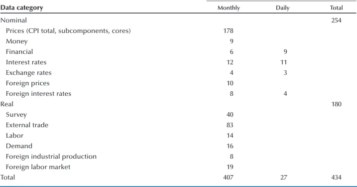
Because we are concerned with the problem of how to weigh the most recent information against what we already know at daily intervals, we are interested in economic data that are fre-quently released, which means working with data with a daily or monthly frequency. Table 1 shows the breakdown of the 434 series into nominal and real variables and their frequency. There are 27 financial variables at the daily frequency and 407 nominal and real variables at the monthly frequency. Quarterly variables such as industrial production or GDP were intentionally excluded to avoid contaminating our estimates with revision errors.4
Two types of panels are constructed. The first uses end-of-month data from 1993:05 to 2003:11; we generate our initial forecasts with this panel. After 2003:11:01, we update the panels daily. The starting date 1993:05 is chosen because a large number of series do not go farther back than 1990 and 1993:05 coincides with a major revision in the CPI.
An explicit intention in constructing the data -set was to transform the series as little as possible. 2
Giannone, Reichlin, and Small (2008) offer an alternative procedure for forecasts of the common component based on the Kalman filter, which are qualitatively the same.
3
Event studies frequently analyze the immediate impact, which is generally defined as the market response 30 minutes before and 30 minutes after the macroeconomic announcement, rather than the full-day impact.
4
See Amstad and Fischer (2009a) for a discussion of data revision at the monthly frequency. Also, preliminary estimates revealed that the introduction of the quarterly information from GDP or industrial production did not alter our estimates.
First, we undertake no seasonal filtering because of its reliance on future information. Amstad and Fischer (2009a) demonstrate that seasonal adjustment can be treated through band-pass fil-tering. The absence of seasonal revisions allows better interpretation of the forecast innovations. Several data transformations, however, were necessary at the initial stages of estimation. The series were filtered in the following manner. First, logarithms were taken for nonnegative series that were not in rates or in percentage units to account for possible heteroskedasticity. Second, the series were first-differenced, if necessary, to account for stochastic trends. Third, the series were taken in deviation from the mean and divided by their standard deviation to remove scalar effects.
Clustered Data Releases
Figure 1 provides an example of the clustering of macroeconomic releases for December 2003. The number of data releases for a particular day is listed on the vertical axis with the calendar
dates denoted on the horizontal axis. The releases are divided into nominal (shaded bars) and real variables (open bars). Of interest are the cluster-ings on December 2 and 19. The first spike stems from CPI releases and their subcomponents, whereas the second is the result of the release of trade volumes across sectors.
APPLICATIONS TO SWISS
INFLATION FORECASTS
This section presents three empirical applica-tions of analyzing the impact of macroeconomic announcement effects on Swiss CPI inflation.5 The case studies were chosen to reflect the view that the event study framework for common-factor 5
The empirical model is defined in Amstad and Fischer (2009a). The same paper provides forecasting properties for a model with 12 static factors and 2 dynamic factors. Inflation is annualized and uses a band-pass filter at 2π/12 to remove seasonality. This is also the same dataset and estimation procedure used to estimate the SNB’s monthly measure of core inflation, called dynamic factor inflation. See page O15 of the SNB’s Monthly Statistical Bulletin.
Table 1
Data and Release Frequencies
Release frequency
Data category Monthly Daily Total
Nominal 254
Prices (CPI total, subcomponents, cores) 178
Money 9
Financial 6 9
Interest rates 12 11
Exchange rates 4 3
Foreign prices 10
Foreign interest rates 8 4
Real 180
Survey 40
External trade 83
Labor 14
Demand 16
Foreign industrial production 8
Foreign labor market 19
models has broad applications. The first exercise considers forecast innovations generated on days when the SNB announced its target range for the 3-month London Interbank Offering Rate (LIBOR) in 2004. In particular, we are interested in how financial variables respond to SNB communica-tion and its impact on the inflacommunica-tion forecast. The second application asks whether forecast innova-tions generated by data releases of real and nomi-nal variables to CPI inflation are synchronized. In other words, do the data releases from real and nominal variables influence the inflation forecast in a similar manner? The last application exam-ines whether forecast innovations generated by import price releases influence CPI inflation. In particular, we want to know whether the impact is similar in magnitude to pass-through ratios estimated in other studies that use traditional time-series methods.
SNB Announcement Surprises in 2004
The SNB defines a target range of 100 basis points for the 3-month LIBOR as its operating target. To steer the LIBOR within the target range, the SNB sets the 1-week repurchase (repo) rate. Four times per year on scheduled dates, the SNB releases a policy statement in which it announces a change or no change in the target range.6In 2004, the announcement dates were March 18, June 17, September 16, and December 16. We use these four policy dates to generate the SNB announce-ment surprises. The SNB “announceannounce-ment surprise” is defined as the one-day difference in the infla-tion forecast condiinfla-tional on postrelease informa-tion minus the inflainforma-tion forecast condiinforma-tional on prerelease information. The difference in this information set captures only information from 6Outside these prearranged dates, the SNB reserves the right to change the target range.
0 50 100 150 200 250 12/02/03 12/05/03 12/08/03 12/11/03 12/14/03 12/17/03 12/20/03 12/23/03 12/26/03 12/29/03 Real Variables Nominal Variables Number of Data Releases
Figure 1
(daily) financial variables and their reaction to the policy statement (i.e., no releases of macro-economic data were made public on the four SNB policy dates). These differences in the panels pertain to daily updates in the 27 financial vari-ables in our panel.
Figure 2 plots innovations of 24-month-ahead inflation forecasts at the time of the four SNB announcement dates. In June and September the SNB’s board of directors raised the target range by 25 basis points, whereas in March and in December the target range was left unchanged. The responses to the SNB announcement surprises differ consid-erably. For the March release, there is no change in the forecast. However, for the dates when the SNB raised its target range, we observe a strong response in the inflation forecast but in opposite directions. Contractionary behavior is observed for the June rate hike and expansionary behavior for the September rate hike. For the last announce-ment surprise in December, we observe a weak but expansionary response to the “no-change” decision. Although the forecast innovations on days when changes to the target range are larger than on days with no changes to the target range, we do not find them to be statistically significant compared with forecast innovations on SNB days in the years between 2000 and 2003. Next, we focus on the direction of the forecast innovation.
How do we explain the differing reactions to the change and no-change decisions in the target range? The release dates that signal a change in the target range account for larger reactions in the inflation forecast. The stronger forecast response on SNB days with a change in the target range rests on the fact that many financial contracts in Switzerland (i.e., automobile leases, home and commercial property loans) are tied to the 3-month LIBOR. To determine the innovation’s direction, it is necessary to control for what the markets had anticipated. As in Hamilton and Jorda (2002), one possible method (aside from the projection one day before the SNB announcement day) is to use a spread of the SNB’s policy rates: the 3-month LIBOR rate minus the repo rate. This interest rate spread is plotted in Figure 3 along with the mid-point in the SNB’s target range for the 3-month LIBOR.7The interest rate spread shows that the
market anticipated the rate hikes in June and September; the spreads widen. For the no-change decisions, the spreads do not change in March and widen slightly before the December policy release.
To understand the postrelease estimate, we need to examine what happens to the spread the day after the SNB policy statements are released. For the March release, the spread does not change between the preforecast and postforecast. This is consistent with the March response of no reaction to the SNB announcement surprises. For the June release, the change in the spread is 0.01, whereas for the September release it is –0.14. In the latter case, the SNB did not raise the repo rates high enough to move the 3-month LIBOR to the mid-point of the target range. In other words, the short end of the yield curve was steeper than was anticipated by the market. This led to a rise in the post -release estimate of inflation. The response to the December release of no change in the target range is similar to the response for the September release. Although the reaction for September is small, the change in the spread for the postrelease and prerelease dates of –0.04 is consistent with the innovation’s direction.
Are Real and Nominal Forecast
Innovations Synchronized?
Next, we test whether forecast innovations from data releases of real and nominal variables are synchronized. We generate the forecast inno-vations from the monthly trade releases (i.e., “real innovations”) and the forecast innovation from the monthly CPI releases (i.e., “nominal innova-tions”). A priori, we do not expect the two types of forecast innovations to be similar. First, the size and dynamics of the individual forecast innova-tions can differ from month to month. Second, the comovement of real and nominal innovations should not be restricted to be the same for each month. In related empirical studies on the pro-cyclicality of prices in the long run, Backus and Kehoe (1992), Ravn and Sola (1995), and Smith (1992) find that the cyclical properties of prices and output are not stable.
7
The repo rate is either the 1-week or the 2-week repo rate; in most cases, it is the former. See Dueker and Fischer (2005).
–3.00E-16 –2.00E-16 –1.00E-16 0.00E+00 1.00E-16 2.00E-16 3.00E-16 4.00E-16 5.00E-16 6.00E-16 1 2 3 4 5 6 7 8 9 10 11 12 13 14 15 16 17 18 19 20 21 22 23 24 –0.04 –0.035 –0.03 –0.025 –0.02 –0.015 –0.01 –0.005 0 –0.002 0 0.002 0.004 0.006 0.008 0.01 0.012 0.014 0.016 0.018 –0.004 –0.002 0 0.002 0.004 0.006 0.008 0.01 0.012
No Change in SNB Target Range: March 18, 2004
25-Basis-Point Raise in SNB Target Range: June 16, 2004
25-Basis-Point Raise in SNB Target Range: September 16, 2004
No Change in SNB Target Range: December 16, 2004
1 2 3 4 5 6 7 8 9 10 11 12 13 14 15 16 17 18 19 20 21 22 23 24
1 2 3 4 5 6 7 8 9 10 11 12 13 14 15 16 17 18 19 20 21 22 23 24
1 2 3 4 5 6 7 8 9 10 11 12 13 14 15 16 17 18 19 20 21 22 23 24 Size of Forecast Innovation
Size of Forecast Innovation Size of Forecast Innovation Size of Forecast Innovation
Figure 2
To test whether the two types of forecast inno-vations are synchronous, we calculate the concor-dance index of Harding and Pagan (2002). The application of the index examines whether the comovement of real and nominal innovations can be quantified by the fraction that both series are simultaneously in the same state of expansion (St= 1) or contraction (St= 0) with the index,
I S tS t S t S t t 1 2 1 2 1 1 1 24 1 1 24 , , , , , , = +
(
)(
)
=∑
– –measuring the degree of concordance between series 1 and 2, which are επr,t+h|k,t and επn,t+h|j,tin our case.8
The concordance index can be used to deter-mine whether nominal and real innovations to inflation are procyclical or countercyclical. If they are exactly procyclical, then the index is unity, whereas a zero value denotes evidence of countercyclical behavior. Table 2 presents the
0 0.1 0.2 0.3 0.4 0.5 0.6 0.7 0.8 01/05/04 02/16/04 03/29/04 05/12/04 06/25/04 08/06/04 09/20/04 11/01/04 12/13/04 Mid-Point of SNB Target Range
3-Month Libor Rate — 1-Week Repo Rate Interest Rate
Figure 3
SNB Policy Rates in 2004
SOURCE: Dueker and Fischer (2005).
Table 2
Synchronization of Forecast Innovations from Nominal and Real Variable Releases
November October September August July June
Forecast innovations 2004 2004 2004 2004 2004 2004 εn π,t+h|j,t, επr,t+h|k,t 0.174 0.348 0.130 0.348 0.826 0.565 εn π,t+h|j,t, επn,t+h|j–1,t 0.522 0.522 0.870 0.822 0.391 0.261 εr π,t+h|k,t, επr,t+h|k–1,t 0.610 0.740 0.565 0.478 0.652 0.434
NOTE: The forecast innovations generated by real and nominal variable releases are denoted by εr
π,t+h|k,tand επn,t+h|j,t. The index for
concordance by Harding and Pagan (2002) lies between 0 (countercyclical) and 1 (procyclical). The index is calculated for the months June through November 2004.
8
The concordance index has similar properties as the Cowles-Jones test used for testing an i.i.d. random walk process.
–0.01 –0.005 0 0.005 0.01 0.015 0.02 0.025
Import Price Shock on CPI Inflation: November 2004
–0.02 –0.015 –0.01 –0.005 0 0.005
Import Price Shock on CPI Inflation: October 2004
–0.025 –0.02 –0.015 –0.01 –0.005 0 0.005 0.01 1 2 3 4 5 6 7 8 9 10 11 12 13 14 15 16 17 18 19 20 21 22 23 24 Import Price Shock on CPI Inflation: September 2004
1 2 3 4 5 6 7 8 9 10 11 12 13 14 15 16 17 18 19 20 21 22 23 24 1 2 3 4 5 6 7 8 9 10 11 12 13 14 15 16 17 18 19 20 21 22 23 24 Size of Forecast Innovation
Size of Forecast Innovation
Size of Forecast Innovation
Figure 4
degree of concordance between επr,t+h|k,tand επn,t+h|j,t for June to November 2004. In the first row of the table, the index values for εr
π,t+h|k,t and ε n
π,t+h|j,t
show that the innovations behaved in a procyclical manner in June and July, but the real and nominal innovations to inflation behaved in a counter-cyclical manner from August through November. In the second and the third rows of the table, infor-mation on the persistence of the innovations is given by constructing the index for επn,t+h|j,tand εn
π,t+h|j–1,t and ε r
π,t+h|k,t and ε r
π,t+h|k–1,t. Here, the
evi-dence shows that the likelihood of the two types of forecast innovations behaving in the same manner (as in the previous month) is stronger for real innovations than for nominal innovations to inflation. In other words, the forecast innovations from realdata releases demonstrate a higher level of persistence than do forecast innovations from
nominaldata releases.
Do Inflation Forecasts Respond to
Releases in Import Prices?
The response of CPI inflation forecasts to import price releases should be informative about the pass through from import prices to consumer prices.9In our setup, the forecast innovation around the import price release is defined as the difference in the 24-month-ahead forecasts in CPI inflation based on the daily panel that includes the postrelease information from import prices and the previous day’s panel that entails infor-mation from the prerelease.
Figure 4 shows the response of CPI inflation to new information from import price releases for November, October, and September 2004. A one-standard-deviation band, based on past innova-tions since December 2003, is depicted around the forecast’s response. The evidence indicates that the pass through under this measure is small. In November and October, the innovations of the import prices were slightly negative for the first 15 months and zero thereafter. The response for September was stronger; again the effect of import prices is absorbed within 18 months.
The finding that the Swiss pass through is
weak in 2004:Q4 does not contradict the cross-country evidence by Campa and Goldberg (2005), Gagnon and Ihrig (2004), and McCarthy (2000). These studies find that the pass through for Swiss prices is surprisingly small compared with the empirical evidence for other small open economies.
CONCLUSION
Understanding the influence of real-time information on inflation forecasts is vital for policymakers. The proposed forecasting frame-work based on the common-factor procedure with daily updated panels is a step in this direction. As in event studies that focus on the response of high-frequency financial data to new information around a narrow event window, the identification scheme herein relies on the recognition that macroeconomic announcement effects can also be interpreted as a forecast innovation with a one-day event window. The case studies for Swiss inflation demonstrate that the event study frame-work for common-factor models is flexible to handle numerous applications in real time.
REFERENCES
Altissimo, Filippo; Bassanetti, Antonio; Cristadoro, Riccardo; Forni, Mario; Hallin, Marc; Lippi, Marco; Reichlin, Lucrezia and Veronese, Giovanni.
“EuroCOIN: A Real Time Coincident Indicator of the Euro Area Business Cycle.” CEPR Discussion Paper No. 3108, Centre for Economic Policy Research, 2001; www.cepr.org/pubs/new-dps/dplist.asp?dpno=3108.
Altissimo, Filippo; Cristadoro, Riccardo; Forni, Mario; Lippi, Marco and Veronese, Giovanni. “New Eurocoin: Tracking Economic Growth in Real Time.” Banca d’ Italia, Temi di discussionedel Servizio Studi No. 631, Bank of Italy, June 2007;
www.bancaditalia.it/pubblicazioni/econo/temidi/ td07/td631_07/td631/en_tema_631.pdf.
Amstad, Marlene and Fischer, Andreas M. “Are Weekly Inflation Forecasts Informative?” Oxford Bulletin of Economics and Statistics, April 2009a, 71(2), pp. 236-52.
9
Amstad, Marlene and Fischer, Andreas M. “Monthly Pass-Through Ratios.” Globalization and Monetary Policy Institute Working Paper No. 26, Federal Reserve Bank of Dallas, January 2009b;
www.dallasfed.org/institute/wpapers/2009/0026.pdf.
Backus, David K. and Kehoe, Patrick J. “International Evidence on the Historical Properties of Business Cycles.” American Economic Review, September 2002, 82(4), pp. 864-88.
Blinder, Alan S.; Ehrmann, Michael; Fratzcher, Marcel; De Haan, Jakob and Jansen, David-Jan. “Central Bank Communication and Monetary Policy: A Survey of Theory and Evidence.” Journal of Economic Literature, December 2008, 46(4), pp. 910-45.
Campa, Jose M. and Goldberg, Linda S. “Exchange Rate Pass-Through into Import Prices.” Review of Economics and Statistics, November 2005, 87(4), pp. 679-90.
Cristadora, Riccardo; Forni, Mario; Reichlin, Lucrezia and Veronese, Giovanni. “A Core Inflation Indicator for the Euro Area.” Journal of Money, Credit, and Banking, June 2005, 37(3), pp. 539-60.
Dueker, Michael J. and Fischer, Andreas M. “Open Mouth Operations: A Swiss Case Study.” Federal Reserve Bank of St. Louis Monetary Trends, January 2005; http://research.stlouisfed.org/publications/
mt/20050101/cover.pdf.
Evans, Martin D.D. “Where Are We Now? Real-Time Estimates of the Macro Economy.” International Journal of Central Banking, September 2005, 1, pp. 127-75.
Forni, Mario; Hallin, Marc; Lippi, Marco and Reichlin, Lucrezia. “The Generalized Dynamic-Factor Model: Identification and Estimation.” Review of Economics and Statistics, 2000, 82(4), pp. 540-54.
Forni, Mario; Hallin, Marc; Lippi, Marco and Reichlin, Lucrezia. “Do Financial Variables Help Inflation and Real Activity in the Euro Area?” Journal of Monetary Economics, 2001, 50(6), pp. 1243-55.
Gagnon, Joseph E. and Ihrig, Jane. “Monetary Policy and Exchange Rate Pass-Through.” International Journal of Finance and Economics, 2004, 9(4), pp. 315-38.
Giannone, Domenico; Reichlin, Lucrezia and Small, David. “Nowcasting: The Real-Time Informational Content of Macroeconomic Data.” Journal of Monetary Economics, May 2008, 55(4), pp. 665-76.
Hamilton, James D. and Jorda, Oscar. “A Model for the Federal Funds Rate Target.” Journal of Political Economy, October 2002, 110(5), pp. 1135-67.
Harding, Don and Pagan, Adrian. “Dissecting the Cycle: A Methodological Investigation.” Journal of Monetary Economics, March 2002, 49(2), pp. 365-81.
MacKinlay, A. Craig. “Event Studies in Economics and Finance.” Journal of Economic Literature, 1997, 35(1), pp. 13-39.
McCarthy, Jonathan. “Pass-Through of Exchange Rates and Import Prices to Domestic Inflation in Some Industrialized Economies.” Staff Report No. 111, Federal Reserve Bank of New York, September 2000; www.ny.frb.org/research/staff_reports/sr111.pdf.
Ravn, Morten O. and Sola, Martin. “Stylized Facts and Regime Changes: Are Prices Procyclical?” Journal of Monetary Economics, December 1995, 36(1), pp. 497-526.
Rigobon, Robert and Sack, Brian. “Noisy Macroeconomic Announcements, Monetary Policy, and Asset Prices,” in John Campbell, ed., Asset Prices and Monetary Policy(NBER). Chap. 8. Chicago: University of Chicago Press, 2008, pp. 335-70.
Smith, R. Todd. “The Cyclical Behavior of Prices.” Journal of Money, Credit, and Banking, November 1992, 24(4), pp. 413-30.
Stock, James H. and Watson, Mark W. “Macroeconomic Forecasting Using Diffusion Indexes.” Journal of Business and Economic Statistics, April 2002, 20(2), pp. 147-61.