Scalable Data Analytics using Spark
A thesis submitted to the
Graduate School of Natural and Applied Sciences
by
Aslan
Bakirov
in partial fulfillment for the
degree of Master of Science
“The way to get started is to quit talking and begin doing. ”
Walt Disney
“It is hard to fail, but it is worse never to have tried to succeed. ”
Scalable Data Analytics using Spark
Aslan
Bakirov
Abstract
This thesis presents our experience in designing a scalable data analytics platform on
top of Apache Spark (major) and Apache Hadoop (minor). We worked on three
repre-sentative applications: (1) Sentiment Analysis, (2) Collaborative Filtering and (3) Topic
Modeling. We demonstrated how to scale these applications on a cluster of 8 workers.
Each worker contributes 4 cores, 8 GB RAM, and 100 GB of disk space to the
com-pute pool. Our conclusion is that Apache Spark has enough maturity to be deployed in
production comfortably.
Collabo-Spark Kullanarak Ölçeklenebilir Veri Analitiği
Aslan
Bakirov
Öz
Bu tez calışmasında, Apache Spark ve Apache Hadoop platformları üzerinde
ölçek-lenebilir veri analitiği çalışılmıştır. Temel olarak üç tane temsili uygulama geliştirilmiştir:
(1) Duygu Analizi, (2) İşbirliğine Dayalı Filtreleme ve (3) Konu Modellemesi. Bu
uygu-lamaların 8 makinelik bir küme üzerinde ölçeklenebilirliği gösterilmiştir. Her makine
hesaplama havuzuna 4 çekirdek, 8 GB RAM ve 100 GB disk alanı kadar katkıda
bu-lunmuştur. Gözlemlerimize göre, Apache Spark üretim ortamlarında güvenli bir şekilde
kullanılabilir olgunluktadır.
Anahtar Sözcükler:
Ölçeklenebilirlik, Duygu Analizi, İşbirliğine Dayalı Filtreleme,
Konu Modellemesi
Acknowledgments
I would like to express my deepest appreciation to my advisor Prof. Ahmet Bulut.
His patience, knowledge and vision has great affect on this dissertation and on my life.
Without his guidance and persistent help, this dissertation would not have been possible.
I would also like to deeply thank my jury members, Prof. Ali Çakmak and Prof. İsmail
Arı for their time, insightful comments, and their support.
I would like to greatly acknowledge and thank the friendly staff of College of Engineering
and Natural Sciences and, in particular, Seçil Öcal for creating a friendly environment
to conduct research.
I would also like to thank my friends, especially Kevser Nur Çoğalmış, for all the great
study times we had together during my stay at this university.
This thesis is supported by Turkish National Science Foundation (Tübitak) under grant
numbers 113E243 and 113E622 and Turk Telekom Argela under Grant Number 6401-01.
Contents
Abstract
ii
Öz
iii
Acknowledgments
v
List of Figures
viii
List of Tables
ix
1
Introduction
1
2
Sentiment Analytics on Spark
2
2.1
Related Work . . . .
2
2.2
Methodology
. . . .
3
2.2.1
Preprocessing on the data . . . .
3
2.2.2
Naive Bayes Classifier . . . .
3
2.3
Experimental Setup
. . . .
5
2.3.1
Resilient Distributed Datasets(RDD) . . . .
5
2.3.2
Broadcast Variables
. . . .
6
2.3.3
The Movie Reviews Dataset . . . .
6
2.3.4
Cluster Configuration
. . . .
7
2.3.5
Model Building . . . .
8
2.4
Experimental Evaluation . . . .
9
2.4.1
Apache Hadoop . . . .
9
2.4.2
Apache Mahout . . . .
9
2.4.3
Empirical Results . . . .
10
2.4.3.1
Broadcasting vs. Not-broadcasting . . . .
10
2.4.3.2
Time required for training . . . .
10
2.4.3.3
Time required for testing . . . .
11
3
Collaborative Filtering on Spark
13
3.1
MLBase . . . .
13
3.2
System Architecture . . . .
14
3.3
Online Recommendation System
. . . .
14
4
Topic Modeling on Hadoop
17
4.1
Introduction . . . .
17
Contents
vii
4.3
LDA in MapReduce
. . . .
18
4.4
Experimental Results . . . .
19
4.4.1
The Dataset . . . .
19
4.4.2
Cluster Configuration
. . . .
19
4.4.3
Test Results . . . .
19
5
Conclusions
22
Bibliography
23
List of Figures
2.1
Şehir cluster. . . .
8
2.2
Runtime chart of testing step with broadcast and without broadcast. . . .
11
2.3
Runtime chart of testing step on Spark vs. Hadoop hosted in the Şehir
cluster in minutes. . . .
12
3.1
Şehir Cluster System Architecture for Recommendation Application. . . .
14
3.2
Şehir Cluster System Workflow for Recommendation Application. . . .
16
3.3
MLBase Architecture. . . .
16
List of Tables
2.1
Reviews augmented with sentiment.
. . . .
4
2.2
Reviews augmented with sentiment.
. . . .
4
2.3
Words and their class frequency.
. . . .
4
2.4
Description of the test data. . . .
7
2.5
The running time of the testing step on Spark (in minutes) hosted in the
Amazon EC2 cluster. . . .
10
2.6
Runtime of the training step on the Şehir cluster. . . .
10
2.7
The running time of the testing step for Mahout’s Naive Bayes Classifier
(in seconds) hosted in the Şehir cluster.
. . . .
11
2.8
Runtime comparison of the testing step on Hadoop and Spark hosted in
the Şehir cluster in minutes. . . .
12
3.1
Online Recommendation Data. . . .
15
3.2
Prediction matrix of ALS algorithm. . . .
15
4.1
LDA runtime on unigrams of
51168
documents. . . .
20
4.2
LDA runtime on bigrams of
51168
documents. . . .
20
4.3
LDA runtime on Amazon Movie Reviews Data. . . .
20
4.4
The analysis of LDA’s computation time with varying number of nodes
and with varying number of documents. . . .
20
Chapter 1
Introduction
With the advent of social networks, forums, and blogs, amount of data on the Web has
increased rapidly resulting in an information explosion. Internet users make purchases
online, listen to music, or watch a movie; later on, they make comments about their
purchases, indicate their musical preference, and write their opinions about movies they
recently watched. Raw user data does not provide much information unless information
is explicitly cultivated. Data mining refers to the process of extracting information from
raw data.
Data mining is used for a variety of information discovery tasks such as
classification, clustering, and regression. Since actual task implementations analyze the
entire set of data in order to find a pattern, the run time of these algorithms depend on
the size of the dataset. Handling large amounts of data requires the use of MapReduce
(M/R) programming model on special purpose compute clouds. Hadoop was one of the
first platforms to provide an implementation of M/R on a compute cluster. A relatively
new implementation of M/R called Spark has been shown to provide performance benefits
of up to ten times compared to Hadoop on certain machine learning tasks [1].
In this thesis, three representative applications of distributed machine learning are
stud-ied. The first application is for extracting sentiment from movie reviews by using a Naive
Bayes Classifier. The second one is a recommendation system, which uses collaborative
filtering. The third and the last application is topic modeling with latent dirichlet
allo-cation (LDA). In the first two appliallo-cations, Apache Spark was benchmarked in different
scenarios. The last application is about benchmarking LDA on Apache Hadoop.
Chapter 2
Sentiment Analytics on Spark
Naive Bayes Classifier is used to extract text sentiment. We trained our model by using
Spark, Hadoop and Apache Mahout and tested with different data sizes and cluster
configurations. We compared the performance of the Naive Bayes Text classifier on
Apache Spark, Apache Hadoop and Apach Mahout. We implemented the classifiers on
Apache Spark and Apache Hadoop ourselves [2].
2.1
Related Work
Pang et al. [3] used the IMDB movie dataset for sentiment analysis. They used naive
bayes, maximum entropy, and support vector machine (SVM) for classification. However,
their study was done on a single compute node, and does not address how to scale
computation as the data itself scales. The text features extracted included bag of words,
bigrams, and part of speech tags. Their study showed that SVM with unigram features
had the best performance. Elsayed et al. [4] proposed an M/R algorithm for finding
pairwise document similarity for large document collections. They used a cluster of 19
worker machines with dual core, 4 GB of memory, and 100 GB of disk space each. Their
algorithm was implemented as two M/R jobs: the first job was used to index documents
for finding out list of document IDs that contain a given term and associated term weight.
The second job was used to calculate pairwise similarity scores. The experiments showed
that the running time of their approach scaled linearly with the number of documents.
Khuc et al. [5] provided a method for analyzing sentiment on twitter data using Hadoop.
The authors created their own lexicon suitable for tweets, which included emoticons.
They used lexicon as the first classifier and logistic regression as the second classifier.
Their experiment was done on 5 nodes in Amazon EC2 cluster with 2 virtual cores and 1.7
GB of memory. An experiment to create the lexicon was carried out on 100K, 200K and
Chapter 2.
Sentiment Analytics on Spark
3
300K tweets. For the 300K-scenario, it took 600 minutes to build a lexicon on 5 machines.
Their lexicon-and-learning-based classifier took 20 minutes to analyze the sentiment of
2.5 million tweets. Hunter et al. [6] migrated their millennium traffic project from a
single machine to multiple machines. They used Spark as it allows M/R and iterative
algorithms at the same time. A special purpose data structure called resilient distributed
data is used to share large data items between cluster machines for collaboration. The
migration to Spark improved the run time of their system by 2.8 times.
2.2
Methodology
2.2.1
Preprocessing on the data
For downstream tasks that expect meaningful and cleaned-up data, the dataset is
pre-processed as follows:
•
All text is lowercased.
•
Punctuation symbols are removed.
•
Hyphened word groups are separated.
•
Stop-words such as “a, an, the, they, so, much” are removed using the natural
language toolkit called NLTK [7].
•
HTML tags are removed.
•
In the original dataset, the score information is numeric and is in the range of [1.0,
5.0]. As a pre-processing step, a review is categorized as negative if its review score
is less than 3.0; otherwise (if its review score is greater than or equal to 3.0) it is
categorized as positive.
2.2.2
Naive Bayes Classifier
Naive Bayes is one of the simplest machine learning algorithms used in text classification.
The Bayesian formula is [8];
P
(
C
=
c
k|
X
=
x
) =
P
(
C
=
c
k)
×
P
(
X
=
x
|
C
=
c
k)
P
(
x
)
(2.1)
Chapter 2.
Sentiment Analytics on Spark
4
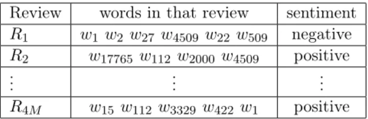
computed, i.e., one per class. Each text consists of a set of words
w
ias shown in Table
2.1.
Table 2.1: Reviews augmented with sentiment.
Review
words in that review
score
R
1w
1w
2w
27w
4509w
22w
5092.0
R
2w
17765w
112w
2000w
45095.0
..
.
..
.
..
.
R
4Mw
15w
112w
3329w
422w
14.0
During the pre-processing, every review is assigned to a class. A review having a score less
than 3.0 is tagged as negative; otherwise it is assigned to the positive class. Therefore,
the reviews are converted into new structures as shown in Table 2.2.
Table 2.2: Reviews augmented with sentiment.
Review
words in that review
sentiment
R
1w
1w
2w
27w
4509w
22w
509negative
R
2w
17765w
112w
2000w
4509positive
..
.
..
.
..
.
R
4Mw
15w
112w
3329w
422w
1positive
The training set consists of 4 million texts. Out of this 4 million, there are 2.4 million
in the positive class and 1.6 million in the negative class. For each word, two counts
are computed and stored: the first count represents the number of positive reviews that
contain the word, and the second count represents the number of negative reviews that
contain the word as in Table 2.3.
Table 2.3: Words and their class frequency.
Word
positive reviews
negative reviews
w
145600
120000
w
272250
50000
w
322500
69900
..
.
..
.
..
.
w
4390400
23220
Chapter 2.
Sentiment Analytics on Spark
5
The formula in Equation 2.1 is applied to each sentence in the test dataset in order to
predict whether the sentence belongs to the positive or to the negative class. Suppose
that a review R in the test dataset corresponds to
w
1, w
2, w
43. For R, the probability of
being in either class is computed as follows:
p(C= +|R) =p(C= +)×p(w1|C= +)×p(w2|C= +)×p(w43|C= +) = 2400000 4000000× 45600 2400000× 72250 2400000 × 90400 2400000 = 0,00001288 (2.2)
Probability of being in “positive” class
p(C=−|R) =p(C=−)×p(w1|C=−)×p(w2|C=−)×p(w43|C=−) = 1600000 4000000× 120000 1600000 × 50000 1600000 × 23220 1600000 = 0.00002024 (2.3)
Probability of being in “negative” class
The text sentiment is classified as the class that has a greater probability value. In the above example, the text sentiment forRis attributed to negative.
2.3
Experimental Setup
In Spark, jobs are submitted for processing a large dataset [1]. Each job first loads its working data into memory for enabling rapid data access. The main component of Spark is the construct of a resilient distributed dataset (RDD).
2.3.1
Resilient Distributed Datasets(RDD)
A resilient distributed dataset provides granular fault tolerance and distribution of work. An input data is sliced into multiple chunks so that parallel jobs can be executed on each chunk. Storing lineage information in the framework per RDD provides fault tolerance. Each compute step in the compute flow can be re-executed linearly to enable recovery in case of failures. Paral-lelized collections and Hadoop datasets are two ways to create an RDD. ParalParal-lelized collection is a wrapper on Scala programming language’s collection, which also supports parallel operations. It can be created by calling the parallelize method of Spark Context on an existing Scala collec-tion. Parallelized collections and Hadoop datasets are two current forms of RDD. Parallelized collection is a wrapper on Scala collection, which also supports parallel operations. This form of RDD can be created by calling a parallelize method of Spark Context on existing Scala collection.
val data = Array(1, 2, 3, 4, 5) // data is typical Scala collection. val distData = sc.parallelize(data) // distData is an RDD.
Chapter 2.
Sentiment Analytics on Spark
6
an RDD by calling textFile method of Spark Context as follows:
val distFile = sc.textFile(“hdfs://.../data.txt”)
Two types of operations can be done on RDDs: transformations and actions. An RDD can be transformed into another RDD by using a mapper. An action corresponds to an aggrega-tion used during reducaggrega-tion. Spark currently provides three APIs, one for each of Scala, Java, and Python programming languages. We used the Java API. We have a dictionary holding the number of occurrence of each word in each of positive and negative classes. This “read-only” data is used to compute the sentiment of a given review as explained in 2.2.2. Since Spark is a distributed environment, each node must be able to make a lookup in this read-only dictio-nary. Spark’s default behavior is to send the required data within the compute cluster before each iteration. The default behavior results in a bottleneck in the master node and its available bandwidth, and therefore limits scalability. Our solution to this problem is to use the broadcast variables of Spark framework.
2.3.2
Broadcast Variables
Broadcast enables us to send a map to worker nodes only once at the beginning of the job execution. We can share the maps that hold occurrence counts per category with the use of the broadcast feature in Spark. In order to test this feature, we implemented two methods in order to perform data lookups:
i When any worker needs data and if that data resides in another node in the cluster, the data owner sends the requested data to the requestor. This operation consumes less random access memory (RAM), but requires high IO and CPU operations.
ii We can store lookup tables in full in all workers. This approach requires more RAM for data storage, but it needs less IO. This method can be accomplished by broadcasting lookup dictionaries to all worker nodes as follows:
Broadcast<JavaPairRDD<String, Double>> posMapBroadcast
= sc.broadcast(positiveDataMapRDD);
Here, “positiveDataMapRDD” is the original data structure and “posMapBroadcast” is the new data version that will be broadcasted to each node. By using broadcast variables, we optimized our computation time by 1.15 times.
2.3.3
The Movie Reviews Dataset
In experiments, Amazon movie reviews [9] were used. There were 7,911,684 reviews, which were extracted from 889,176 reviews for 253,059 products. Some reviews contain a single sentence,
Chapter 2.
Sentiment Analytics on Spark
7
while some others contain more than ten sentences. The median number of words per review is 101. All reviews have information about product ID, user ID, time, score, summary, and text. An example review is given below:
• product/productId: B00006HAXW • review/userId: A1RSDE90N6RSZF • review/profileName: Joseph M. Kotow • review/helpfulness: 9/9
• review/score: 5.0
• review/time: 1042502400
• review/summary: Pittsburgh - Home of the OLDIES review/text: I have all of the doo wop DVD’s and this one is as good or better than the 1st ones. Remember once these performers are gone, we’ll never get to see them again. Rhino did an excellent job and if you like or love doo wop and Rock n Roll you’ll LOVE this DVD !!
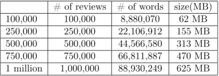
Only the score and summary information above were used in our system. After the pre-processing, the sentiment label for each review was added to the end of each entry separated by a comma. The entire dataset was separated into two parts as the training set and the test set. The training set consisted of 4 million reviews, which had about 349,993,900 words. The rest of the dataset was used as the test set. Five different test configurations were constructed with 100,000, 250,000, 500,000, 750,000, and 1 million reviews respectively. Table 2.4 gives detailed information about the test data.
Table 2.4: Description of the test data.
# of reviews
# of words
size(MB)
100,000
100,000
8,880,070
62 MB
250,000
250,000
22,106,912
155 MB
500,000
500,000
44,566,580
313 MB
750,000
750,000
66,811,887
470 MB
1 million
1,000,000
88,930,249
625 MB
2.3.4
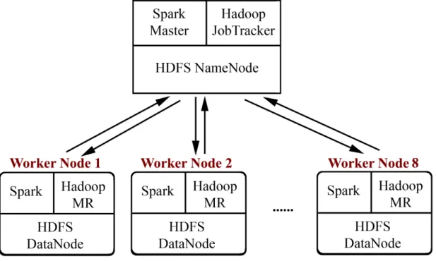
Cluster Configuration
Two different clusters were used for performance comparison. The first cluster called Şehir Cluster has one master and 8 workers with 4 cores CPU, 8 GB of RAM, and 100 GB of disk space. The Şehir cluster is depicted in Figure 2.1. The second cluster called Amazon Cluster hosted in Amazon EC2 has one master and 4 workers with 4 cores CPU and 15 GB of RAM. The Java Development Kit version 1.7.0_03 was installed on each node for a Java Runtime Environment in both clusters. Since the dataset is large, the Hadoop Distributed File System (HDFS) was chosen to store this data. The HDFS version 1.0.4 was installed in the clusters. On
Chapter 2.
Sentiment Analytics on Spark
8
Figure 2.1: Şehir cluster.
2.3.5
Model Building
For training, two map jobs and two reduce jobs were created: one M/R job pair was created for the positive class and the other M/R pair was created for the negative class. In the mapping stage, each review was mapped to either the negative class or the positive class. For both classes, a separate word counts dictionary was created. This action resulted in a positiveMap and a neg-ativeMap. Each sentence of a review was split by whitespace into individual words. Every word was mapped into a value of “1” keyed by the word itself. In the reduce step, all values were summed up per key. After the job completed, the information as to how many positive and how many negative reviews a given word occurred in were computed. In order to outline how our M/R works, let us demonstrate how to compute the positive class probability for a given review R, which consists of wordsw1, w2, . . . , wn. 1
Map (M):
i. Each word is mapped to(R,1)as its value, i.e.,(wi,(R,1))wherei= 1, . . . , n.
ii. This (key, value) tuple is joined with positive lookup map, which has words askeyand the number occurrences of those words in positive reviews as the correspondingvalues. In the positive lookup map, an entry looks like(wi, X), where X is a positive integer that holds
the total number of occurrences ofwi in positive reviews.
iii. After the join, the interim results map has the following (key, value) pairs(wi,((r,1), Xi))
wherei= 1, . . . , n. 1
Chapter 2.
Sentiment Analytics on Spark
9
iv. We swap the places ofRandwiin each of these tuples to finally get(R,((wi,1), Xi))where
i= 1, . . . , n.
Reduce(R):
i. Each entry is then reduced by using reduceByKey function as follows:
(R, X1 N umP os× X2 N umP os×. . .× Xi N umP os) =Y
ii. The tuple(R, Y × N umP os × N umT otalDocuments)represents the final result(K, V). The key K is the review R itself, and the value V corresponds to the probability of R belonging to the positive class.
2.4
Experimental Evaluation
We compared our solution with two alternatives. Both of the alternative approaches were based on Hadoop: (i) a naive bayes classifier built using Hadoop M/R and (ii) another naive bayes classifier built using Apache Mahout. We describe these two frameworks next before presenting our empirical findings.
2.4.1
Apache Hadoop
Hadoop is an Apache foundation framework that can be used for processing large data sets on a cluster of computers using M/R programming model [10]. The two main projects of Hadoop are the Hadoop Distributed File System (HDFS) and Hadoop M/R. The HDFS is a fault tolerant, scalable, and highly configurable distributed file system written in Java. An HDFS cluster has a master name node that manages synchronization and coordination among data nodes, and stores metadata for the cluster. Multiple data nodes store the actual user data. An HDFS client contacts the name node for file operations such as select, insert, and delete. The HDFS also has support for failing over to a secondary name node in order to avoid the single master being the single point of failure. The Hadoop M/R enables programmers for writing applications in order to process large datasets in parallel on a cluster of machines. An M/R job has two main components: (1) map and (2) reduce. The framework splits input data into multiple chunks so that multiple map tasks can process these individual data partitions in parallel. Outputs of the map tasks are collected and processed by the subsequent reduce tasks. The inputs and the outputs of each job are stored in the HDFS. Since the map and the reduce tasks operate on < key, value >pairs, the input and output format will also be< key, value >pairs.
2.4.2
Apache Mahout
li-Chapter 2.
Sentiment Analytics on Spark
10
constructing random forests, and recommending items. All these end-user products are imple-mented on top of Hadoop. Since Mahout has naive Bayes classifier support, we included it in our tests. During training, Mahout created a handful of feature vector output files and built a final model from these interim output files. The whole process took almost three hours. During testing, the model built was used on the same test dataset that was used in the other competing approaches.
2.4.3
Empirical Results
2.4.3.1
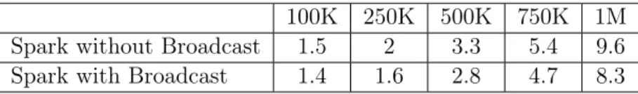
Broadcasting vs. Not-broadcasting
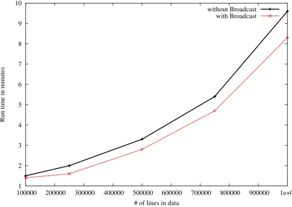
In order to see the effect of broadcasting vs. relying on the framework to shuffle data when it is needed, we conducted an experiment on five test scenarios. This test was done on the Amazon cluster. As shown in the results in Table 2.5 and Figure 2.2, the broadcast method took less time to go through the testing phase. On 1M reviews, the method with broadcasting completed 1.3 minutes faster than the method without broadcasting. The reason for this improvement is that the application driver did not waste time trying to share the required data among the compute nodes as the alternative approach did. The gap in running time widened between the two methods as the size of the data increased. This is because the increased data size led to the increased data delivery between the compute nodes.
Table 2.5: The running time of the testing step on Spark (in minutes) hosted in the Amazon EC2 cluster.
100K
250K
500K
750K
1M
Spark without Broadcast
1.5
2
3.3
5.4
9.6
Spark with Broadcast
1.4
1.6
2.8
4.7
8.3
2.4.3.2
Time required for training
On the Şehir cluster, we conducted two tests: one using 4 workers and the other using 8 workers. Table 2.6 shows how long it took to train on Spark vs. Hadoop with different number of workers. The training time in case of Hadoop was in the order of minutes, while training using Spark was in the order of seconds.
Table 2.6: Runtime of the training step on the Şehir cluster.
4 Workers
8 Workers
Hadoop
12 minutes
10 minutes
Spark
73 seconds
62 seconds
Chapter 2.
Sentiment Analytics on Spark
11
1 2 3 4 5 6 7 8 9 10 100000 200000 300000 400000 500000 600000 700000 800000 900000 1e+06Run time in minutes
# of lines in data
without Broadcast with Broadcast
Figure 2.2: Runtime chart of testing step with broadcast and without broadcast.
2.4.3.3
Time required for testing
Table 2.8 and Figure 2.3 show the run time of the testing step on Hadoop and Spark on the Şehir cluster. Compared to Hadoop on all test scenarios, Spark implementation was up to 10 times faster in crunching data. For example, on 1 million reviews with 8 workers, Spark completed the testing in 7.9 minutes while Hadoop implementation required 70 minutes to complete. The benefits of using the broadcast variables were even more apparent in the Şehir cluster. Using 4 workers only, 750K reviews were digested in 8.6 minutes with broadcasting compared to 11 minutes without it. The results for Mahout are shown in Table 2.7.
Table 2.7: The running time of the testing step for Mahout’s Naive Bayes Classifier (in seconds) hosted in the Şehir cluster.
#
of reviews
4 Workers
8 Workers
100K
63
66
250K
75
60
500K
101
77
750K
112
82
1M
150
112
Chapter 2.
Sentiment Analytics on Spark
12
in the cluster. The advantage of a high number of compute nodes in a cluster did not justify itself, because the dataset size was not large enough. For larger data sizes, the benefit of using a higher number of workers was more apparent. For example, it took 112 seconds to digest 1 million reviews with 8 workers, while it took 150 seconds with 4 workers.
Table 2.8: Runtime comparison of the testing step on Hadoop and Spark hosted in the Şehir cluster in minutes.
4 Workers
8 Workers
Spark
Hadoop
Spark
Hadoop
w/oB
1wB
2Dist.
3w/oB
wB
Dist.
100K
1.8
1.6
13.1
1.9
1.6
15.4
250K
2.6
2.2
22.5
2.4
2.1
24.2
500K
4.6
3.5
33.3
3.3
2.6
36
750K
11.0
8.6
58.3
5.3
4.0
50
1M
OoM
4OoM
78.5
8.9
7.9
70
1 without Broadcast 2 with Broadcast 3 Distributed Cache4 Out of Memory Exception: This exception occurs when program runs
out of memory. When our task starts running, our working data is loaded to the cache. Since the number of reviews up to 1M, data size increases. Since join operation is costly because Cartesian product with lookup Map, extra 250K reviews run our program out of memory.
0 10 20 30 40 50 60 70 80 100000 200000 300000 400000 500000 600000 700000 800000 900000 1e+06
Run time in minutes
# of lines in data
Spark without Broadcast 4W Spark with Broadcast 4W Hadoop Distributed Cache 4W Spark Without Broadcast 8W Spark with Broadcast 8W Hadoop Distributed Cache 8W
Figure 2.3: Runtime chart of testing step on Spark vs. Hadoop hosted in the Şehir cluster in minutes.
Chapter 3
Collaborative Filtering on Spark
In this chapter, we give the details of our reference system that consumes the recommendations computed using Apache Spark’s MLBase library [12]. The reference system stands for an entire Web 2.0 service, which serves vital data from an in-memory cache layer. The cache layer is bootstrapped with recommendations computed a-priori by the backend batch processing engine powered by Apache Spark.
3.1
MLBase
MLBase is scalable machine learning framework that runs on Apache Spark Engine. MLbase consists of three components – MLlib, MLI, and ML Optimizer.
1. ML (Machine Learning) Optimizerautomates the task of ML pipeline construction. It optimizes algorithm parameters and data sampling at runtime. Moreover, the optimizer estimates execution time and algorithm performance based on statistical models built using the statistics from previous jobs.
2. MLI (Machine Learning Interface) is an API for feature extraction and algorithm development that introduces high-level ML programming abstractions.
3. MLlib (Machine Learning Library)is a distributed machine learning library that runs on Spark.
Developing scalable machine learning algorithms using MLI is very simple. For instance, the following code block builds a model for recommending movies.
var X = load("user_movie_pairs", 1 to 2) var y = load("user_ratings", 1)
var (fn-model, summary) = doCollabFilter(X, y)
Chapter 3.
Collaborative Filtering on Spark
14
3.2
System Architecture
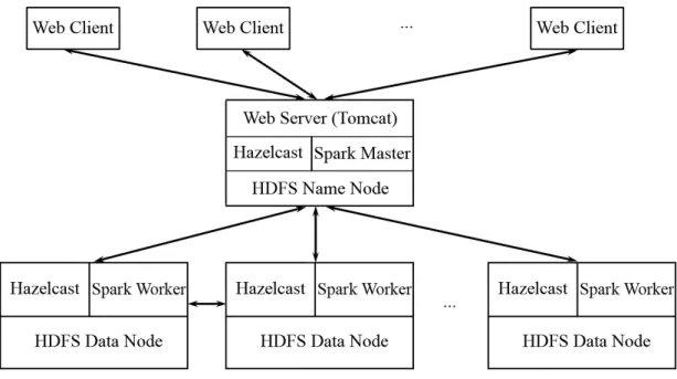
Training data is stored in HDFS. We used MLBase for building a prediction model on top of this data. The model is stored in a distributed cache, which forms our Hazelcast layer [13]. Hazelcast is an open source in-memory data grid written in Java. Data can be distributed evenly across cluster. For avoiding data loss and handling fault, replicas of data is also distributed among nodes. There are different use cases of Hazelcast. Three widely used scenarios are:
• distributed cache, often in front of a database, • clustering web sessions, and
• Map Reduce API for in memory big data processing and analytics.
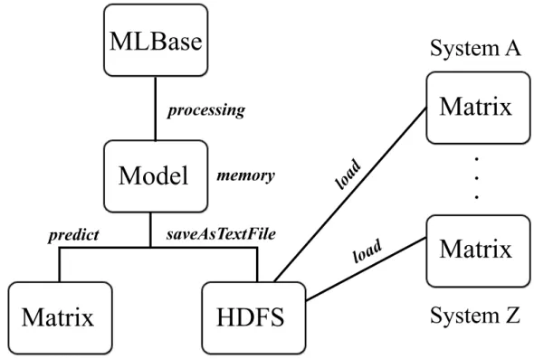
The topmost layer is our web layer, which serves users with movie recommendations. The full architecture is shown in Figure 3.1.
Figure 3.1: Şehir Cluster System Architecture for Recommendation Application.
3.3
Online Recommendation System
For the online recommendation system, we used the movie review dataset, which was used in Chapter 2. We used information of user id, product id and the score given by user id to product id. Table 3.1 shows a data sample.
Chapter 3.
Collaborative Filtering on Spark
15
Table 3.1: Online Recommendation Data.
User ID
Product ID
Score
26256
208865
3.0
484047
208865
3.0
118779
208865
5.0
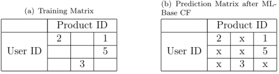
We used ALS (alternative least squares) of MLI for training a recommender from training data (which 500,000 user id, product id, and score entries). The algorithm predicts the empty cells using the partial data as shown in Table 3.2. All predictions are written as a matrix in the HDFS. When the web server is up, the Hazelcast cluster loads prediction matrix from HDFS to main memory. We recommend top products to each user based on the prediction scores. After a user is logged in, personal recommendations are shown in a matter of seconds. Filling the matrix from 500,000 entries took 6 minutes.
Table 3.2: Prediction matrix of ALS algorithm.
(a) Training Matrix
Product ID
User ID
2
1
5
3
(b) Prediction Matrix after ML-Base CF
Product ID
User ID
2
x
1
x
x
5
x
3
x
At the beginning, we only have unstructured raw big data. Since MLI interface accepts input data in a particular format to build a model, we have to parse the raw data to the desired format and persist to HDFS. Then, we build a model using MLI and fill the prediction matrix by using the model. When the web server is up, the Hazelcast cluster loads all recommendations to the memory for web server to be able to serve recommendations online. The system workflow is shown in Figure 3.2.
Building a model from scratch is resource and time consuming. The framework supports saving the model on to the HDFS. This enables us to use the model later on and also make it usable
Chapter 3.
Collaborative Filtering on Spark
16
Figure 3.2: Şehir Cluster System Workflow for Recommendation Application.
Chapter 4
Topic Modeling on Hadoop
4.1
Introduction
With our fast adoption of technology, our lives have become more digital. We read daily news online, track daily blogs to follow trends, and do a dozen Internet searches per day. The Internet is ever growing with images, videos, articles, books, blogs, and wikis. With the increasing number of resources on the Internet, now it gets more difficult to find what we are looking for on the Internet. Although search engines help finding desired information by matching queries with the information which seems related, humans do a fair share by filtering out the seeds from the chaff. This is where topic modeling can help eliminate irrelevant results.
Identifying topics in a text collection helps us organise the collection around similarities between documents and themes. In order to categorize documents, one can use clustering, LDA, or probabilistic latent semantic analysis (pLSA) among many. In clustering, each document is categorized under a single cluster, which is a limitation in scenarios where documents can contain more than one theme. LDA on the other hand can classify a document under more than one topic. LDA is an iterative algorithm based on coordinate ascent, and unfortunately it requires ample time to converge to a final set of topics. In order to reduce time to convergence, we developed LDA on Hadoop and tested its performance on sizeable text collections.
4.2
Related Work
In LDA, each document is represented as a probability distribution over topics. Each topic is represented as a probability distribution over words in a chosen vocabulary. In order to re-create a text collection from its topic model, a generative process can be devised as follows: for each word of a document, choose a topic according to the topic distribution of that document, and then choose a word from the word distribution of that topic. This process is repeated for all documents.
Chapter 4.
Topic Modeling on Hadoop
18
Misra et al. used LDA for segmenting text, i.e., dividing text into topically coherent parts [14]. Their assumption was that a change in concept can be due to a change in topic. Hong et al. used LDA for finding topics in Twitter [15]. They combined text found in user profiles with the actual tweets. Their findings were that document length affected the model accuracy and that the model worked better on short documents specifically in tweet categorization.
Wang et al. used LDA in order to improve collaborative filtering for recommending scientific articles to scholars [16]. Traditional recommendation systems for this purpose use collaborative filtering, which are based on the ratings of users. However, this approach ends up recommending old articles while ignoring new scientific articles or the ones which are published recently and have not been rated yet. In order to alleviate this drawback, the text content were taken into account in collaborative filtering with content bits provided by the LDA itself.
Tang et al. used topic modelling in order to formulate the relationship between authors, papers and venues for making academic search results more relevant [17]. They named their model as Author-Conference-Topic (ACT) model. Each article was represented by a vector of words, a vector of authors and a vector of venues. Their LDA based ACT model outperformed other legacy systems in use.
4.3
LDA in MapReduce
Probabilistic topic modeling is used to discover and annotate large archives of documents with thematic information [18]. With an increasing number of news, scientific articles, books, blogs, and web pages, it gets more difficult to categorize and search among the wealth of information. The idea behind LDA is to model documents as being generated from multiple topics (e.g., K topics) such that each of these topics is a probability distribution over a pre-defined vocabulary. Each document in the corpus exhibits topics in different proportions. In order to learn word distributions per topic and topic proportions per document, posterior probabilistic inference is used. With the observed documents in the corpus as output, hidden topical structure can be inferred by a deterministic variational method.
Variational methods posits a parameterised family of distributions such as Dirichlet over the hidden structure and learn the parameters that maximise the log likelihood of the observations under the model. In the variational inference procedure, a simpler distribution that contains free variational parameters is used to approximate the true posterior distribution. There are three sets of hidden variables each of which is governed by a different variational parameter: (1) a word distribution per topic, (2) a topic distribution per document, and (3) word-to-topic assignment per document [19]. All variables are assumed to be independent of each other. The variational parameters that maximize the log likelihood of the observations under the model are computed iteratively by continuous optimization using coordinate ascent.
In the setup method before starting mappers, we load the variables stored in the distributed cache and normalise λs for each topic before the start of an iteration. The distributed cache
Chapter 4.
Topic Modeling on Hadoop
19
is a distributed hashmap where multipleclients from different JVMs can put and fetch values concurrently.
In the mapper phase, when MapReduce job starts,λandγare initialised randomly. The hyper-parameter αis constant and is set to0.5. In the subsequent iterations, each mapper task loads the latest values of the free parameters from the distributed cache, updatesλs andγs, and stores them in the distributed cache. They are also transmitted from the mappers to the reducers via the same cache.
In the reduce phase, we update λandαand put them back in the cache for the next iteration [20].
4.4
Experimental Results
4.4.1
The Dataset
Three different datasets were used in the experiments. The first dataset was used to examine accuracy. This dataset contains search keywords of an advertisement campaign. In total, there are51168keywords.
The second dataset used was Amazon movie reviews was used in Chapter 1 and Chapter 2. The total number of words in the whole collection is431,236,979. The attributes per review are product ID, user ID, time, score, summary, and text. We only used text field in our experiments.
The third dataset belongs to David Blei’s research [21]. The original dataset has2246documents. We created four data subsets from the original one in order to show how LDA scales with number of nodes in the cluster and with document size.
4.4.2
Cluster Configuration
We used a cluster of one master and8workers each with4cores,8GB of RAM, and100GB of disk space. The Java Development Kit version 1.7.0_03 was installed on each node as the Java Runtime Environment. The HDFS version 2.5.0 was installed in the cluster.
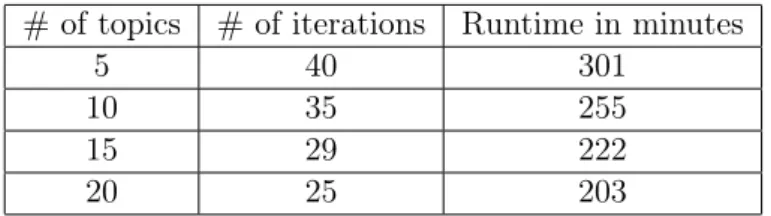
The optimization was allowed to run for 40 iterations at maximum and the number of topics varied from 5 to 20. In case the log likelihood criterion for the optimization is met before the maximum number of iterations is reached, the process is stopped forcefully.
4.4.3
Test Results
In the set of experiments conducted on the first dataset, the number of iterations and the computation time were measured for varying number of topics. In case of a vocabulary of
Chapter 4.
Topic Modeling on Hadoop
20
while the number of topics increased from5to20. However in case of a vocabulary of bigrams1, the number of iterations and the runtime had no clear trend as shown in Table 4.2.
Table 4.1: LDA runtime on unigrams of51168documents.
#
of topics
#
of iterations
Runtime in minutes
5
40
301
10
35
255
15
29
222
20
25
203
Table 4.2: LDA runtime on bigrams of51168documents.
#
of topics
#
of iterations
Runtime in minutes
5
40
279
10
38
281
15
30
219
20
37
291
Table 4.3: LDA runtime on Amazon Movie Reviews Data.
#
of topics
#
of iterations
Runtime in hours
5
30
15 days, 10 hours
In order to process our largest dataset that contains approximately8million movie reviews, we used8 workers for learning an LDA model. The result in Table 4.3 proves empirically that the time complexity of our implementation is sublinear with the size of data.
Table 4.4: The analysis of LDA’s computation time with varying number of nodes and with varying number of documents.
(a) Varying the number of workers
#
of nodes
Runtime in minutes for 20 documents
8
18
4
28
2
59
1
72
(b) Varying the number of documents. The cluster contains 8 workers
#
of documents
#
of words
Runtime in minutes
20
3939
18
40
8012
33
60
12024
44
80
16573
52
Table 4.4(a) shows that for a fixed number of documents, the computation time increases linearly with the decrease in the number of nodes in the cluster.
1
From ‘free python programming book’, three bigrams are extracted as ‘free python’, ‘python pro-gramming’, and ‘programming book’.
Chapter 4.
Topic Modeling on Hadoop
21
Table 4.4(b) shows how 8 nodes scale. For an increasing number of documents, the increase in the number of nodes helps decrease the computation time, but that comes with the cost of communication between workers. In short, it may be beneficial to add more nodes to the cluster only for learning an LDA on a very large number of documents.
Chapter 5
Conclusions
In this thesis, three representative applications of distributed machine learning are studied: sentiment analysis of movie reviews, a recommendation system using collaborative filtering, and topic modeling using LDA.
We built an application that estimates text sentiment using Naive Bayes Classifier on Apache Spark and Apache Hadoop. The results show that Spark runs almost 10 times faster than Hadoop. We also used Apache Mahout, which supports the Naive Bayesian Classifier for es-timating text sentiment. The main challenge was to build a model that could be used in the testing phase. The training phase took almost 3 hours, where it took 73 seconds in Spark, and 12 minutes in Hadoop. However, the testing phase is almost the same as Spark, but almost 20 times faster than our custom implementation on Hadoop.
We built an online system that consumes recommendations produced by a backend batch system developed on Apache Spark as a second application. We learned that by using ALS algorithm of MLI API of Apache Spark, it is possible to create a distributed recommendation system. Filling in a prediction matrix, which is a sparse matrix that includes 500,000 entries, took 6 minutes in our cluster. This is competitive result for a sequential recommendation systems. Also, MLBase allows us to save the created model for further usage.
Finally, we built an application that discovers topics in a given large text collection and assigns each text into multiple topics by using LDA. Each document exhibits each topic in varying proportions. We showed how to scale LDA using different datasets of varying size and with different cluster configurations. We used the variational inference procedure for learning topics. On our largest text collection of 8 million documents, it took 15 days for LDA to complete. Furthermore, we measured and reported how the runtime of the algorithm varied with the number of documents in the collection and the number of workers in the cluster.
As a conclusion, we observed that by using Apache Spark and Apache Hadoop, it is possible to create scalable and fault tolerant applications.
Bibliography
[1] M. Zaharia, M. Chowdhury, M. J. Franklin, S. Shenker, and I. Stoica. Spark: cluster computing with working sets. InProceedings of the 2nd USENIX conference on Hot topics in cloud computing, pages 10–10, 2010.
[2] A. Bakırov, K. N. Çoğalmış, and A. Bulut. Scalable sentiment analytics. Turkish Journal of Electrical Engineering & Computer Science, 2014.
[3] B. Pang, L. Lee, and S. Vaithyanathan. Thumbs up?: sentiment classification using machine learning techniques. InProceedings of the ACL-02 conference on Empirical methods in natu-ral language processing-Volume 10, pages 79–86. Association for Computational Linguistics, 2002.
[4] T. Elsayed, J. Lin, and D. W. Oard. Pairwise document similarity in large collections with mapreduce. InProceedings of the 46th Annual Meeting of the Association for Computational Linguistics on Human Language Technologies: Short Papers, pages 265–268. Association for Computational Linguistics, 2008.
[5] V. N. Khuc, C. Shivade, R. Ramnath, and J. Ramanathan. Towards building large-scale distributed systems for twitter sentiment analysis. InProceedings of the 27th Annual ACM Symposium on Applied Computing, pages 459–464. ACM, 2012.
[6] T. Hunter, T. Moldovan, M. Zaharia, S. Merzgui, J. Ma, M. J. Franklin, P. Abbeel, and A. M. Bayen. Scaling the mobile millennium system in the cloud. InProceedings of the 2nd ACM Symposium on Cloud Computing, page 28. ACM, 2011.
[7] S. Bird. NLTK: the natural language toolkit. In Proceedings of the COLING/ACL on Interactive presentation sessions, pages 69–72. Association for Computational Linguistics, 2006.
[8] D. D. Lewis. Naive (bayes) at forty: The independence assumption in information retrieval. InMachine learning: ECML-98, pages 4–15. Springer, 1998.
[9] J. J. McAuley and J. Leskovec. From amateurs to connoisseurs: modeling the evolution of user expertise through online reviews. In Proceedings of the 22nd international conference on World Wide Web, pages 897–908. International World Wide Web Conferences Steering Committee, 2013.
Bibliography
24
[11] Apache Mahout. Scalable machine learning and data mining. http://mahout.apache.org/.
[12] T. Kraska, A. Talwalkar, J. C. Duchi, R. Griffith, M. J. Franklin, and M. I. Jordan. Mlbase: A distributed machine-learning system. InCIDR, 2013.
[13] Hazelcast. Hazelcast the leading in-memory data grid. http://hazelcast.com/.
[14] H. Misra, F. Yvon, J. M. Jose, and O. Cappe. Text segmentation via topic modeling: An analytical study. InProceedings of the 18th ACM conference on Information and Knowledge Management (CIKM), pages 1553–1556. ACM, 2009.
[15] L. Hong and B. D. Davison. Empirical study of topic modeling in twitter. InProceedings of the First Workshop on Social Media Analytics (SOMA), pages 80–88. ACM, 2010.
[16] C. Wang and D. M. Blei. Collaborative topic modeling for recommending scientific articles. InProceedings of the 17th ACM SIGKDD International Conference on Knowledge Discovery and Data Mining (KDD), pages 448–456. ACM, 2011.
[17] J. Tang, R. Jin, and J. Zhang. A topic modeling approach and its integration into the random walk framework for academic search. InEighth IEEE International Conference on Data Mining (ICDM), pages 1055–1060. IEEE, 2008.
[18] D. M. Blei. Probabilistic topic models. Communications of the ACM, 55(4):77–84, 2012.
[19] D. M. Blei and J. D. Lafferty. Topic models. In Text Mining: Classification, Clustering, and Applications, pages 71–94. Chapman & Hall/CRC, 2009.
[20] K. Zhai, J. Boyd-Graber, N. Asadi, and M. L. Alkhouja. Mr. lda: A flexible large scale topic modeling package using variational inference in mapreduce. InProceedings of the 21st International Conference on World Wide Web (WWW), pages 879–888. ACM, 2012.
[21] D. M. Blei. Latent dirichlet allocation. URL http://www.cs.princeton.edu/~blei/ lda-c/index.html.