Discussion Papers in Economics
Department of Economics and Related Studies University of York
Heslington York, YO10 5DD
No. 11/24
Consumption, Size and Book-to-Market Ratio in Equity
Returns
By
Pongrapeeporn Abhakorn
Peter N. Smith
Consumption, Size and Book-to-Market Ratio in Equity Returns
Pongrapeeporn Abhakorn1 Peter N. Smith
Fiscal Policy Office Department of Economics and Related Studies Ministry of Finance of Thailand University of York, UK
Phayatai Road, Thailand, 10400 YO10 5DD
E-mail: [email protected] E-mail: [email protected] Tel.: +66851234466 Fax: +6626183374
Michael R. Wickens
Department of Economics and Related Studies University of York, UK
YO10 5DD E-mail: [email protected]
Abstract
This study extends the standard consumption-based capital asset pricing model (C-CAPM) to include two additional factors related to firm size (SMB) and book-to-market value ratio (HML). The inclusion of HML improves mainly the fit of the low book-to-market portfolios, SMB, and HML that are not correctly priced in the standard C-CAPM. Consumption premium varies across size and coincides with the size effect. The effect of a HML premium is to reduce the amount of consumption premium, implying that low book-to-market ratio and, to a lesser degree, small portfolios are not as risky as consumption predicts. The HML premium across size is contradictory to the size effect as small firms have a larger negative HML premium.
1
The negative relation between firm size and average return (size effect), and the positive relation between the ratio of a firm’s book value of common equity to its market value (book-to-market ratio) and average return (value effect), have long been recognized as “anomalies” within the capital asset pricing model (CAPM) literature. This was reported by Banz (1981) and Fama and French (1992), and in the consumption-based CAPM (C-CAPM) with a power utility framework (standard C-(C-CAPM) by Mankiw and Shapiro (1986) and Breeden, Gibbons, and Litzenberger (1989). In the CAPM context, the seminal study by Fama and French (1993) introduced a pricing model that includes, along with the market return, two additional variables related to size (SMB) and book-to-market value ratio HML). The Fama and French three-factor model can explain the cross-section of equity returns much better than the CAPM.
This study extends the standard C-CAPM in much the same way as was done to the CAPM in Fama and French (1993). Without seeking its general equilibrium representation, the augmented C-CAPM that includes consumption, SMB, and HML as risk factors (hereafter the consumption three-factor model) can be viewed as a particular version of the affine multi-factor stochastic discount factor (SDF) model. Unlike Fama and French (1993), given that SMB and HML are themselves equity returns, they have to satisfy their no-arbitrage conditions under the SDF framework as well as other portfolio returns. As a result, the mispricing theory is ruled out as risk premia for SMB and HML are due to their riskiness.
As in Smith and Wickens (2002), we use the multivariate generalized autoregressive conditional heteroskedasticity in mean model (MGM) to estimate the standard C-CAPM
and the consumption three-factor model for the 25 portfolios formed on the intersection of size and book-to-market ratio. We find that in addition to consumption, HML but not SMB can determine equity returns. The explanatory power of HML is as strong as consumption. However, the standard C-CAPM performs well with most of the portfolios that have a not too low book-to-market ratio. The inclusion of HML improves only the fit of the low book-to-market portfolios, SMB, and HML that are not correctly priced in the standard C-CAPM.
This finding is consistent with Brennan, Wang, and Xia (2004) where they proposed an ICAPM with time-varying investment opportunities that explains SMB and HML well. A time-varying comparison shows that consumption is the main source of volatilities for the small growth and big value portfolios, with the small growth portfolio having more volatility. From 2000 to 2002, the risk premium for the small growth portfolio decreases sharply, while for the big value portfolios it increases. This movement comes from the fact that during this period, SMB covariance for the small growth (big value) portfolio increases (decreases) while consumption and HML covariances for the small growth (big value) portfolio decrease (increase).
As SMB is never significant, we estimate the consumption two-factor model that includes only consumption and HML, and find that consumption generates the risk premium that coincides with the size effect, but with no variation in consumption premium across book-to-market ratio. Most portfolios negatively co-move with HML with the exception of big value portfolios. Low book-to-market and, to a lesser degree, small portfolios have higher negative HML covariances than high book-to-market and big
portfolios. The effect of the negative HML premium is to reduce the amount of risk premia generated by consumption.
As in Fama and French (2005), the value premium is similar across size, and averages about 5-6% per annum. On the other hand, the relation between HML premium and size is contradictory to the size effect with small portfolios having a higher negative HML premium. The inability of the standard C-CAPM to explain the returns on the portfolios in the two lowest book-to-market quintiles is due to the fact that the consumption covariances exhibit little variation across book-to-market ratio and the risk premia for these portfolios are heavily dependent on HML, where about 40% of their total risk premia comes from HML.
There appears to be variation about equity returns left unexplained more in the standard C-CAPM than in the consumption two-factor model as indicated by the significant level of the added constant terms. The VAR matrix in the MGM shows that, as in Liew and Vassalou (2000), SMB and HML have information about future macroeconomic variables that is not available through other macroeconomic variables. Indeed, SMB can predict inflation while HML is able to forecast consumption and industrial production. The lag of the excess return on the small growth portfolio can predict inflation and industrial production, but information about inflation contained in the small growth portfolios is similar to that contained in SMB.
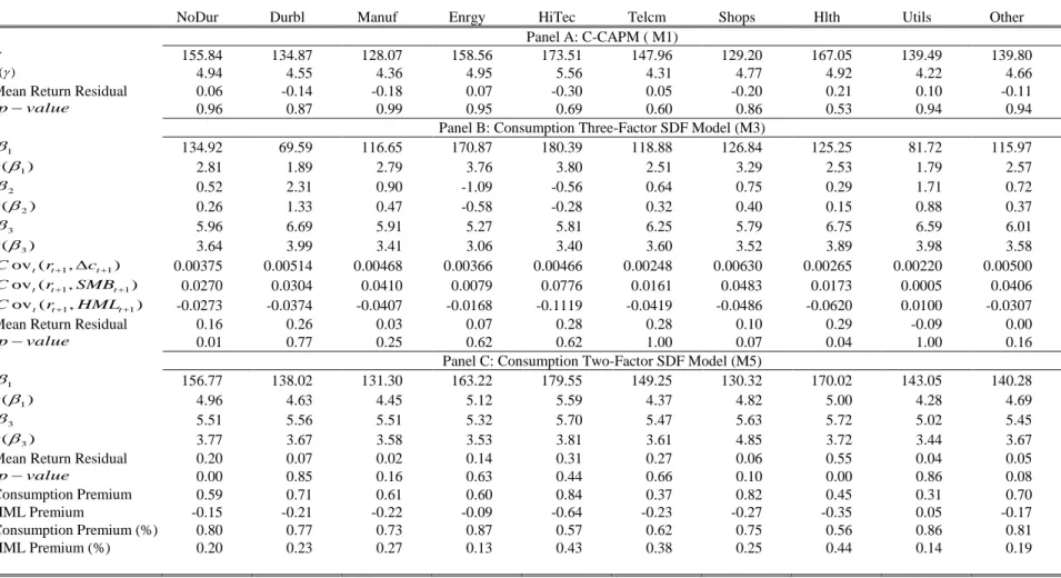
We also examine the behavior of average returns across industry as the performance of different industries is expected to vary across the business cycle. The standard C-CAPM cannot explain the industry returns that have a relatively low level of
book-to-market ratio and small firm size, but including SMB and HML does not improve the fit of these portfolios either. The inability of the consumption three-factor model to price industry returns is consistent with other related studies (Fama and French, 1997; Ferson and Locke, 1998; and Pastor and Stambaugh, 1999). As size and book-to-market ratio for each industry changes over time, it is therefore difficult to measure the share of SMB and HML correctly. In addition, the behavior of the time-varying risk premia for high-technology (HiTec) and utilities (Utils) are similar to those for small growth and big value stocks respectively, as HiTec has a consistently lower book-to-market ratio while Utils has a larger market common equity.
As the choice of HML is empirically motivated, several studies have attempted to establish the connection between HML and more fundamentally determined factors. Fama and French (1995) suggest that the value premium is due to financial distress. Vassalou and Xing (2004) point out that although HML contain default-risk information, HML contains important price information unrelated to default risk. Our results suggest that financial distress and default risk may not be the reason that HML can explain the equity returns as the relation between HML and size indicates that small firms are less risky than big firms. One possible explanation is that HML may be associated with the investment growth prospect of firms. Low book-to-market ratio firms may be expected to have higher rates of growth while, to a lesser extent, small firms may also be expected to behave similarly. Li, Vassalou, and Xing (2006) proposed a sector investment growth model that can explain the cross-section of equity returns, including the small growth portfolio that cannot be priced by most pricing models.
Recent studies attempt to explain the cross-section of equity returns with the modified versions of the standard C-CAPM. By asserting that there are some alternative factors missing from the standard C-CAPM, and taking into account these factors through either conditioning variables (e.g. Lettau and Ludvigson, 2001) or alternative related consumption factors (e.g. Parker and Julliard, 2005; and Yogo, 2006), these modified versions of the standard C-CAPM can explain the cross-section of equity returns as good as (or better than) the Fama and French three-factor model. We take a different approach by using the MGM to directly measure the underlying source of risk premium. This is in contrast to most of the econometric models of equity in the literature that are univariate. Smith, Sorensen, and Wickens (2008) followed this approach and employed the SDF model to generate models involving macroeconomic variables.
In Section I, we discuss the asset pricing theoretical framework. Section II describes the econometric methodology. In Section III, we report the estimates for all portfolio returns. Section IV looks at industry portfolios, and Section V summarizes the findings in this study.
I. Theoretical Framework
A. Stochastic Discount Factor
The SDF is based on a proposition that the price of an asset at the beginning of period
t (Pt) is determined by the expected discounted value of the asset’s payoff in period t+1:
1 1
[ ]
t t t t
where Mt+1 is the stochastic discount factor for period t+1. For equity, the payoff in real terms is Xt+1=Pt+1+Dt+1, where Dt+1 are dividend payments assumed to be made at the start of period t+1. The pricing equation (1) can be written as:
1=E Mt
[
t+1(Xt+1/Pt)]
=E Mt[
t+1Rt+1]
(2) where Rt+1=Xt+1/Pt is the asset’s gross real return. If mt+1=lnMt+1, rt+1 =lnRt+1, and the logarithm of the risk free rate (rtf ) are jointly normally distributed, then the expected excess real return on equity is given by1 1 1 1 1 ( ) ( ) ( , ) 2 f t t t t t t t t E r+ −r + V r+ = −Cov m+ r+ . (3)
The right-hand side is the risk premium and the variance term is the Jensen effect.
The no-arbitrage condition (3) can also be expressed in terms of nominal returns. If
1
t
i+ is the nominal return on equity, f t
i is the nominal risk-free rate, c t
P is the consumer price index, and inflation is given by 1+πt+1 =Ptc+1/Ptc. The pricing equation (1) can be expressed as
1 1 1
1=E Mt t+ (Ptc/Ptc+ )(1+it+). The no-arbitrage condition for nominal returns is:
1 1 1 1 1 1 1 ( ) ( ) ( , ) ( , ) 2 f t t t t t t t t t t t E i+ −i + V i+ = −Cov m+ i+ +Cov π + i+ . (4)
Comparing (4) to (3), the no-arbitrage condition for the nominal return involves one additional term on the right-hand side: the conditional covariance of returns with inflation.
A general linear factor model where z iit( =1,...,n−1) are n−1 factors that are jointly
log normally distributed with equity returns implies the discount factor
1
1 ,
n
t i i i t
m = −
∑
=−α z and the no-arbitrage condition1 0 1 1 , 1 1
( f) ( ) n ( , )
t t t t t i i t i t t
E i+ −i =βV i+ +
∑
= βCov z + i+ (5) =β0V it(t+1)+∑
in=1βifi t, 1+where fi t,+1 are known as common factors. Such models will not necessarily have a general equilibrium interpretation. Different asset pricing models differ mainly due to their stochastic discount factor, zi t,+1, and the restrictions imposed on the coefficients. We consider three pricing models that can be shown to be special cases of Equation (5): 1) C-CAPM with power utility, 2) Fama and French three-factor model, and 3) consumption three-factor model.
B. C-CAPM
The C-CAPM is a general equilibrium model, which implicitly defines the discount factor as
(
)
1 '( 1) / '( )
t t t
M + =β U C+ U C
where Ct is consumption and U C'( t) is utility. For the power utility function,
1
( t) ( t 1) /(1 )
U C = C−γ − −γ with γ =constant coefficient of relative risk aversion (CRRA).
Thus, the SDF becomes Mt 1
(
Ct 1/Ct)
γβ −
+ = + . For nominal return, the relevant no-arbitrage condition can be expressed as
1 1 1 1 1 1 1 ( ) ( ) ( ln , ) ( , ) 2 f t t t t t t t t t t t E i+ −i + V i+ =γCov ∆ C+ i+ +Cov π + i+ , (6)
where ∆lnCt+1 ∆Ct+1/Ct is the growth rate of consumption. The C-CAPM with power utility implies that average excess returns differ due to their conditional covariance with consumption, and the CRRA should be the same across equities.
C. Fama and French Three-Factor Model
Fama and French (1993) extended the CAPM by including, along with the market factor ( m1
t
r+ ), a factor related to size (SMB) and a factor related to book-to-market ratio (HML). SMB is the realization of a capitalization-based factor portfolio that buys small stocks and sells large stocks, holding book-to-market ratio constant. Similarly, HML is the average return on a high book-to-market portfolio minus the average return on a low book-to-market portfolio, holding capitalization constant. The time series averages of SMB and HML can be interpreted as the average risk premia for size and book-to-market ratio. These two factors are therefore a measure of the impact of the underlying features projected onto equity returns.
The Fama and French three-factor model can be shown to be a particular version of the affine multi-factor SDF model, which implies that the expected return must be linearly related to the conditional covariances of its return with rtm+1, SMB, and HML as follows;
1 1 1 1 2 1 1 3 1 1
( f) ( m , ) ( , ) ( , )
t t t t t t t t t t t t
E i+ −i =βCov i+ i+ +β Cov SMB+ i+ +β Cov HML+ i+ .
There is no Jensen effect because log-normality is not assumed. This is an extension to the CAPM where the expected return is defined as:
1 1 1
( f) ( m , )
t t t t t t t
E i+ −i =δCov i+ i+
where δt =E rt( tm+1−rtf) /V rt(tm+1) is the market price of risk, and can be interpreted as the CRRA (Merton (1980)).
Fama and French (1996) argued that the variation in equity returns captured by SMB and HML can be interpreted that asset prices conform to multi-factor models such as the intertemporal CAPM (ICAPM) of Merton (1973) or the arbitrage pricing theory (APT) of Ross (1976), with subsequent support for the ICAPM interpretation given by Liew and Vassalou (2000) and Vassalou (2003). The interpretation of the Fama and French three-factor model as a particular version of the multi-three-factor SDF model (with a general equilibrium derivation) is consistent for the ICAPM only. The ICAPM relates the risk premium to the covariance of returns with wealth and other state variables that reflect investors’ investment opportunities set as well as their payoff at the end period. In contrast, the APT is not in general an SDF model as its coefficient on the risk factor needs not be a conditional covariance.
D. Consumption Three-Factor Model
We extend the standard C-CAPM in much the same way as was done to the CAPM by Fama and French (1993). Without seeking its general equilibrium representation, the consumption three-factor model can be viewed as a particular version of the affine multi-factor SDF model (Equation 5), which has three discount multi-factors (consumption, SMB, and HML). It allows these factors to have unrestricted coefficients for conditional covariances of returns with the factors. The no-arbitrage condition for each asset can be written as
1 1 1 1 1 2 1 1 3 1 1 1 1 1 ( ) ( ) ( , ) ( , ) ( , ) ( , ) 2 f t t t t t t t t t t t t t t t t t
E i+ −i + V i+ =βCov ∆c+ i+ +βCov SMB+ i+ +βCov HML+ i+ +Cov ∆π+ i+ .
As will be shown that SMB has no role in explaining the equity returns in the context of standard CAPM, it is informative to leave out SMB and compare the standard C-CAPM with the consumption two-factor model that contains only consumption and HML. The consumption two-factor model can be written as:
( 1 ) 1 ( 1) 1 ( 1, 1) 3 ( 1, 1) ( 1, 1) 2
f
t t t t t t t t t t t t t t
E i+ −i + V i+ =βCov ∆c+ i+ +βCov HML+ i+ +Cov ∆π+ i+
E. Rational Pricing
As SMB and HML are the time series averages of returns on the mimicking portfolios for the size and value effects, we require that the excess returns on SMB and HML must satisfy the no-arbitrage conditions as well as the portfolios returns. Therefore, this endogenous treatment of SMB and HML eliminates the mispricing hypothesis, implying that the risk premia from SMB and HML arise because they are fundamentally riskier than the risk-free asset. This treatment is in contrast to the approach in Fama and French (1993) where SMB and HML are treated as exogenous variables. In addition, the SDF model implies that the risk premium is represented by the conditional covariances of the returns with the discount factor. This means that the cross-sectional average returns should be solely explained by the cross-sectional variation in their conditional covariances with the factors. Thereby, the coefficients on these conditional covariances should be the same across the cross-section of equity returns. This provides testable restrictions over no-arbitrage conditions.
Essentially, all of these asset pricing models can be represented as restricted versions of the SDF model:
1 0 1 1 1 1 2 1 1 3 1 1 1 1
(sb f) (sb) ( , sb) ( , sb) ( , sb) ( , sb)
t t t t t t t t t t t t t t t t t
E i+ −i =βV i+ +βCov ∆c+ i+ +β Cov SMB+ i+ +βCov HML+ i+ +Cov ∆π+ i+
1 4 1 1 5 1 6 1 1 1 1
( ) ( , ) ( ) ( , ) ( , )
t t t t t t t t t t t t t
E SMB+ =β Cov ∆c+ SMB+ +βV SMB+ +βCov HML+ SMB+ +Cov ∆π+ SMB+
1 7 1 1 8 1 1 9 1 1 1
( ) ( , ) ( , ) ( ) ( , )
t t t t t t t t t t t t t
E HML+ =βCov ∆c+ HML+ +βCov HML+ SMB+ +βV HML+ +Cov ∆π+ HML+
where s = 1, 2,…, 5 and b = 1,2,…, 5 indicate size and book-to-market ratio groups that characteristics portfolios belong to respectively. The numbers are in ascending order of magnitude. For example, the smallest (largest) size group is denoted by s=1(5) while the lowest (highest) book-to-market groups is represented by b=1(5). For the industry portfolios, sb is replaced by the industry name defined by SIC code. The different asset models can be obtained by placing different restrictions onβi.
Table I provides a summary of restrictions on the standard C-CAPM, the consumption three-factor model, and the consumption two-factor model. The standard C-CAPM implies that the CRRA is constant and should be the same across portfolio returns for no arbitrage opportunities in the market (M1). On the other hand, allowing the coefficients of the conditional covariances of returns with consumption to be different generates an unrestricted version of the standard C-CAPM (M2). Similarly, these restrictions of the standard C-CAPM are applied for the other two augmented consumption models (M3-M6).
Table I
Restrictions on the No-Arbitrage Condition
βi is the slope coefficients on the conditional covariances of portfolio returns with consumption growth,
SMB, and HML. Model β0 β1 β2 β3 β4 β5 β6 β7 β8 β9 M1: C-CAPM 1 2 − γ 0 0 γ 1 2 − 0 γ 0 1 2 − M2: Unrestricted C-CAPM 1 2 − β1 0 0 β4 1 2 − 0 β7 0 1 2 − M3: Restricted Consumption Three-Factor Model 1 2 − β1 β2 β3 β1 2 1 2 β − 3 β β1 β2 3 1 2 β − M4: Unrestricted Consumption Three-Factor Model 1 2 − β1 β2 β3 β4 5 1 2 β − 6 β β7 β8 9 1 2 β − M5: Restricted Consumption Two-Factor Model 1 2 − β1 0 β3 β1 0 β3 β1 0 3 1 2 β − M6: Unrestricted Consumption Two-Factor Model 1 2 − β1 0 β3 β4 0 β6 β7 0 9 1 2 β −
II. Econometric Methodology
As in Smith and Wickens (2002), we use the multivariate generalized autoregressive conditional heteroskedasticity in mean model (MGM) to estimate the joint distribution of the excess return on equity with the macroeconomic factors in such a way that satisfies the no-arbitrage condition under the SDF framework. This is achieved by including conditional covariances of the excess equity returns and the discount factors in the mean of the asset pricing equations.
Let xt 1+ =(ri t, 1+ −rtf,SMBt+1,HMLt+1,πt+1,∆ct+1,∆qt+1) ' and contains n variables. Consumption, SMB, HML are included as the discount factors in M1-M6. Industrial production is also included in this vector as an additional macroeconomic variable to improve the estimate of the joint distribution. The MGM model can be written as
(
)
1 1
t+ = +α t + t+1 n+εt+
x Γx λ H 1 ,
εt+1|It ~ N(0,Ht+1),
where, α is a n×1 vector of constant, Γ is a n n× matrix of coefficients in the vector autoregressive (VAR) part, λ is a n n× matrix of coefficients of in-mean component, εt+1 is an n×1 vector of errors, and i= number of equity returns. The error term, εt+1, is conditionally normally distributed with mean zero and the conditional covariance matrix (Ht+1). The first 3 rows of the model are restricted to satisfy the no-arbitrage condition as follows: 1) the first 3 rows of Γ must be zero, 2) the first 3 rows of
λ depends on specification of each asset pricing model defined in Table I, 3) the 4th to 6th rows of λ are all zero, and 4) the first 3 elements of α are zero. The VAR matrix is included to obtain better representation of the error terms, and to examine the relation between SMB, HML, and other macroeconomic variables. A log-likelihood ratio test is used to provide test statistics for the restrictions on the coefficients of conditional covariances with the discount factor implied by the no-arbitrage condition in M1-M6.
The MGM can be expressed as
, 1 , 1 1 1 1 1 2 3 4 5 6 1 2 1 2 3 4 5 6 1 3 1 2 3 4 5 6 1 0 0 0 0 0 0 0 0 0 0 0 0 0 0 0 0 0 0 0 0 0 f f i t t i t t t t t t t t t t t t r r r r SMB SMB HML HML c c q q α γ γ γ γ γ γ π π α φ φ φ φ φ φ α τ τ τ τ τ τ + − + + + + + − − = + ∆ ∆ ∆ ∆ , 1 1 1 1 1 1 1 2 3 4 5 6 1 7 8 9 10 11 12 1 13 14 15 16 17 18 1 1 1 1 0 0 0 0 0 0 0 0 0 0 0 0 0 0 0 0 0 0 i t t t t t t r t SMB t HML t t c t q t π λ λ λ λ λ λ ε λ λ λ λ λ λ ε λ λ λ λ λ λ ε ε ε ε + + + + + + + + + + ∆ + ∆ + + ⋅ + t+1 n t H 1 .
An example of the restrictions on the in-mean coefficient matrix for the consumption three-factor model (M3) is given by
2 3 1 2 3 1 2 3 1 1 1 0 2 1 0 ( ) 1 0 2 1 0 ( ) 1 0 2 0 0 0 0 0 0 0 0 0 0 0 0 0 0 0 0 0 0 β β β β β β β β β − − = − λ .
There are two parameters that affect the conditional variance of SMB and HML in each equation. The first -½ is from the log-normality assumption, and the second, β2 for SMB and β3 for HML, is from the no arbitrage condition.
The MGM model is highly parameterized which can create numerical problems in finding the maximum of the likelihood function due to the likelihood being relatively flat and uninformative. Therefore, to complete the model parameterization for the conditional covariance matrix Ht+1 with the view of restricting the number of coefficient being estimated, the specification of the conditional covariance matrix is chosen to be the vector diagonal model with variance targeting (Ding and Engle, 2001), which can be written as follows,
Ht+1 =H ii - aa - bb0( / / /)+aa/ (ε εt /t)+bb/ Ht
where denotes Hadamard product, H0 is the observed sample covariance matrix, a
and b are n×1 vectors. The number of parameters to be estimated reduces to only 2n, allowing us to focus on estimating the parameters in the in-mean component and the VAR matrix. For instance, estimating the standard C-CAM (M1) involved 34 parameters, while those for the consumption three-factor model (M3) involves 36 parameters respectively as we need to include two more discount factors in the joint distribution.
III. Data
Tables II and III show the monthly data on portfolios returns and macroeconomic variables from 1960.2 to 2004.11 for the US (538 observations). The return on the market portfolio is the value-weighted return on all stocks. The return on a risk-free asset is the one-month Treasury bill rate. There are two datasets of portfolio returns consisting of the 25 value-weighted portfolios formed by the intersections of 5 size and book-to-market quintiles and the 10 industry portfolios defined by the SIC codes. sb is used to defined the 25 portfolios according to their size and book-to-market groups. Portfolio 11 refers to the portfolio in the lowest book-to-market and smallest size quintiles. Real non-durable growth consumption is from the Federal Reserve Bank of St. Louis. CPI inflation and the volume index of industrial production are both from Thomson Reuters Datastream. All of the return variables are obtained from the data library webpage of Kenneth French Real non-durable growth consumption is from the Federal Reserve Bank of St. Louis. CPI inflation and the volume index of industrial production are both from Datastream.
Table II
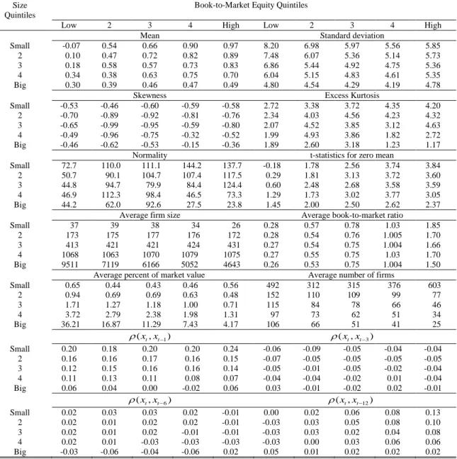
Descriptive Statistics: 25 Size and Book-to-Market Portfolios
The table presents descriptive statistics for the excess returns on the 25 portfolios formed as the intersections of the five size and book-to-market ratio groups. Data and full definition of the returns can be found on http://mba.tuck.dartmouth.edu/pages/faculty/ken.french/data_library.html.The returns are monthly value-weighted from 1960.2 to 2004.11, 538 observations. t-stat is the test statistics for zero mean hypothesis.ρ( xt , x t-i ) represents the autocorrelation coefficients over the time interval i month (s).
Size Quintiles
Book-to-Market Equity Quintiles
Low 2 3 4 High Low 2 3 4 High
Mean Standard deviation
Small -0.07 0.54 0.66 0.90 0.97 8.20 6.98 5.97 5.56 5.85
2 0.10 0.47 0.72 0.82 0.89 7.48 6.07 5.36 5.14 5.73
3 0.18 0.58 0.57 0.73 0.83 6.86 5.44 4.92 4.75 5.36
4 0.34 0.38 0.63 0.75 0.70 6.04 5.15 4.83 4.61 5.35
Big 0.30 0.39 0.46 0.47 0.49 4.80 4.54 4.29 4.19 4.78
Skewness Excess Kurtosis
Small -0.53 -0.46 -0.60 -0.59 -0.58 2.72 3.38 3.72 4.35 4.20
2 -0.70 -0.89 -0.92 -0.81 -0.76 2.34 4.03 4.56 4.23 4.32
3 -0.65 -0.99 -0.95 -0.59 -0.80 2.07 4.52 3.85 3.12 4.63
4 -0.49 -0.96 -0.75 -0.32 -0.52 1.99 4.93 3.86 1.82 2.72
Big -0.46 -0.62 -0.53 -0.15 -0.36 1.89 2.60 3.18 1.23 1.17
Normality t-statistics for zero mean
Small 72.7 110.0 111.1 144.2 137.7 -0.18 1.78 2.56 3.74 3.84
2 50.7 90.1 104.7 107.4 117.5 0.29 1.81 3.13 3.72 3.60
3 44.8 94.7 79.9 84.4 124.4 0.60 2.48 2.68 3.58 3.59
4 46.9 112.3 98.4 46.5 73.3 1.29 1.73 3.02 3.77 3.05
Big 44.2 62.0 92.6 27.5 23.8 1.45 2.00 2.50 2.62 2.37
Average firm size Average book-to-market ratio
Small 37 39 38 34 26 0.28 0.57 0.78 1.03 1.85
2 173 175 177 176 172 0.28 0.54 0.76 1.005 1.70
3 413 421 421 424 431 0.27 0.54 0.75 1.004 1.66
4 1068 1063 1070 1079 1075 0.27 0.55 0.75 1.03 1.70
Big 9511 7119 6166 5052 4643 0.26 0.53 0.75 1.004 1.50
Average percent of market value Average number of firms
Small 0.65 0.44 0.43 0.46 0.56 492 312 315 376 603 2 0.94 0.69 0.69 0.63 0.48 152 110 109 99 77 3 1.71 1.27 1.18 1.00 0.71 115 84 78 66 46 4 3.72 2.79 2.38 1.98 1.31 97 73 62 51 34 Big 36.21 16.87 11.29 7.43 4.17 106 66 51 41 25 1 (x xt, t ) ρ − ρ(x xt, t−3) Small 0.20 0.18 0.20 0.20 0.24 -0.06 -0.09 -0.05 -0.04 -0.04 2 0.16 0.16 0.17 0.16 0.15 -0.07 -0.05 -0.05 -0.05 -0.05 3 0.12 0.15 0.16 0.16 0.14 -0.05 -0.01 -0.05 -0.02 -0.04 4 0.11 0.13 0.11 0.08 0.07 -0.04 -0.04 -0.02 0.01 -0.04 Big 0.06 0.04 0.00 -0.02 0.06 0.03 -0.01 -0.02 0.02 -0.01 6 (x xt, t ) ρ − ρ(x xt, t−12) Small 0.02 0.03 0.03 0.02 -0.01 0.00 0.02 0.06 0.08 0.13 2 0.02 0.01 0.02 0.02 -0.01 -0.03 0.03 0.05 0.08 0.10 3 0.02 0.01 0.02 -0.01 -0.01 -0.03 0.03 0.02 0.04 0.08 4 0.02 0.01 -0.03 -0.03 -0.03 -0.03 0.00 0.03 0.06 0.06 Big -0.03 -0.06 -0.04 -0.06 0.02 0.05 0.01 0.02 0.02 0.02
Table III
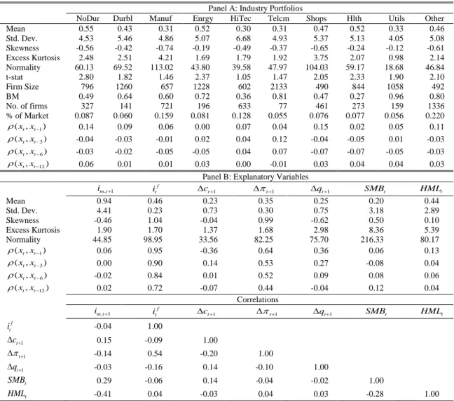
Summary Statistics: 10 Industry Portfolios and Explanatory Variables
The table presents descriptive statistics for the returns on the 10 industry-sorted portfolios and explanatory variables. The returns are monthly value-weighted from 1960.2 to 2004.11, 538 observations. The NYSE, AMEX, and NASDAQ stocks are assigned to an industry portfolio based on its four-digit SIC code. im,t+1
and itf are the returns on the market portfolios and one-month Treasury bill rate respectively. Consumption
growth, inflation, and industrial production growth are represented by ∆ct+1, ∆πt+1, and ∆qt+1 respectively.
Std. Dev is the standard deviation. t-stat is the t-statistic for zero mean hypothesis. t-stat is the test statistics for zero mean hypothesis. ρ( xt , x t-i )represents the autocorrelation coefficients over the time interval i
month(s). BM denotes book-to-market equity ratio. Firm size, book-to-market equity ratio, percent of the market, and number of firms are in average terms. Data and full definition of 10 industries can be found on http://mba.tuck.dartmouth.edu/pages/faculty/ken.french/data_library.html.
Panel A: Industry Portfolios
NoDur Durbl Manuf Enrgy HiTec Telcm Shops Hlth Utils Other
Mean 0.55 0.43 0.31 0.52 0.30 0.31 0.47 0.52 0.33 0.46 Std. Dev. 4.53 5.46 4.86 5.07 6.68 4.93 5.37 5.13 4.05 5.08 Skewness -0.56 -0.42 -0.74 -0.19 -0.49 -0.37 -0.65 -0.24 -0.12 -0.61 Excess Kurtosis 2.48 2.51 4.21 1.69 1.79 1.92 3.75 2.07 0.98 2.14 Normality 60.13 69.52 113.02 43.80 39.58 47.97 104.03 59.17 18.68 46.84 t-stat 2.80 1.82 1.46 2.37 1.05 1.47 2.05 2.33 1.90 2.10 Firm Size 796 1260 657 1228 602 2133 490 844 1058 492 BM 0.49 0.64 0.60 0.72 0.36 0.81 0.47 0.27 0.96 0.80 No. of firms 327 141 721 196 633 77 461 273 159 1336 % of Market 0.087 0.060 0.159 0.081 0.128 0.055 0.076 0.077 0.056 0.220 1 (x xt, t ) ρ − 0.14 0.09 0.06 0.00 0.07 0.04 0.15 0.02 0.05 0.11 3 (x xt, t ) ρ − -0.04 -0.03 -0.01 0.02 0.04 0.12 -0.04 -0.05 0.01 -0.03 6 (x xt, t ) ρ − -0.03 -0.02 -0.05 -0.05 0.04 0.07 -0.07 -0.07 -0.05 -0.03 12 (x xt, t ) ρ − 0.06 0.01 0.01 0.03 0.00 -0.01 0.03 0.04 0.04 0.03
Panel B: Explanatory Variables
, 1 m t i + f t i ∆ct+1 ∆πt+1 ∆qt+1 SMBt HMLt Mean 0.94 0.46 0.23 0.35 0.25 0.20 0.44 Std. Dev. 4.41 0.23 0.73 0.30 0.75 3.18 2.89 Skewness -0.46 1.04 -0.04 0.99 -0.62 0.50 0.10 Excess Kurtosis 1.90 1.70 1.37 1.68 2.98 8.36 5.39 Normality 44.85 98.95 33.56 82.25 75.70 216.33 80.17 1 (x xt, t ) ρ − 0.06 0.95 -0.36 0.64 0.36 0.06 0.13 3 (x xt, t ) ρ − 0.00 0.90 0.14 0.53 0.27 -0.08 0.04 6 (x xt, t ) ρ − -0.02 0.84 0.01 0.52 0.09 0.08 0.06 12 (x xt, t ) ρ − 0.02 0.72 -0.07 0.44 -0.04 0.12 0.04 Correlations , 1 m t i + itf ∆ct+1 ∆πt+1 ∆qt+1 SMBt HMLt f t i -0.04 1.00 1 t c+ ∆ 0.15 -0.09 1.00 1 t π+ ∆ -0.14 0.54 -0.20 1.00 1 t q+ ∆ -0.03 -0.16 0.14 -0.10 1.00 t SMB 0.29 -0.06 0.14 -0.04 -0.02 1.00 t HML -0.41 0.04 -0.03 0.04 0.03 -0.28 1.00
The descriptive statistics for the excess returns of the 25 portfolios in Table II are similar to those in Fama and French (1993) for the period 1963-1991. This indicates a stronger value effect and relatively weak size effect. For the 10 industry portfolios, the telecommunications industry (Telcm) has the highest average book-to-market ratio and largest firm size. The Hi-technology industry (HiTec) has the highest standard deviation and the lowest average excess return. In general, most of the excess returns and macroeconomic variables appear to have negative skewness, excess kurtosis, and non-normality, except the risk-free rate, SMB, HML, and inflation that display positive skewness and show volatility persistent.
IV. Estimates of 25 Size and Book-to-Market Portfolios
A. C-CAPM
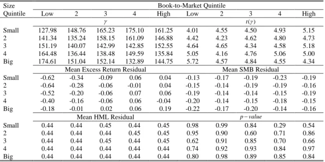
Table IV reports the estimates for M1. The conditional covariances of returns with consumption for all portfolios are highly significant. However, their sizes that range from 127.98 to 174.61 imply implausibly large CRRA, which is a common feature of consumption-based models (Campbell, 2002; Yogo, 2006; Smith, Sorensen, and Wickens, 2008). We do not observe a systemic relation in the consumption coefficients across size or book-to-market ratio. The likelihood ratio statistics support the hypothesis that the consumption coefficients are the same for each portfolio return, SMB, and HML. This result implies that the no-arbitrage condition under the standard C-CAPM is satisfied as the coefficients on the conditional covariances of each portfolio return, SMB, and HML
return, SMB, and HML differs because the cross-sectional variation in their conditional covariances with consumption.
Table IV
Standard C-CAPM (M1): 25 Size and Book-To-Market Portfolios
The table presents the estimates of the standard C-CAPM (M1) for the 25 size and book-to-market portfolios: 1960.2-2004.11, 538 observations. The model is estimated by the multivariate GARCH in mean model. γ and ( )tγ denote the coefficient relative risk aversion and its corresponding t–statistics respectively. The mean residual is computed by subtracting the predicted excess return from their historical value. M1 is tested against M2 using the log-likelihood ratio test. The corresponding p-value is denoted by
p-value.
Size Quintile
Book-to-Market Quintile
Low 2 3 4 High Low 2 3 4 High
γ t( )γ Small 127.98 148.76 165.23 175.10 161.25 4.01 4.55 4.50 4.93 5.15 2 141.34 135.24 158.15 161.09 146.88 4.42 4.23 4.62 4.80 4.73 3 151.19 140.07 142.99 142.85 152.55 4.64 4.65 4.34 4.58 5.18 4 164.48 136.44 138.48 149.59 135.84 5.05 4.16 4.76 5.06 5.00 Big 174.61 151.04 152.14 132.89 144.75 5.72 4.57 4.84 4.55 4.34
Mean Excess Return Residual Mean SMB Residual
Small -0.62 -0.34 -0.09 0.06 0.04 -0.13 -0.17 -0.19 -0.23 -0.19 2 -0.64 -0.28 -0.06 -0.01 0.04 -0.15 -0.14 -0.19 -0.19 -0.16 3 -0.52 -0.20 -0.06 0.07 0.06 -0.19 -0.14 -0.14 -0.15 -0.19 4 -0.40 -0.16 -0.06 0.06 -0.04 -0.20 -0.14 -0.15 -0.18 -0.15 Big -0.18 -0.01 0.02 0.06 0.19 -0.22 -0.17 -0.20 -0.14 -0.16
Mean HML Residual p value−
Small 0.44 0.44 0.45 0.44 0.45 0.98 0.99 0.84 0.29 0.54 2 0.44 0.44 0.44 0.45 0.45 0.95 0.90 0.60 0.71 0.86 3 0.44 0.44 0.45 0.44 0.45 0.62 0.91 0.85 0.70 0.66 4 0.44 0.44 0.44 0.44 0.44 0.74 0.92 0.93 0.84 0.97 Big 0.44 0.44 0.44 0.44 0.44 0.80 0.98 0.89 0.85 0.84
Figure 1(a) presents the cross-sectional fit of M1. If the pricing model fits the data well, the points should all lie on a 45-degree line. M1 can successfully explain the returns on 15 portfolios, which are mostly in the three highest book-to-market quintiles. The differences between predicted and actual excess returns for these 15 portfolios are less than 0.10% per month. However, M1 cannot explain well the returns on the 10 portfolios mostly in the first two booktomarket quintiles. The highest residuals, 0.62% and
-0.64%, are from the two smallest portfolios in the lowest book-to-market quintile respectively.
Figure 1
Cross-Sectional Fit: 25 Size and Book-to-Market Portfolios
The figure plots average actual versus predicted excess returns (% per month) for the 25 size and book-to-market portfolios. The estimated models are (a) Standard C-CAPM, (b) Consumption three-factor model, and (c) Consumption two-factor model. The average excess returns are adjusted for the Jensen effect. The 25 portfolios are defined using two numbers, sb. s = 1,…, 5 and b = 1,…, 5 indicate size and book-to-market groups that portfolios are in respectively. The numbers are in ascending order of magnitude. For example, the smallest (largest) size group is denoted by s = 1 (5) while the lowest (highest) book-to-market groups is represented by b = 1 (5). 0.1 0.3 0.5 0.7 0.9 1.1 0.1 0.3 0.5 0.7 0.9 1.1 Pr edicted R is k Pr emium
Average Excess Return (a) C-CAPM: M1 11 21 31 51 52 42 41 53 54 55 22 33 32 43 12 13 45 3444 23 2435 25 14 15 0.1 0.3 0.5 0.7 0.9 1.1 0.1 0.3 0.5 0.7 0.9 1.1 Pr edicted R is k Pr emium
Average Excess Return (b) Three-Factor SDF Model: M3 11 21 31 51 52 42 41 53 54 55 2233 3243 12 13 45 344423 24 35 25 14 15 0.1 0.3 0.5 0.7 0.9 1.1 0.1 0.3 0.5 0.7 0.9 1.1 Pr edicted R is k Pr emium (c) Two-Factor SDF Model: M5 11 21 31 51 52 42 4153 54 55 2233 3243 12 13 45 344423 24 35 25 14 15
The inability of M1 to price the small growth portfolios (Portfolios 11 and 21) is consistent with other studies (Fama and French, 1993; Lettau and Lugvigson, 2001; Parker and Julliard, 2005; Yogo, 2006) where the pricing models have difficulty in explaining the portfolios in the small size and low book-to-market quintiles (small growth portfolio). This inability may come from limits arbitrage that is due to short-sale constraints for these portfolios. Thus, frictionless equilibrium models, including the C-CAPM, cannot explain the returns on these small growth portfolios (Yogo, 2006). In addition, M1 is also not able to explain the variations on SMB and HML. The average residuals for SMB and HML are -0.17% and 0.44% per month respectively.
B. Consumption Three-Factor Model
Table V reports the estimates of the consumption three-factor model (M3). As in M1, all of the consumption coefficients are significantly different from zero at conventional level, and their magnitudes range from 114.06 to 207.92. The inclusion of SMB and HML as additional risk factors does not affect the way consumption determines asset returns. SMB plays no role in explaining the equity returns as none of its coefficients is significant. On the other hand, HML appears to be able to explain asset returns. All of the coefficients for the conditional covariances of returns with HML are more than three standard errors. The explanatory power of HML is as strong as consumption. These HML coefficients are similar, having an average value of 5.44. Therefore, the differences in HML risk premium across portfolios should come from the differences in their conditional covariances with HML, and, in fact, the likelihood ratio statistics for 18 portfolios suggest that M3 is preferred to M4.
Table V
Consumption Three-Factor Model (M3): 25 Size and Book-to-Market Portfolios
The table presents the estimates of the three-factor SDF model (M3) for the 25 size and book-to-market portfolios: 1960.2-2004.11, 538 observations. The model is estimated by the multivariate GARCH in mean model. β1, β2, and β3 are slope coefficients on consumption, SMB, and HML factors respectively. The
mean residual is computed by subtracting the predicted excess return from their historical value. M3 is tested against M4 using the log-likelihood ratio test. The corresponding p-value denoted by p-value.
Size quintile
Book-to-market equity quintile
Low 2 3 4 High Low 2 3 4 High
1 β t(β1) Small 114.06 149.98 182.42 207.92 171.56 2.62 3.45 3.39 3.81 4.04 2 136.49 134.27 170.65 172.99 152.22 3.25 3.37 3.72 3.91 3.82 3 157.17 141.59 142.31 146.19 158.69 3.52 3.80 3.40 3.62 4.05 4 175.63 136.88 137.89 156.57 129.87 4.19 3.12 3.83 4.10 3.78 Big 187.08 156.45 153.40 127.71 142.82 4.46 3.55 3.73 3.53 2.97 2 β t(β2) Small 0.96 0.06 -0.74 -1.73 -0.55 0.47 0.03 -0.36 -0.80 -0.29 2 0.34 0.10 -0.68 -0.65 -0.19 0.18 0.05 -0.35 -0.33 -0.10 3 -0.56 0.24 0.24 -0.06 -0.28 -0.27 0.13 0.12 -0.03 -0.14 4 -0.81 0.10 0.22 -0.41 0.48 -0.43 0.05 0.12 -0.22 0.27 Big -0.69 -0.18 -0.01 0.60 0.34 -0.37 -0.09 -0.01 0.33 0.17 3 β t(β3) Small 5.73 5.46 5.30 4.89 5.15 3.74 3.54 3.42 3.11 3.29 2 5.64 5.48 5.46 5.42 5.38 3.58 3.49 3.53 3.43 3.35 3 5.15 5.95 5.59 5.35 5.44 3.22 3.93 3.61 3.42 3.47 4 5.39 5.75 5.71 5.12 5.42 3.50 3.66 3.68 3.30 3.47 Big 5.45 5.56 5.37 5.41 5.40 3.57 3.58 3.38 3.43 3.43
Mean excess return residual Mean SMB residual
Small -0.06 0.05 0.18 0.26 0.17 -0.04 -0.04 -0.03 -0.03 -0.04 2 -0.01 0.05 0.14 0.11 0.12 -0.03 -0.01 -0.03 -0.02 -0.02 3 0.08 0.07 0.07 0.11 0.07 -0.03 -0.02 -0.03 -0.03 -0.04 4 0.14 0.08 0.06 0.09 -0.02 -0.02 -0.01 -0.03 -0.04 -0.04 Big 0.20 0.18 0.14 0.05 0.13 -0.05 -0.03 -0.07 -0.05 -0.06
Mean HML residual p value−
Small 0.01 0.01 0.01 0.01 0.02 0.86 1.00 0.21 0.07 0.51 2 0.00 0.00 -0.01 0.00 0.01 0.88 0.63 0.28 0.08 0.53 3 0.01 -0.03 0.00 0.01 0.00 0.99 0.39 0.05 0.17 0.13 4 -0.01 -0.01 -0.01 0.02 0.02 0.57 0.22 0.12 0.05 0.02 Big 0.00 -0.01 0.01 0.02 0.02 0.09 0.07 0.41 0.18 0.51
Figure 1(b) shows the cross-sectional fit of M3 for the 25 portfolios. Most portfolios appear to earn average excess returns higher than M3 predicts. Although, the largest residual in M3 (0.26% per month) is much lower than in M1 (0.64%), M3 explains only the returns on 11 portfolios (8 portfolios are in the first two lowest book-to-market quintiles) better than M1. These 11 portfolios also include the two small growth
portfolios (Portfolios 11 and 12) that previously have the largest residuals in M1. The average residuals for these two portfolios in M3 are only -0.06% and -0.01% per month.
On the other hand, M1 explains the returns on 13 portfolios better than M3 with 9 portfolios having the average residual smaller than 0.07% (in absolute term) per month. Apart from portfolios with a low book-to-market ratio, M1 appears to do a good job in explaining the equity returns. Including SMB and HML improves mainly the cross-sectional fit of the low book-to-market portfolios. However, M3 can capture the variation in SMB and HML. The biggest SMB residual (-0.07% per month) in M3 is lower than that in M1 (-0.23% per month). For HML, the biggest HML residual is -0.03 % per month, which is significantly smaller than 0.44%-0.45% per month in M1. The ability of M3 to price SMB and HML is consistent with Brennan, Wang, and Xia (2004) where they propose an ICAPM with time-varying investment opportunities that explains well the returns on SMB and HML.
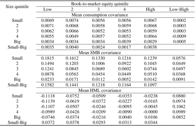
Table VI shows the conditional covariances of the 25 portfolio returns with consumption, SMB, and HML. The consumption covariances decline as size increases while little variation is observed across book-to-market ratio. On the other hand, we observe the systemic movement in the covariances of SMB and HML. All returns positively co-move with SMB. Small firms have higher SMB covariances than large firms, but the spreads in the SMB covariances across size decrease as book-to-market ratio increases. The differences in SMB covariances between the smallest and biggest size quintiles in the lowest to highest book-to-market quintiles are 0.1582, 0.1441, 0.1218, 0.1164, and 0.1097 respectively.
Table VI
Average Covariances: 25 Size and Book-to-Market Portfolios
The table presents the average covariances of the returns on the 25 size and book-to-market portfolios with consumption, SMB, and HML from the estimation of the consumption three-factor model. The process of the conditional covariances is assumed to follow the multivariate GARCH in mean model.
Size quintile Book-to-market equity quintile
Low 2 3 4 High Low-High
Mean consumption covariance
Small 0.0069 0.0074 0.0056 0.0056 0.0067 0.0002 2 0.0071 0.0068 0.0058 0.0059 0.0068 0.0003 3 0.0062 0.0066 0.0052 0.0053 0.0059 0.0003 4 0.0055 0.0049 0.0057 0.0052 0.0064 -0.0009 Big 0.0034 0.0034 0.0034 0.0039 0.0029 0.0005 Small-Big 0.0035 0.0040 0.0024 0.0017 0.0038 Mean SMB covariance Small 0.1815 0.1612 0.1330 0.1216 0.1239 0.0576 2 0.1494 0.1203 0.1006 0.0922 0.1045 0.0449 3 0.1241 0.0845 0.0689 0.0602 0.0744 0.0497 4 0.0878 0.0563 0.0454 0.0449 0.0510 0.0368 Big 0.0233 0.0171 0.0112 0.0052 0.0142 0.0091 Small-Big 0.1582 0.1441 0.1218 0.1164 0.1097 Mean HML covariance Small -0.1118 -0.0752 -0.0509 -0.0353 -0.0238 0.0880 2 -0.1139 -0.0619 -0.0372 -0.0227 -0.0165 0.0974 3 -0.1107 -0.0507 -0.0246 -0.0095 -0.0045 0.1062 4 -0.0989 -0.0426 -0.0209 -0.0090 -0.0000 0.0989 Big -0.0746 -0.0374 -0.0216 0.0040 0.0106 0.0852 Small-Big 0.0372 0.0378 0.0293 0.0313 0.0344
Moreover, SMB seems to be related to market ratio as well. Low book-to-market portfolios co-move with SMB more than high book-to-book-to-market portfolios. However, this relation is not as strong as the co-movement of SMB across size. The differences between SMB covariances for the lowest and highest book-to-market quintiles in the smallest to biggest size quintiles are 0.0576, 0.0449, 0.0497, 0.0368, and 0.0091 respectively. The dispersion of SMB covariance across book-to-market ratio decreases as size increases. The examination of SMB covariance shows that SMB is associated with size and, to a lesser extent, book-to-market ratio. There seems to be a
(book-to-market ratio) tend to be lower as book-to-market ratio (size) increases. The small growth portfolio (Portfolio 11) has the largest SMB covariance (0.1815) because it is in the smallest size quintiles as well as in the lowest book-to-market quintiles.
Most portfolios seem to negatively co-move with HML, with the exception of big value portfolios (large portfolios with high book-to-market ratio: Portfolios 54 and 55). Low to-market portfolios have higher negative HML covariances than high book-to-market portfolios. HML appears to be associated with size as well, but not as strong as HML with book-to-market ratio. The differences between HML covariances for the smallest and biggest size from the lowest to highest book-to-market quintiles (0.0293-0.0378) are lower than half of the dispersion of HML covariances across book-to-market ratio (0.0852-0.1062). Unlike the spreads of SMB covariances, the differences between HML covariances across to-market ratio and size are similar across size and book-to-market ratio respectively. The systemic cross-relation of the 25 portfolio returns, SMB and HML suggest that sorting portfolios based on both size and book-to-market ratio provides a better way to distinguish the cross-section of equity returns.
A time-varying comparison between the small growth portfolio (Portfolio 11) and big value portfolio (Portfolio 55) is given in Figure 2. The volatilities of these two risk premia mainly come from consumption with more volatility for the small growth portfolio. We observe a contrast movement during the dotcom bubble burst that occurs between 2000 and 2002. The risk premium for the small growth portfolio decreases sharply while the risk premium for the big value portfolio increases. The consumption covariance for the big value portfolios seems to be unaffected during this period while
that for the small growth portfolio turns sharply negative. The SMB covariance for the big value portfolio co-varies little while the small growth co-moves more with SMB. Moreover, the SMB covariance for the small growth portfolio increases significantly during the 2000-2002 periods while that for the big value portfolio turns negative.
Like SMB covariance, there is little co-movement between the big value portfolio and HML while the small growth portfolio significantly and negatively co-moves with HML. We observe the opposite movement with HML covariances for these two portfolios from 2000 to 2002. Like consumption covariance, the HML covariance for the small growth portfolio falls sharply while that for the big value portfolio increases slightly. The decrease in consumption and HML covariances during this period also occurs for other 10 portfolios in the two lowest book-to-market quintiles. On the other hand, the HML covariance for 6 portfolios in the two highest book-to-market quintiles and the three biggest size quintiles rise, indicating that these big value stocks become riskier, so investors require extra premia to hold these portfolios.
Figure 2
Small Growth and Big Value Portfolios
The figure compares time-varying risk premia and conditional covariances of the returns with the factors between the small growth (portfolio 11) and big value (portfolio 55) portfolios from the consumption three-factor model (M3). The figures are (a) time-varying risk premia, (b) conditional covariances of the returns with consumption, (c) conditional covariances of the returns with SMB, and (d) conditional covariances of the returns with HML. The sample period is 1960:2-2004:11. Shaded areas are recessions as defined by NBER.
1960 1965 1970 1975 1980 1985 1990 1995 2000 2005 -4 -3 -2 -1 0 1 2 3 4
Predicted Risk Premium
Year
(a) Time Varying Risk Premia for Small Growth and Big Value Portfolios Small Growth Big Value 1960 1965 1970 1975 1980 1985 1990 1995 2000 2005 -0.03 -0.02 -0.01 0.00 0.01 0.02 0.03 Conditional Covariance Year
(b) Conditional Covairances with Consumption Small Growth Big Value 1960 1965 1970 1975 1980 1985 1990 1995 2000 2005 -0.7 -0.5 -0.3 -0.1 0.1 0.3 0.5 0.7 Conditional Covariance
(c) Conditional Covairances with SMB Small Growth Big Value 1960 1965 1970 1975 1980 1985 1990 1995 2000 2005 -0.6 -0.4 -0.2 0.0 0.2 0.4 0.6 Conditional Covariance
(d) Conditional Covairances with HML Small Growth
Table VII
Consumption Two-Factor Model (M5): 25 Size and Book-to-Market Portfolios
The table presents the estimates of the consumption two-factor model (M5) for the 25 size and book-to-market portfolios: 1960.2-2004.11, 538 observations. The model is estimated by the multivariate GARCH in mean model.β1 and β3 are slope coefficients on consumption and HML factors respectively. The mean
residual is computed by subtracting the predicted excess return from their historical value. M5 is tested against M6 using the log-likelihood ratio test. The corresponding p-value is denoted by p-value.
Size quintile
Book-to-market equity quintile
Low 2 3 4 High Low 2 3 4 High
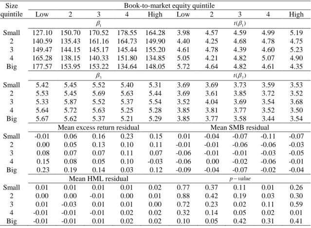
1 β t(β1) Small 127.10 150.70 170.52 178.55 164.28 3.98 4.57 4.59 4.99 5.19 2 140.59 135.43 161.16 164.73 149.90 4.40 4.25 4.68 4.78 4.75 3 149.47 144.15 145.17 145.44 155.20 4.61 4.78 4.39 4.60 5.23 4 165.28 138.15 140.33 151.80 134.85 5.05 4.21 4.82 5.07 4.90 Big 177.57 153.95 153.22 134.64 148.05 5.72 4.64 4.82 4.61 4.35 3 β t(β3) Small 5.42 5.45 5.52 5.40 5.31 3.69 3.69 3.73 3.59 3.53 2 5.53 5.45 5.69 5.63 5.44 3.69 3.61 3.85 3.72 3.52 3 5.33 5.87 5.52 5.37 5.54 3.52 4.04 3.69 3.54 3.68 4 5.64 5.72 5.63 5.25 5.28 3.85 3.81 3.77 3.52 3.50 Big 5.67 5.62 5.37 5.21 5.29 3.85 3.77 3.58 3.44 3.54
Mean excess return residual Mean SMB residual
Small -0.01 0.06 0.16 0.23 0.15 0.01 -0.04 -0.07 -0.11 -0.07 2 0.00 0.05 0.13 0.10 0.11 -0.01 -0.01 -0.06 -0.06 -0.03 3 0.08 0.07 0.07 0.11 0.07 -0.06 -0.01 -0.01 -0.03 -0.05 4 0.15 0.08 0.05 0.10 -0.03 -0.06 0.00 -0.02 -0.06 -0.01 Big 0.23 0.19 0.14 0.03 0.12 -0.09 -0.04 -0.07 -0.02 -0.04
Mean HML residual p value−
Small 0.01 0.01 0.01 0.01 0.02 0.77 0.37 0.11 0.01 0.26 2 0.00 0.00 -0.01 0.00 0.01 0.88 0.42 0.19 0.03 0.30 3 0.01 -0.03 0.01 0.01 0.00 0.72 0.23 0.02 0.11 0.59 4 -0.01 -0.01 -0.01 0.02 0.02 0.32 0.14 0.05 0.02 0.01 Big -0.01 -0.01 0.01 0.02 0.02 0.10 0.05 0.42 0.31 0.41
C. Consumption Two-Factor Model
As SMB is never significant, we further investigate the relation between consumption and HML by comparing M1 with M5. Table VII shows that the consumption and HML coefficients in M5 appear to be similar to those in M3 with a slightly adjustment in the case of consumption, but the significance levels of consumption increase while those for HML are unchanged. The information about equity returns in SMB seems to be more
prices 6 portfolios worse than M5. In addition, M5 can explain the return on HML and SMB well with slightly lower explanatory power for SMB. HML helps explain SMB by reducing the predicted risk premium by consumption.
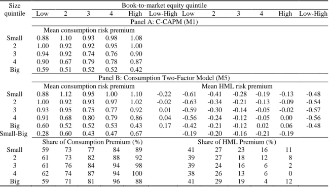
Table VIII shows the contributions to risk premia from consumption and HML in M1 and M5. Including HML as an additional factor does not affect the way consumption generates risk premia since the consumption premia for the 25 portfolios are similar in both models. There seems to be a negative relation in the consumption and size, but no variation in the consumption premia across book-to-market ratio. As most of the HML premia are negative with the exception of two big value portfolios (Portfolios 54 and 55), the effect of HML is to reduce the amount of risk premia generated by consumption. The amount of reduction of risk premium depends on book-to-market ratio and, to a lesser extent, size quintiles the portfolios are in. This is indicated by the co-movement between portfolio returns and HML in Table VI.
Low book-to-market portfolios have a smaller risk premium because they have higher negative covariances with HML. This indicates that low book-to-market portfolios are less risky, and coincides with the value effect. Consistent with Fama and French (2005), the value premia for small and big portfolios are similar, ranging between 0.48% and 0.57% per month. HML is related to size as well, but the relation between HML and size contradicts the size effect. Small firms appear to vary more negatively with HML than big portfolios and earn more negative HML premium. This indicates that small portfolios are less risky and contradicts the prediction of the size effect. The spreads between small and big portfolios across book-to-market quintiles are similar, ranging from 0.16% to
0.21% per month, and are less than half of the value premia as indicated by the spread in the HML covariances.
Table VIII
Contributions to Risk Premia
The table shows the contributions to the risk premia from the consumption and HML factors. The C-CAPM (M1) has only one source generated risk premia while the consumption two-factor model (M5) has two factors determined risk premia. Each contribution is calculated by multiplying the average conditional covariances of the returns with the factors with their respective coefficients estimated by the multivariate GARCH in mean model. The sample is from 1960.2 to 2004.11.
Size quintile
Book-to-market equity quintile
Low 2 3 4 High Low-High Low 2 3 4 High Low-High Panel A: C-CAPM (M1)
Mean consumption risk premium Small 0.88 1.10 0.93 0.98 1.08
2 1.00 0.92 0.92 0.95 1.00 3 0.94 0.92 0.74 0.76 0.90 4 0.90 0.67 0.79 0.78 0.87 Big 0.59 0.51 0.52 0.52 0.42
Panel B: Consumption Two-Factor Model (M5)
Mean consumption risk premium Mean HML risk premium
Small 0.88 1.12 0.95 1.00 1.10 -0.22 -0.61 -0.41 -0.28 -0.19 -0.13 -0.48 2 1.00 0.92 0.93 0.97 1.02 -0.02 -0.63 -0.34 -0.21 -0.13 -0.09 -0.54 3 0.93 0.95 0.75 0.77 0.92 0.01 -0.59 -0.30 -0.14 -0.05 -0.02 -0.57 4 0.91 0.68 0.80 0.79 0.86 0.04 -0.56 -0.24 -0.12 -0.05 0.00 -0.56 Big 0.60 0.52 0.52 0.53 0.43 0.17 -0.42 -0.21 -0.12 0.02 0.06 -0.48 Small-Big 0.28 0.60 0.43 0.47 0.67 -0.19 -0.20 -0.16 -0.21 -0.19
Share of Consumption Premium (%) Share of HML Premium (%) Small 59 73 77 84 89 41 27 23 16 11
2 61 73 82 88 92 39 27 18 12 8 3 61 76 84 94 98 39 24 16 6 2 4 62 74 87 94 100 38 26 13 6 0 Big 59 71 81 96 88 41 29 19 4 12
Portfolios in the lowest book-to-market quintiles are heavily dependent on HML, where about 40% of their total risk premia comes from HML while portfolios in the two highest book-to-market quintiles have HML shares of risk premia less than 20%. There is a negative relation between the HML share of risk premium and book-to-market ratio. The differences in HML shares of risk premium between the lowest and highest book-to-market portfolios are about 29%-38% of total risk premium. On the other hand, the shares of HML premia across size appear to be similar, except that for the fourth highest
book-and size is matched by the movement of HML across size, resulting in constant shares of both consumption and HML premia across size.
As the choice of HML is empirically motivated, several studies have attempted to establish the connection between HML and more fundamentally determined factors. Fama and French (1995) suggested that the value premium was due to financial distress. Low book-to-market ratio is typical of firms with high returns on capital, while high book-to-market ratio is typical of firms that are relatively distressed. Size is also related to earnings. Controlling for book-to-market ratio, small stocks tend to have lower earnings on book equity. Vassalou and Xing (2004) pointed out that, even though HML contain default-risk information, HML contains important price information unrelated to default risk.
Our results suggest that financial distress and default risk may not be the reason that HML can explain the equity returns as the relation between HML premium and size indicates that small firms are less risky than big firms. Even though the size effect arisen from earning properties and captured by SMB in literature or by consumption in this study could possibly dominate the risk premium generated by HML across size, a possible explanation needs to explain why HML predicts that small stocks are less risky than big stocks. One possible explanation is that HML may be associated with investment growth prospects of firms. Low book-to-market ratio firms may be expected to have higher rates of growth while, to a lesser extent, small firms may also be expected to behave similarly. Li, Vassalou, and Xing (2006) proposed a sector investment growth model that can explain the cross-section of equity returns, including the return on the
Figure 3 plots the time-varying contribution to risk premia in M5 for the small growth and big value portfolios. The volatility of the risk premia for both portfolios appears to be mainly driven by consumption premia, with the small growth portfolios having more volatility throughout the sample period. HML always generates negative risk premium for the small growth portfolios. It becomes relatively more important after 1980 as the risk premium for the small growth portfolio is significantly lower than before. Both consumption and HML predict a large fall on the risk premium for the small growth portfolio at the beginning of 2000, but the fall in HML premium is more persistent. Consumption resumes to be working normally in 2001, but the fall in HML premium lasts until 2002.
Figure 3
Contributions to Risk Premia: Small Growth and Big Value
The figure presents the contributions to the risk premia for the small growth (Portfolio 11) and big value (Portfolio 55) portfolios from the two-factor SDF model (M5). The sample period is 1960:2-2004:11. Shaded areas are recessions as defined by NBER.
-5 -4 -3 -2 -1 0 1 2 3 4 5 P re di ct ed Ri sk P re m ium
(a) Small Growth Portfolio
Total Premium Consumption Premium HML Premium
For the big value portfolio, consumption is the only risk factor that significantly affects the behavior of its risk premium. HML premium is close to zero for most of the sample period. A rise in the HML premium for the big value portfolios in 2000 is also associated with the rise in consumption premium, resulting in a sharply increase in total risk premium and indicating that the big value becomes riskier. The dotcom bubble burst in 2000 affects the way consumption and HML generated risk premia for both small growth and big value portfolios in a similar nature with more movement on the HML premium.
D. Constant term
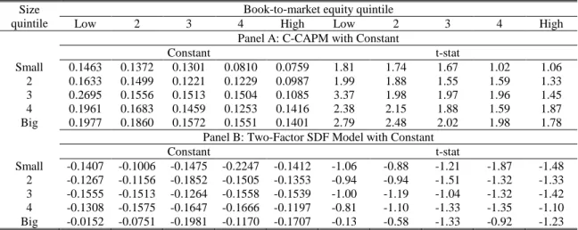
We further compare M1 and M5 by adding a constant term to measure variation in excess returns that was left unexplained in each model. Table IX shows that the magnitudes of the constant terms in both models are similar, but their signs are different.
1960 1965 1970 1975 1980 1985 1990 1995 2000 2005 -3 -2 -1 0 1 2 3 P re di ct ed Ri sk P re m ium Year
(b) Big Value Portfolio
Total Premium Consumption Premium HML Premium
have a negative sign, indicating that the predicted risk premium in M5 is higher than the actual excess returns. The constant terms in M1 for 19 portfolios are significant at 10% confidence level while only 1 portfolio (Portfolio 14) is in M5. As a result, M5 seems to contain more price information about the 25 portfolios returns than M1. This magnitude of the constant terms in the both M1 and M5 is smaller than those in Fama and French (1993). They show that the constant terms for the Fama and French three-factor model ranges from 0.00% to 0.34% (in absolute term) and has 3 portfolios (Portfolios 11, 51, and 42) that have t-statistics more than 2 time standard errors.
Table IX Constant Terms
The table presents the estimates of the constant terms that are included in the estimations of the standard C-CAPM (M1) and the consumption two-factor models (M5) for the 25 size and book-to-market portfolios: 1960.2-2004.11, 538 observations. Both models are estimated by the multivariate GARCH in mean model. t-stat denotes the t–statistics for the constant term.
Size quintile
Book-to-market equity quintile
Low 2 3 4 High Low 2 3 4 High Panel A: C-CAPM with Constant
Constant t-stat Small 0.1463 0.1372 0.1301 0.0810 0.0759 1.81 1.74 1.67 1.02 1.06 2 0.1633 0.1499 0.1221 0.1229 0.0987 1.99 1.88 1.55 1.59 1.33 3 0.2695 0.1556 0.1513 0.1504 0.1085 3.37 1.98 1.97 1.96 1.45 4 0.1961 0.1683 0.1459 0.1253 0.1416 2.38 2.15 1.88 1.59 1.87 Big 0.1977 0.1860 0.1572 0.1551 0.1401 2.79 2.48 2.02 1.98 1.78
Panel B: Two-Factor SDF Model with Constant
Constant t-stat Small -0.1407 -0.1006 -0.1475 -0.2247 -0.1412 -1.06 -0.88 -1.21 -1.87 -1.48 2 -0.1267 -0.1156 -0.1852 -0.1505 -0.1353 -0.94 -0.94 -1.51 -1.32 -1.33 3 -0.1555 -0.1513 -0.1264 -0.1558 -0.1539 -1.00 -1.19 -1.04 -1.32 -1.42 4 -0.1308 -0.1575 -0.1647 -0.1666 -0.1197 -0.81 -1.10 -1.33 -1.35 -1.10 Big -0.0152 -0.0751 -0.1981 -0.1170 -0.1707 -0.13 -0.58 -1.33 -0.92 -1.23
Table X shows the estimates of the VAR matrix for the small growth portfolio in M5 before and after the inclusion of SMB and HML in the VAR matrix (Restricted and Full VAR matrices respectively). The restricted VAR puts zero restrictions on the coefficients