CONFIDENCE INTERVALS (CI) FOR CONCENTRATION
PARAMETER IN VON MISES DISTRIBUTION AND
ANALYSIS OF MISSING VALUES FOR CIRCULAR DATA
SITI FATIMAH BINTI HASSAN
INSTITUTE OF GRADUATE STUDIES
UNIVERSITY OF MALAYA
KUALA LUMPUR
CONFIDENCE INTERVALS (CI) FOR
CONCENTRATION PARAMETER IN VON MISES
DISTRIBUTION AND ANALYSIS OF MISSING VALUES
FOR CIRCULAR DATA
SITI FATIMAH BINTI HASSAN
THESIS SUBMITTED IN FULFILMENT OF THE
REQUIREMENTS FOR THE DEGREE OF DOCTOR OF
PHILOSOPHY
INSTITUTE OF GRADUATE STUDIES
UNIVERSITY OF MALAYA
KUALA LUMPUR
ii UNIVERSITY OF MALAYA
ORIGINAL LITERARY WORK DECLARATION
Name of Candidate: SITI FATIMAH BT HASSAN (I.C No: 841009135224) Registration/Matric No: HHC 100006
Name of Degree: DOCTOR OF PHILOSOPHY
Title of Project Paper/Research Report/Dissertation/Thesis (“this Work”):
CONFIDENCE INTERVALS (CI) FOR CONCENTRATION PARAMETER IN VON MISES DISTRIBUTION AND ANALYSIS OF MISSING VALUES FOR CIRCULAR DATA
Field of Study: STATISTICS
I do solemnly and sincerely declare that: (1) I am the sole author/writer of this Work; (2) This Work is original;
(3) Any use of any work in which copyright exists was done by way of fair dealing and for permitted purposes and any excerpt or extract from, or reference to or reproduction of any copyright work has been disclosed expressly and sufficiently and the title of the Work and its authorship have been acknowledged in this Work;
(4) I do not have any actual knowledge nor do I ought reasonably to know that the making of this work constitutes an infringement of any copyright work; (5) I hereby assign all and every rights in the copyright to this Work to the
University of Malaya (“UM”), who henceforth shall be owner of the copyright in this Work and that any reproduction or use in any form or by any means whatsoever is prohibited without the written consent of UM having been first had and obtained;
(6) I am fully aware that if in the course of making this Work I have infringed any copyright whether intentionally or otherwise, I may be subject to legal action or any other action as may be determined by UM.
Candidate’s Signature Date: Subscribed and solemnly declared before,
Witness’s Signature Date: Name: ASSOC. PROF. DR YONG ZULINA ZUBAIRI
iii
ABSTRACT
This study is on circular statistics that is also known as directional statistics. Directional statistics is a branch of statistics which deal with the data in angle form in which the method of analysis is different from linear data. For example, the distribution analogues to the normal distribution in linear data is known as circular normal distribution. This study comprises of four parts. The first part of the study focuses on the efficient approximation for the concentration parameter in von Mises distribution. Here, a new method of approximating the concentration parameter is proposed, and the performance of the proposed method is studied via simulation study.
The second part of the study is on the confidence intervals (CI) for the concentration parameter in von Mises distribution. Several methods in constructing the CI for the concentration parameter are proposed including CI based on circular population, CI based on the asymptotic distribution of ˆ, CI based on the distribution of
𝜃̅ and 𝑅̅ and also CI based on bootstrap-t method. All proposed methods are validated via simulation study and the performance indicator such as an expected length and its coverage probability are evaluated.
The third part of the study is on the derivation of the circular distance for circular data. From this derivation, we construct the CI for the concentration parameter. Three different methods will be considered in proposing the new CI including mean, median and percentile. The simulation studies carried out to assess the performance of each proposed method.
The final part of this study is an analysis of missing values for circular variables. Missing values is a common problem that occurs in data collection. By ignoring the
iv existence of missing values, leads to the biasness and lack of efficiency of a statistics. In this study, three imputation methods are considered namely expectation-maximization (EM) algorithm and data augmentation (DA) algorithm. All proposed methods are compared to the conventional methods. The analyses are conducted by doing the simulation studies by varying the value of the concentration parameter. All the proposed methods from this study are illustrated using the real data consisting of data in angle form found in the literature.
v
ABSTRAK
Kajian ini adalah mengenai statistik membulat atau lebih dikenali dengan statistik berarah. Statistik berarah adalah suatu cabang bidang yang menggunakan data dalam ukuran sudut dan dengan itu kita memerlukan kaedah yang berlainan dalam menjalankan analisis data tersebut. Kajian ini terbahagi kepada empat bahagian utama. Dalam kajian ini, taburan von Mises akan digunakan sebagai taburan utama dalam melakukan perbincangan kajian. Taburan von Mises juga dikenali sebagai taburan normal membulat dan ia merupakan taburan yang menyerupai taburan normal seperti yang biasa digunakan dalam statistik linear. Bahagian pertama akan memberi focus kepada penganggaran untuk parameter menumpu dalan taburan von Mises. Dalam bahagian ini, kaedah penganggaran terbaru untuk parameter menumpu akan dicadangkan dan diikuti dengan kajian simulasi bagi menilai ketepatan prosedur yang telah dicadangkan.
Bahagian kedua akan membincangkan tentang selang keyakinan (SK) untuk parameter menumpu bagi taburan von Mises. Beberapa kaedah untuk menghasilkan selang keyakinan (SK) akan dicadangkan termasuk SK berdasarkan populasi membulat, SK berdasarkan taburan asimptotik ˆ matrix maklumat Fisher, SK berdasarkan taburan
𝜃̅ dan 𝑅̅ dan SK berdasarkan kaedah bootstrap-t. Semua kaedah yang telah dicadangkan akan disahkan melalui kajian simulasi dan penilaian bagi saiz selang dan kebarangkalian menumpu akan dinilai.
Bahagian ketiga kajian adalah untuk menghasilkn jarak membulat bagi data membulat. Berdasarkan penghasilan ini, didapati kita juga berjaya untuk menghasilkan SK bagi parameter menumpu.Tiga kaedah yang berbeza akan diperkenalkan untuk
vi menghasilkan SK termasuk min, median dan persentil. Kajian simulasi akan dilakukan bagi menilai ketepatan kaedah yang telah dicadangkan.
Bahagian terakhir dalam kajian ini adalah analisis data lenyap bagi pemboleh ubah membulat. Data lenyap merupakan suatu permasalahan biasa dalam pegumpulan data. Dengan hanya mengabaikan kewujudan data yang lenyap atau hilang akan membawa kepada bias dan menyebabkan ia menjadi kurang signifikan secara statistik. Dalam kajian ini, tiga kaedah imputasi akan dicadangkan termasuk ‘expectation maximization’ (EM) dan ‘data augmentation’ (DA). Semua kaedah yang dicadangkan akan dibandingkan dengan kaedah konvensional yang biasa digunakan. Untuk menentukan kaedah terbaik, analisis dibuat melalui kajian simulasi dengan mempelbagaikan nilai parameter menumpu. Akhir sekali, semua kaedah yang telah dicadangkan akan diilustrasi dengan menggunakan data sebenar dalam bentuk sudut yang diperolehi melalui kajian kesusasteraan.
vii
ACKNOWLEDGEMENTS
Alhamdulillah, praise to Allah because I have successfully completed this research. I would like to express my sincere appreciation to my supervisors Prof. Madya Dr. Yong Zulina Zubairi and Prof. Dr. Abdul Ghapor Hussin for their good supervisions, continuous support and encouraging advices throughout the process in completing this research. Thank you very much for being very helpful and supportive.
A special thanks to my parents and husband for being very supportive and understanding throughout the process of completing this research. Without their love and support, it could be very tough journey for me to complete this thesis. Thank you for being there with me all the time.
I deeply thank all my colleague and my dearest friends who always being very supportive and helpful. Thank you for the motivation and advices throughout the completion of my study and thesis. We have shared the moment ups and downs together in the journey of completing this study. Without all the positive vibes from everyone of them, it might be very hard to endure some difficult times through this journey.
Lastly, I would like to thank all visiting lectures that gave comments and help me to improve my research. And, not forgotten, I also would like to thank the University of Malaya and Ministry of Education for providing the scholarship for my study.
viii
TABLE OF CONTENTS
ABSTRACT iii
ABSTRAK v
ACKNOWLEDGEMENTS vii
TABLE OF CONTENTS viii
LIST OF FIGURES xii
LIST OF TABLES xiii
LIST OF APPENDICES xvi
CHAPTER 1: INTRODUCTION
1.1 Background 1
1.2 Problem Statement 5
1.3 Limitation of the Study 6
1.4 Objective 6
CHAPTER 2: LITERATURE REVIEW
2.1 Introduction 7 2.2 Circular Statistics 7 2.2.1 Numerical Statistics 8 2.2.2 Graphical representation 13 2.3 Circular Distribution 14 2.3.1 Uniform Distribution 15
2.3.2 Von Mises Distribution 15
2.3.3 Wrapped Normal Distribution 17
2.3.4 Wrapped Cauchy Distribution 17
2.4 Confidence Intervals 18
2.4.1 Bootstrap Method 19
ix
2.5 Missing Values 27
2.5.1 Traditional Approaches in Handling the Missing Values Problems. 28 2.5.2 Modern Techniques in Handling the Missing Values Problem. 32
2.6 Methodology 37
2.6.1 Source of Data 38
2.6.2 Software 39
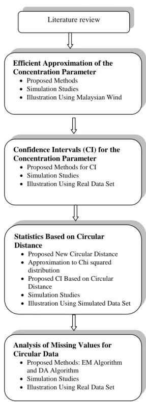
2.6.3 Flow Chart of Research Design of the Study 40
CHAPTER 3: IMPROVED EFFICIENT APPROXIMATION OF
CONCENTRATION PARAMETER FOR VON MISES DISTRIBUTION
3.1 Introduction 43
3.2 Background 43
3.2.1 Parameter Estimation of the Von Mises Distribution 45 3.2.2 Approximation for the Von Mises Concentration Parameter 47
3.3 Proposed Method for Concentration Parameter 48
3.4 Simulation Study 51
3.5 Illustrative Examples 57
3.6 Discussion 59
CHAPTER 4: CONFIDENCE INTERVALS FOR LARGE CONCENTRATION PARAMETER IN VON MISES DISTRIBUTION
4.1 Introduction 60
4.2 Background 60
4.3 Methods in Approximating Confidence Intervals (CI) 62
4.3.1 Percentile bootstrap 63
4.3.2 New Proposed Methods for Confidence Intervals for Concentration
Parameter 65
4.4 Simulation Study 72
4.5 Illustrative Example 79
x CHAPTER 5: A NEW STATISTIC BASED ON CIRCULAR DISTANCE
5.1 Introduction 82
5.2 Approximation to Chi Squared Distribution 82
5.3 Simulation of the Approximated Chi-Squared Distribution 86 5.4 Estimation of Confidence Intervals (CI) for Concentration Parameter, 88
5.4.1 Method 1: Mean 89
5.4.2 Method 2: Median 89
5.4.3 Method 3: Percentile 90
5.5 Simulation Study 91
5.5.1 Confidence Intervals based on percentile 91
5.5.2 Confidence Intervals of Concentration Parameter,
based onMean, Median and Percentile 95
5.6 Illustrative Example 99
5.7 Discussion 100
CHAPTER 6: ANALYSIS OF MISSING VALUES FOR CIRCULAR VARIABLE
6.1 Introduction 101
6.2 Background 101
6.3 Data Imputation of Missing Values for circular data 103
6.3.1 Circular Mean 104
6.3.2 EM algorithm 105
6.3.3 Data Augmentation (DA) algorithm 108
6.4 Simulation Studies 112 6.5 Illustrative Example 131 6.6 Discussion 133 CHAPTER 7: CONCLUSIONS 7.1 Summary 135 7.2 Contributions 137
xi
7.3 Further Research 138
REFERENCES 139
LIST OF PUBLICATIONS 149
LIST OF ORAL PRESENTATIONS 150
Appendix A. Wind direction data recorded at maximum wind speed at Kuala
Terengganu 151
Appendix B. Wind direction data recorded using HF radar and anchored buoy. 152 Appendix C. Programming Script: Simulation study for estimation of
concentration parameter using different methods. 154
Appendix D. Programming Script: Estimation of concentration parameter using
different methods. 155
Appendix E. Programming Script: Confidence Interval for concentration
parameter. 157
Appendix F. Programming Script: CI based on a new statistic 160 Appendix G. Programming Script: Calculating the CI based on a new statistic
(mean, median and percentile) 162
xii
LIST OF FIGURES
Page
Figure 1.1 Arithmetic mean pointing the wrong way 3
Figure 2.1 Flow chart of research design of the study 40
Figure 3.1 Circular plot for residuals 58
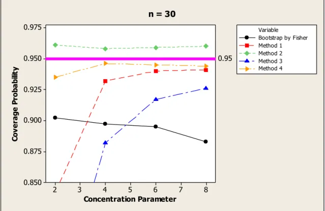
Figure 4.1 Coverage probability versus concentration parameter for n = 30
74
Figure 4.2 Coverage probability versus concentration parameter for n = 50
74
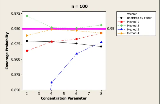
Figure 4.3 Coverage probability versus concentration parameter for n = 100
75
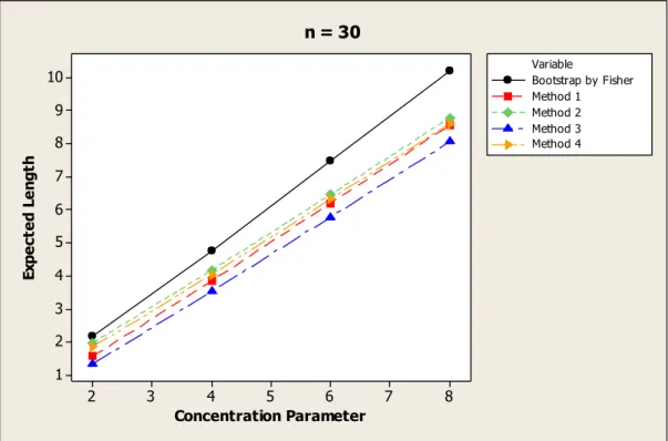
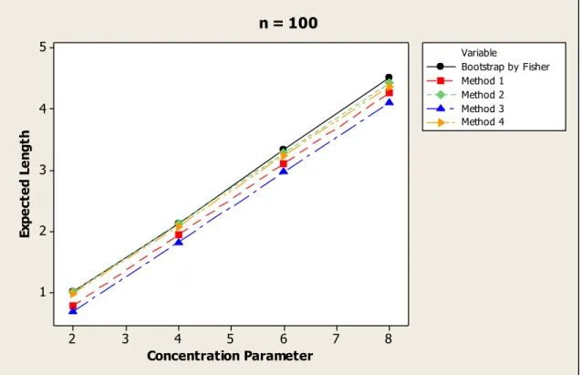
Figure 4.4 Expected length versus concentration parameter for n = 30 77 Figure 4.5 Expected length versus concentration parameter for n = 50 77 Figure 4.6 Expected length versus concentration parameter for
n = 100
xiii
LIST OF TABLES
Page
Table 3.1 Numerical approximation of A
50Table 3.2
Simulation results for various value of parameter
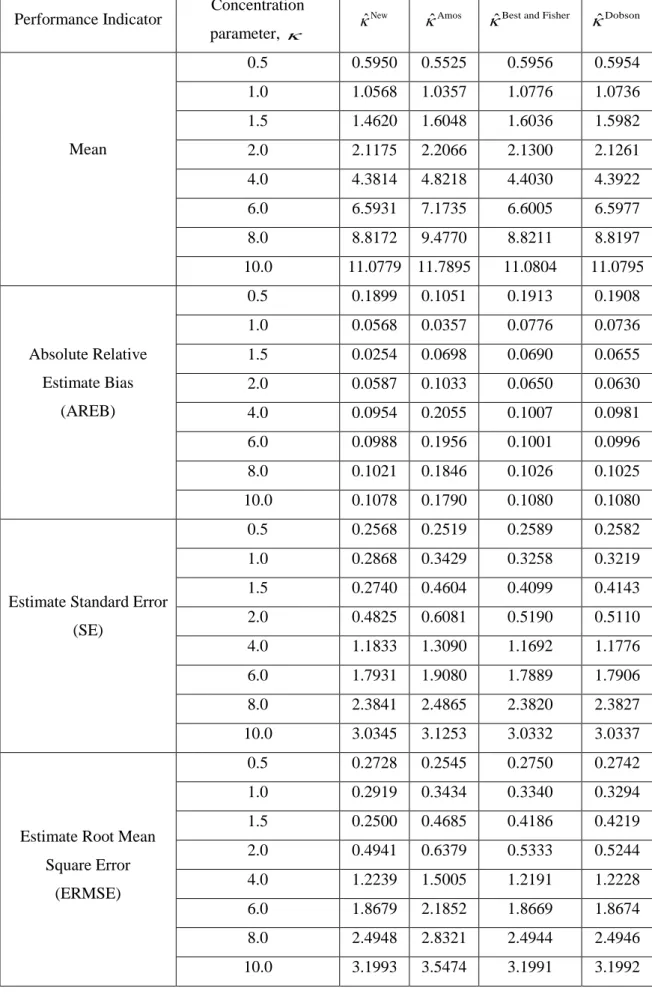
concentration, and n = 30 53
Table 3.3 Simulation results for various value of parameter
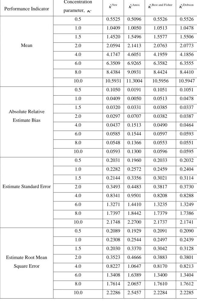
concentration, and n = 50 55
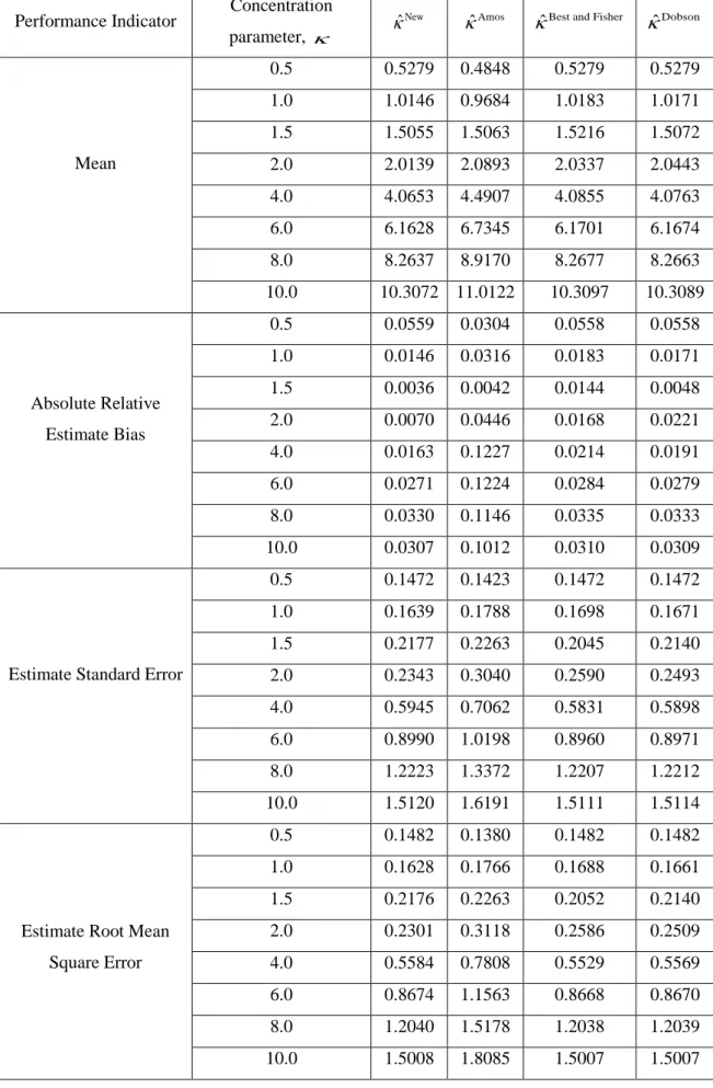
Table 3.4 Simulation results for various value of parameter
concentration, and n = 100 56
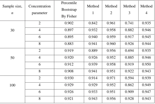
Table 3.5 Estimation of using the new proposed method 58 Table 4.1 Coverage probability for various value of for each
sample size, n = 30, 50 and 100. 73
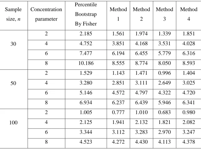
Table 4.2 Expected length for various value of for each sample
size, n = 30, 50 and 100. 76
Table 4.3 Confidence intervals for wind direction data recorded at
maximum wind speed at Kuala Terengganu 80
Table 5.1
The percentage of samples correctly approximated by the Chi-Squared distribution with df
n1
.86
Table 5.2 Coverage probability for each percentage value for CI
based on percentile 92
Table 5.3 Expected length for each percentage value for CI based on
percentile 93
xiv sample size, n = 30, 50, 70 and 100 at 0.05.
Table 5.5
Expected length for various value of for each sample
size, n = 30, 50, 70 and 100 at 0.05. 97
Table 5.6
Confidence intervals for simulated based on new statistic
for circular distance 99
Table 6.1 (a) Simulation results for mean direction for sample size,
n = 30 115
Table 6.1 (b) Simulation results of circular distance for mean direction
for sample size, n = 30 116
Table 6.2 (a) Simulation results of circular mean for mean direction for
sample size, n = 50 117
Table 6.2 (b) Simulation results of circular distance for mean direction
for sample size, n = 50 118
Table 6.3 (a) Simulation results of circular mean for mean direction for
sample size, n = 100 119
Table 6.3 (b) Simulation results of circular distance for mean direction
for sample size, n = 100 120
Table 6.4 (a)
Simulation results of mean for concentration parameter,
for sample size, n = 30 121
Table 6.4 (b) Simulation results of EB for concentration parameter,
for sample size, n = 30. 122
Table 6.4 (c)
Simulation results of ERMSE for concentration
parameter, for sample size, n = 30 123
xv for sample size, n = 50
Table 6.5 (b) Simulation results of EB for concentration parameter,
for sample size, n = 50 125
Table 6.5 (c)
Simulation results of ERMSE for concentration
parameter, for sample size, n = 50 126
Table 6.6 (a)
Simulation results of mean for concentration parameter,
for sample size, n = 100 127
Table 6.6 (b) Simulation results of EB for concentration parameter,
for sample size, n = 100 128
Table 6.6 (c)
Simulation results of ERMSE for concentration
parameter, for sample size, n = 100 129
Table 6.7
Table 6.7: Parameter estimation based on imputation
method 132
Table 6.8 Table 6.8: Circular distance and estimate bias calculated
xvi
LIST OF APPENDICES
Page
Appendix A Wind direction data recorded at maximum wind
speed at Kuala Terengganu 150
Appendix B Wind direction data recorded using HF radar and
anchored buoy 151
Appendix C
Programming Script: Simulation study for estimation of concentration parameter using different methods
153
Appendix D Programming Script: Estimation of concentration
parameter using different methods. 154
Appendix E Programming Script: Confidence Interval for
concentration parameter 156
Appendix F Programming Script: CI based on a new statistic 159
Appendix G Programming Script: Calculating the CI based on
a new statistic (mean, median and percentile) 161
Appendix H
Programming Script: Analysis of missing values
1
CHAPTER 1
INTRODUCTION
1.1 Background
The early studies of circular or directional data date back to the mid of the century in the field of astronomy where it was hypothesised that direction of stars were uniformly distributed (Watson, 1983). Books on methods of analysing circular data in the biological field were published include Batschelet (1981), Zar (1984), Upton and Fingleton (1989) and Cabrera et al. (1991).
In the last 20 years, vigorous development of statistical methods for analysing circular data can be observed in the general statistical methodology with wide application in various fields.
Circular data, however, are somewhat different from linear data due to the different topologies of the circle and the straight line. Angles are recorded in the range (0°, 360°]
degree or [0,2𝜋) radian, then the directions close to the opposite end points are near neighbour in a circular metric but maximally distant in linear metric. The statistical theories for line and circle are very different from one to another because the circle is a closed curve but the line is not. In real life, this kind of data can be easily found in the area of study such as:
i. Meteorology: wind and wave directions (Mardia, 1972; Bowers & Mould, 2000; Caires & Wyatt, 2003; Hussin et al., 2004; Jammalamadaka & Lund,
2 2006; Gatto & Jamalamadaka, 2007; Hassan et al., 2010a and Kamisan et al., 2010)
ii. Medical sciences: the incidence of onsets of a particular disease at various times of the year (Mardia & Jupp 2000).
iii. Biology: bird orientation (Mardia, 1972), animal navigation (Batschelet, 1981) iv. Geology: Azimuths of cross-beds in the upper Kamthi River (Sen Gupta & Rao,
1966)
v. Geography: the direction of the earthquake (Rivest, 1997)
vi. Physics: interference among oscillations with random phases (Beckmann, 1959) vii. Astronomy: orbit plane that can be regarded as a point on the sphere (as
discussed in Watson, 1970)
viii. Criminology: time pattern in crime incidence (Brunsdon & Corcoran, 2005) The circular data cannot be treated as linear data due to its topology. Thus, the needs for statistical analysis as well as making statistical interpretation of this data are really indispensable. For example, as shown in Figure 1.1 for the measurements of wind direction data, the calculated arithmetic mean for 1° and 359° using conventional linear techniques is 180°. On the other hand, by using circular statistics, the mean direction should be 0°. The calculation of the mean direction can be done using the following formula that is totally different from the linear concept.
Circular Mean, 1 1 1 tan 0, 0, ˆ tan 0, tan 2 0, 0, S S C C S C C S S C C
3 Figure 1.1: Arithmetic mean pointing the wrong way
Here, misinterpretation has occurred by someone making their interpretation without having any idea about the circular data. Making this such interpretation will lead to unbiased and misconception in our analysis. As a consequence, a lot of concepts applied in linear statistics are not quite developed for circular statistics.
The von Mises distribution is often used as the basis for parametric statistics inference and will be used in this study. The von Mises distribution, which is also known as the circular normal distribution, is an analogy to the normal distribution in linear data. This study focuses on the estimation of the concentration parameter in von Mises distribution. In this study, we develop an efficient method to approximate the concentration parameter. Later on, we continue with the approximation of the confidence intervals for the concentration parameter. The study of confidence intervals (CI) for parameter in various distributions has gained a lot of attention recently. As for circular data, few studies were done including by Stephen (1969), Fisher (1993), Khanabsakdi (1995 – 1996), Mardia and Jupp (2000) and Jammalamadaka (2001).
In this study, our focus is to find the CI for the concentration parameter in von Mises distribution. A few methods are developed to achieve this objective. The study begins with the approximation method based on circular population, and this is followed by CI based on the asymptotic distribution of ˆ, CI based on the distribution of 𝜃̅ and 𝑅̅
and also CI based on bootstrap-t method. All these methods will be used to construct an
180° 0°
1° 359°
4 efficient CI for the concentration parameter in von Mises distribution. All proposed methods are validated via simulation study and its expected length as well as the coverage probability will be assessed.
Finally, the study also addresses the analysis of missing values for circular data. Missing values is a common problem in data analysis. Deleting or ignoring all missing values, may lead to a lack of statistical power. A few imputation methods have been developed for linear data case, but for circular case, method for handling missing values are still limited. Thus, in this study, two imputation methods are proposed to handle the problem of missing values in circular variables. These two methods are the expectation-maximization (EM) and the data augmentation (DA) algorithm. The analyses are carried out on data that follow von Mises distribution, and the performances of the proposed methods are compared with the conventional method which is the mean imputation method. The biasness are calculated to assess the performance of the proposed method and to identify the most feasible method. Finally, all the proposed methods will be illustrated using real data sets.
5 1.2 Problem Statement
• The von Mises distribution has two parameters namely the concentration parameter and the circular mean. In estimating the parameter, maximum likelihood estimation (MLE) is often used. For the concentration parameter, the solution of the MLE, however, is analytically intractable because of the presence of modified Bessel functions I0
, I1
, ... (Mardia, 1972; Batschelet, 1981 and Fisher, 1993). From the literature, the estimations of concentration parameter are given either for small and large concentration parameter only. Therefore, a new and efficient approximation of concentration parameter which applicable for both small and large concentration parameter is needed.• Most study apply only on simple analysis which is descriptive statistics. The study on inferential statistics, for example, the confidence intervals that can be used in hypothesis testing are relatively few. In circular data, confidence intervals are mostly developed for parameter mean direction only. Therefore, it is necessary to obtain methods for constructing the confidence intervals for concentration parameter.
• Most researchers approach the problem in missing values by deleting or just ignoring them, this may lead to a lack of statistical power. Furthermore, the work on missing values for circular variables are relatively few. Therefore, it is deemed necessary to have methods of addressing the missing value problem for circular data.
6 1.3 Limitation of the Study
In this study, the simulation study was carried out using varies sample size range from 10 up to 500. However, we publish the simulation results up to 100 only. This is because for large sample size, the results always converge beyond the sample size 100. We did not consider the sample size which is more than 500 because of we have limitation in terms of computational time and limited availability of high performance computer to analyse such large data.
1.4 Objective
The main objective of the study is to propose an efficient confidence intervals for the concentration parameter for the von Mises distribution. The followings are the specific objectives of the study:
i. To develop an efficient method of approximating the concentration parameter in von Mises distribution.
ii. To propose new methods of constructing the confidence intervals for the concentration parameter in von Mises distribution.
iii. To propose a new statistic based on circular distance.
iv. To construct the confidence intervals using a new statistic based on circular distance.
v. To formulate a feasible method of imputing missing values for circular variables.
7
CHAPTER 2
LITERATURE REVIEW
2.1 Introduction
This chapter presents the literature review that has led to this study. In Section 2.2, a brief explanation of circular statistics and other studies on circular data are discussed as well as its characteristics. Types of circular distributions are discussed in Section 2.3. The studies on confidence intervals for parameter in circular distribution and related studies are discussed in Section 2.4. In Section 2.5, a review of the methods that are used in handling the missing values for linear data, as well as circular data, are given. The details of the source of data and software used in the study are discussed in Section 2.6 under methodology.
2.2 Circular Statistics
Circular data can be defined as the data distributed on the circumference of the circle. This type of data arises in many fields such as earth sciences, meteorology, biology, physics, psychology, image analysis, medicine and astronomy (Mardia & Jupp, 2000). Many examples of circular data were given in the previous chapter. Further reading on circular data can be found in Mardia (1972), Batschelet (1981), Fisher (1993), Mardia and Jupp (2000) and Jammalamadaka and SenGupta (2001).
8 2.2.1 Numerical Statistics
Let
i where i1, ,n be observations from a random circular sample of sizen. Thus, the descriptive statistics for circular data are described as follows. i. Mean Direction
Each observation of
i is considered as a unit vector and the corresponding values of cos
i and sin
i are calculated. The resultant length which denoted by R is then given by 2 2 R C S , (2.1) where 1 cos n i i C
and 1 sin n i i S
. Thus, the mean direction, denoted by , is given by 1 1 tan if 0 tan if 0 S C C S C C . (2.2)ii. Median Direction
Mardia and Jupp (2000) defined the median as any point where half of the data lie in the arc
,
, and the other half of points are nearer to than . On the other hand, Fisher (1993) defined the median direction as the9 observation that minimise the summation of circular distances to all observations,
1 n i i d
. (2.3)iii. Mean Resultant Length
Mean resultant length denoted by R is defined as the length of the centre of the vector z C iS. R is useful for unimodal data to measure on how concentrated the data is towards the centre. Mean resultant length is given by
R R
n
where 0R1. (2.4)
The data is said to have small dispersion and more concentrated towards the centre if the value of R is close to 1.
iv. Sample Circular Variance
Sample circular variance, denoted by V, is given by
1
V R, where 0 V 1. (2.5) The smaller the circular variance the more concentrated the samples. However, this measure is rarely used in circular statistics in comparison to the measure of the concentration parameter.
10 v. Sample Circular Standard Deviation
Sample circular standard deviation, denoted by v, is given by
2 log 1
v V where V = sample circular variance. (2.6)
vi. Concentration Parameter
Concentration parameter, denoted by , is the standard measure of dispersion for circular data. Best and Fisher (1981) defined the estimate for the concentration parameter obtained by the maximum likelihood method and it is given as follow 5 3 3 2 5 2 , 0.53 6 0.43 0.4 1.39 , 0.53 0.85 1 1 , 0.85 4 3 R R R R R R R R R R R , (2.7)
where R is mean resultant length. The value of lies in the range of
0,
. The large value of indicates that the observations are highly concentrated in the direction of the mean direction . If is close to 0, it shows that the observations are uniformly distributed around the unit circle.Unlike the linear data, circular data cannot be analysed directly using the default and built-in function available in many software. Hence, several researchers have developed statistical packages that can be used in that available software. They have written special programs in few commercial software that later on can easily be used by
11 another researcher. Cox (2001) has developed the programming in Stata that can be used in analysing circular data. Using the package by Cox (2001), the data are assumed recorded in degrees from North. The package consists of four different categories namely utilities, summary statistics and significance tests, univariate graphics and bivariate relationships. Hence, using circular statistics package by Cox (2001) in Stata, the researcher can obtain the descriptive statistics, graphical representation as well as finding the correlation between variables.
Jones (2006) used MATLAB to analysed the directional data. For this purpose, he developed the programs namely Vector_Stats. Specifically, this programs can cater only for two-dimensional directional data such as directions of cross beds. Vector_Stats in MATLAB can be used to calculate the descriptive statistics and generate plots for directional data. The program also provides analysis for single-sample inference on distribution and parameters such as the test of uniformity.
Later on, Berens (2009) developed a MATLAB toolbox for circular statistics namely CircStat. This package includes the descriptive statistics, inferential statistics and measure of association. Apart from that, this toolbox also provides an analysis for data which the underlying distribution is von Mises distribution since this is the most common distribution for circular data. By having this package, the statistical analysis of circular data can be done using MATLAB easily. As for illustration purpose, Berens shows an application on how descriptive statistics can be calculated using neuroscience data.
Lund and Agostinelli were the first who have written programs that is called CircStats package that can be used in analysing directional data in 2007 and later the latest version in 2012 (Lund & Agostinelli, 2012). This package is compatible to use in
12 R and the S-Plus language. It offers a wide range of circular statistical analysis including the descriptive statistics, graphical representations and inferential statistic. The programs written in this package are based on the description in Jammalamadaka and SenGupta (2001).
Apart of developing the package that compatible in analysing the circular data, there are few other software that offer basic statistical analysis for this type of data. Here, we reviewed the studies that have been done using certain softwares to analyse data. Hussin et al. (2006) carried out the circular data analysis using AXIS software (Handeson & Seaby, 2002). AXIS software is an exploratory software that is designed specifically for the directional data. The study focused on how the analysis can be done using the software itself. The analysis included basic summary statistics, circular plot, testing for uniformity or randomness and the comparison between samples. As for illustration purpose, they analysed two different Malaysian wind data set namely Southwest and Northeast.
ORIANA (Kovach Computing Services, 2009) is one of the commercial softwares that offers a basic analysis of circular data. This kind of software is user-friendly as it does not need ones to do the programming in order to carry out the analysis. ORIANA can be used to display the basic summary statistics and it can be very useful for the circular graphical representation as it offers a number of circular plots such as rose diagram, circular histogram, raw data plot and arrow data plot. Testing for uniformity and comparisons between samples also can be done using ORIANA. Hassan et al. (2009) has carried out the analysis of Malaysian wind data using ORIANA and discussed the features that are available to be used for circular statistical analysis.
13 From the studies that were described previously, it showed that this study has gained prior attention from researchers in various fields. This is due to the importance and the wide application of the circular data in many fields such as astronomy, geology, zoology, neuroscience and medical research.
2.2.2 Graphical representation
The graphical representations are often used, to summarise the data and to explore the circular samples. It also useful for the purpose of detecting outliers in circular sample. Below are types of graphical representation that are available for circular samples:
i. Q-Q Plot
Q-Q plot allows us to compare the distribution of two samples. For circular data, the Q-Q plot can be obtained using ORIANA software and using the CircStats package in R or S-Plus.
ii. Spoke Plot
Spoke plot is one of the graphical representation that is specifically useful for circular data. Zubairi et al. (2008) used the MATLAB software to develop this plot. This plot is useful for getting a general pattern of the linear relationship between two circular variables as well as calculating the linear correlation. It consists of inner,
i and outer,
i rings where0
i,
i
360 ,
i
1, 2,
in14 which lines are used to connect the pairs of points
i, i
. As an illustration of this plot, three different Malaysian wind data sets were used, and the correlation, as well as its linear relationship, were calculated in their study.iii. Circular Boxplot
Boxplot is a common plot in real line data set and has been widely used in exploratory data analysis. Boxplot is useful to identify the existence of outliers in the sample. This type of boxplot, however, is not suitable for circular data due to a different topology of the circular data itself. Therefore, Abuzaid et al. (2012) has developed the circular version of boxplot namely as circular boxplot. In order to develop the circular boxplot, median direction, quartile of circular variables and circular interquartile range and fences are calculated.
2.3 Circular Distribution
A circular distribution is a probability distribution that the total probability is concentrated on the circumference of a unit circle. Each point located on the circumference represents a direction. The circular variables,
is measured in radian and in the range of
0, 2
or
,
.15 2.3.1 Uniform Distribution
The uniform distribution which denoted as
U
c is a basic distribution on thecircle. In this distribution, all directions are equally likely. The probability density function (pdf) is given by:
1 2 f , where
0
2
. (2.8)While the distribution function is given by
2
F
, where
0
2
. (2.9)For circular uniform distribution, the mean direction,
is undefined and having mean resultant equal to 0. This distribution plays an important role in circular analysis because they represent the state of ‘no mean direction’ (Jammalamadaka & SenGupta, 2001).2.3.2 Von Mises Distribution
In modelling the circular data, the widely used distribution on the circle is the von Mises distribution. This distribution is also known as the circular normal distribution, and it is an analogue to the normal distribution on the real line. The von Mises distribution is denoted by VM
, where
is the mean direction while is16 the concentration parameter. The probability density function of von Mises distribution (Mardia & Jupp, 2000) is given by
0 1 exp cos 2 f I , 0 2 , 0 , (2.10)where
I
0 denotes the modified Bessel function of the first kind and order 0 and can be defined as:
2
0 0 1 exp cos 2 I d
. (2.11)Von Mises distribution is the most common distribution considered for unimodal samples for circular data. Some of its density properties are:
i. it is symmetrical about the mean direction
ii. it has a mode at
iii. it has anti mode at
.The limiting forms for this distribution as given by Fisher (1993),
i. as 0, the distribution will converge to the uniform distribution, Uc
ii. as , the distribution tends to the point distribution concentrated in the direction of
.17 2.3.3 Wrapped Normal Distribution
The wrapped normal distribution can be obtained by wrapping a normal distribution around a unit circle. This distribution is a symmetric unimodal two parameter distribution. The wrapped normal distribution is denoted by WN
,
where
is the mean direction while is the mean resultant length. The probability density function is given by:
2
1 1 1 2 cos 2 p p f
, 0 2 , 0 1. ( (2.12)If f
is obtained by wrapping a normal distribution with variance 2, then 2 1 2 e
, or 2 2 log . (2.13)The limiting forms for this distribution as given by Fisher (1993),
i. as 0, the distribution will converge to the uniform distribution, Uc
ii. as 1, the distribution tends to the point distribution concentrated in the direction of
.2.3.4 Wrapped Cauchy Distribution
The wrapped Cauchy distribution can be obtained by wrapping the Cauchy distribution on a real line with a density
18
2 2 1 f , (2.14)around the circle. This distribution is a symmetric unimodal two parameter distribution. The wrapped Cauchy distribution is denoted by WC
,
where
is the mean direction while
is the mean resultant length. The probability density function is given by
2 2
1 1 2 1 2 cos f , 0 2 , 0 1. (2.15)The limiting forms for this distribution as given by Fisher (1993),
i. as 0, the distribution will converge to the uniform distribution, Uc
ii. as 1, the distribution tends to the point distribution concentrated in the direction of
.2.4 Confidence Intervals
Confidence intervals can be defined as an interval estimate of the point estimate or the parameter itself. As in Efron and Tibshirani (1993), knowing the interval estimate with its point estimate can say what the best guess is for , and how far in error that guess might be. In the perspective of linear statistics, this area has gained prior attention from many researchers. Many new and integrated approaches were developed to obtain an efficient approximation for confidence intervals based on different methods such as
19 confidence interval based on hypothesis testing, confidence interval based on bootstrap method which include percentile bootstrap, bootstrap-t and iterated bootstrap.
Expected length and coverage are usually used to assess the superiority of the proposed methods to approximate the confidence intervals. Expected length is defined as the class size of the estimated intervals. The coverage probability is the proportion of times that the estimated intervals cover the true parameter. Nominal coverage also known as target value is the confidence level that we consider when approximating the confidence intervals. Coverage error that is defined as the absolute difference between the nominal and actual coverage probability, is often used to assess the superiority of confidence intervals. The reliability of confidence interval is determined by its coverage (Letson & McCullogh, 1998). A good confidence interval should have a coverage probability that is close to a target value (nominal coverage) as well as having small coverage error. In the next section, the bootstrap method, a method that is widely used in constructing the confidence interval will be discussed.
2.4.1 Bootstrap Method
Bootstrap method was proposed by Efron (see Efron, 1979, 1987 and Efron & Tibshirani, 1993) and has gained so much attention and acceptance from researchers in various fields of study. The bootstrap method is procedures that create a number of sub-samples from a pre-observed data set by a simple random sampling with replacement. The sub-samples is then to be used in investigating the nature of the population without having any assumption about them. For the past few years, many studies have been developed on the bootstrap technique and confidence intervals in various research areas
20 (see Hall, 1986, 1987, 1988; Hall & Martin, 1988; DiCiccio & Efron, 1996; Letson & McCullogh, 1998; Polansky, 2000). This computer-based method is very useful in estimating the standard error and bias as well as approximating confidence intervals and other statistical measures (see Efron & Tibshirani, 1986).
How many bootstrap replications need to be considered in order to get a good estimation always becomes a question among researchers. Efron (1979) gives n
Bn
as the possible bootstrap replication. To estimate the standard error, 25 to 250 bootstrap replications usually considered. But, for another estimate such as confidence intervals, number of bootstrap replication will be increased. Bootstrap replications are dependent upon the value of X if n100 and the bootstrap replications is taken to be B10000 (Efron, 1979). As for circular distribution, Fisher (1993) takes number of bootstrap replication, B = 200 to approximate the confidence intervals for the mean direction.
In conclusion, Efron and Tibshirani (1993) gives rules of thumb in determining how many replications should be considered when doing the resampling:
i. Small number of bootstrap replication, for example, B = 25, is usually informative. B = 50 is considered as enough to give a good estimator of standard error.
ii. Very seldom B > 200 bootstrap replications needed in estimating a standard error. The number of replications generally in the range of 25 to 2000.
Efron and Tibshirani (1993) and Chernick (1999) give a comprehensive explanation on constructing the confidence interval based on several bootstrap methods. In this subsection, some reviews on confidence intervals based on various types of the
21 bootstrap method that motivate the study on confidence intervals in circular distribution are discussed.
Porter et al. (1997) and Polansky (2000) studied on bootstrap-t (see Efron, 1982) confidence intervals for small sample size. Porter et al. (1997) applied the non-parametric bootstrap t method to construct the confidence intervals for the mean parameter of an unknown distribution. The non parametric bootstrap is a distribution-free method where the original sample of size n is resampled N times with replacement. The study showed that the bootstrap-t is superior to the other method considered which is the Student’s-t. The superiority of the method is assessed by the coverage probability of each method. The Student’s-t gives a coverage probability that is less than the nominal as opposed to bootstrap-t which has a better coverage probability.
Letson and McCullogh (1998) discussed on different types of the bootstrap method in approximating confidence interval. Five different types of bootstrap techniques are considered which include single and double bootstrap. The performance of each method is assessed by its coverage error. Coverage error is defined as the absolute difference between the nominal coverage (target value) and the actual coverage (coverage probability). Shi’s double bootstrap method is said to be superior because it gives good coverage in comparison to single bootstrapping methods.
Besides that, Polansky (2000) carried out the study on stabilizing the end points of bootstrap-t intervals, as well as its coverage error. This study was done for small sample size. The objective of his study is to improve the stability of the bootstrap-t method and preserve the coverage error. This is because the bootstrap-t is known to have a good coverage error. This method is said to be better as opposed to the
22 estimated-variance-stabilizing method by Tibshirani (1988) which only reduces the expected length but increases the coverage error.
In directional data, the bootstrap method in approximating the confidence intervals for parameter in circular distribution was developed by Ducharme (1985), Fisher and Hall (1992) and Fisher (1993). The details on confidence intervals for parameter in circular distribution will be discussed in the next subsection.
2.4.2 Confidence Intervals for Parameter in Circular distribution
In this subsection, the review on confidence intervals for parameter in circular distribution will be discussed. As explained in the previous subsection, the von Mises distribution is the most common distribution occurs in circular data, and it has two parameters namely the mean direction and concentration parameters.
Firstly, a review on confidence intervals for the mean direction will be discussed. Batschelet (1981) in his book has given the calculation of confidence intervals for mean angle with the samples were drawn from a von Mises distribution. For this purpose, calculation of mean vector length r and mean angle of the sample
are required. The angle of deviation
will be determined based on r and the sample size n which can be referred from the chart given by Stephen (1962a & 1962b) and Brown and Mewaldt (1968). From their study, a 100 1
% confidence interval for the mean is
,
.23 A Monte Carlo simulations study was carried out by Ducharme et al. (1985) to compare the performances of the bootstrap method with the other methods. A total of six different methods and non-parametric confidence cones for the mean direction based on the bootstrap method have been considered. As for performance indicator, coverage probabilities were assessed to compare the superiority of the method. Samples were drawn from different distributions, and they are considering bootstrap replication which is B = 200.
Upton (1986) has given the approximation for confidence interval for the mean direction in von Mises distribution. Two proposed methods in approximating
100 1
% of CI were discussed and conclude that the new methods are preferred for smaller value of n and R. The methods of approximation 100 1
% of CI for the mean direction are given as follows:i. Likelihood-based, R0.9
2
2 2 4 ˆ arccos n R nZ n Z R ii. Likelihood-based, R0.9
2 2 2 exp ˆ arccos Z n n R n R 24 where
Z
is the
point of a
12 distribution.Fisher (1993) described the steps for finding the confidence intervals for the mean direction based on the bootstrap method. He suggested three different techniques to determine the final confidence intervals for the mean direction. The basic method (Technique 1) to obtain a 100 1
% confidence interval for the unknown mean direction as given by Fisheri. calculate
b
ˆ
b*
,
b
, b1, ,Bii. sort into increasing order to obtain
1
Biii. let l = integer part of 1 1
2B
2
and m B 1. Thus, the confidence intervals for
will be given as:
l1,
m
.Zar (1999) has given calculations for confidence intervals for the mean direction. He considered two cases as follow
i. for R0.9 and 2 ,1 2 R N ,
2 2
,1 2 ,1 2 2 4 arccos n n N R N N d R .25 ii. for R0.9
2 ,1 2 2 exp arccos n n N N R N d R .where Rn R N. Considering both cases, the 100 1
% confidence interval for the mean direction is given by
d,
d
.On the other hand, Jammalamadaka and SenGupta (2001) discussed on the construction of confidence intervals for the mean direction based on circular ‘standard error’ of the MLE for ˆ in von Mises distribution. This method is applicable for large
samples where ˆ 1 ˆ ˆ nR
. Hence, a 100 1
% confidence interval for the meandirection is given by ˆ ˆ 2 2 ˆ arcsin ˆ , ˆ arcsin ˆ
.Otieno and Anderson-Cook (2006b) discussed on three different bootstrap methods (Fisher & Hall, 1989) to estimate the confidence intervals for the preferred direction for a single population. The preferred direction that were used are the mean direction, the median direction and the Hodges-Lehman estimate (Otieno & Anderson-Cook, 2006a). A comparison study was carried out using three different types of the bootstrap technique and the performance of the methods were assessed by their coverage probability and expected length.
26 As for the concentration parameter in von Mises distribution, an early study was carried out by Stephens (1969), where several approximation of confidence for small concentration parameter were proposed. Apart from that, Batschelet (1981) has discussed on the confidence interval for the concentration parameter based on the chart given in Stephen (1962a & 1962b) and Brown and Mewaldt (1968).
Confidence intervals for the concentration parameter based on percentile bootstrap method can be found in Fisher and Hall (1992) and Fisher (1993). Steps on percentile bootstrap will be discussed in Chapter 4, and this method is used in the comparison study with our proposed methods.
Khanabsakdi (1995) proposed confidence intervals for the concentration parameter based on chi-squared variable. A 100 1
% confidence intervals for circular variance is given by2 2 2 2 2 , 1 , 2 2 ns ns
The lower and upper limits of the population circular variance are then to be transformed to lower and upper limits of the concentration parameter. This transformation is obtained using the relation between length of the sample mean vector r, sample circular standard deviation s (Batschelet, 1981) and the concentration parameter, . Comparison with the Stephen’s formula has been carried out, and it showed that the method is more efficient than the previous one. However, this method is said to be applicable only when the data is highly concentrated.
27 2.5 Missing Values
Missing values is one of the problems that always occur in data analysis. This problem must be taken seriously because by ignoring or deleting the missing values that exist in our data will affect the statistical power and may lead to the biasness (Little & Rubin, 2002; Tsikriktsis, 2005). Nowadays, the studies of missing data were extensively done by researchers from various fields such as medical (Enders, 2006), environmental (Norazian et al., 2008) and psychology (Baraldi & Enders, 2010) due to the importance of obtaining the complete data analysis.
There are several classifications of missing values. These classifications influence the optimal strategy for working with missing values. Little and Rubin (2002) gave the classification of missing values as follows.
i. Missing completely at random (MCAR)
MCAR occurs when the probability of missing data on a variable X is unrelated to the other measured variables and the values of X itself. MCAR is said to be not really suitable in practice because of the strict assumption that requires the missingness to be unrelated to the study variables (Raghunathan, 2004)
ii. Missing at random (MAR)
MAR occurs when the missingness is related to the other measured variable in the analysis, but not to the underlying values of incomplete variable. MAR is described as systematic missingness where the tendency for missing data is
28 correlated with other study-related variables in the analysis. This type of missingness is said to be most likely happen in real practice as it requires less stringent assumption about the reason for missing data (Baraldi & Enders, 2010).
iii. Missing not at random (MNAR)
The data is said to be MNAR if the probability of missing data is systematically related to the hypothetical values that are missing. It also can be described as the data that are missing based on the would-be values of the missing observations.
In the next subsection, the reviews on methods of handling the missing data are discussed. Further reading on missing data analysis can be found in Schafer (1997), Allison (2002), Little and Rubin (2002) and Baraldi and Enders (2010).
2.5.1 Traditional Approaches in Handling the Missing Values Problems.
Many extensive studies have been done in handling the data set with missing values problems. Before begin with the analysis, one should understand the nature of the missingness that occurs in the data. This is important in order to choose the best technique that can be applied in analysing such data. In this section, some reviews on traditional approaches in handling missing values problems are discussed.
The most common traditional approaches are deletion and replacement procedures (Peugh & Enders, 2004). The easiest way to handle missing values is by
29 deleting those observations with missing values and consequently lead up to ‘complete’ analysis. This is the default method that is usually used in most statistical and computer analysis package including SPSS, S-Plus, R and SAS. Despite simple and easy, this approach will decrease the sample size of the data and at the same time can reduced the power of statistics (Little & Rubin, 2002).
There are two types of deletion techniques. The first technique is the listwise deletion that also known as the complete-case analysis or case-wise deletion. Many reviews on this technique from the past researchers in various fields including Kim and Curry (1977), Tsikriktsis (2005), Peugh and Enders (2004) and Baraldi and Enders (2010). This type of approach tend to be the choice among the researcher because of the simplicity of the method itself whereby it produce the complete data set and the statistical analysis can be done by using standard analysis techniques (Baraldi & Enders, 2010). As stated in Kim and Curry (1977), this method eliminates from further analysis all cases with any missing data. As a result, it gives a large effect in the data where randomly deleting 10% of the data from each variable in a matrix out of five variables can easily cause an elimination of 59% of cases from analysis. In addition, by using listwise deletion it gives a conservative estimate of the parameters and lead to conservative results. By reducing the sample size, it may decrease the statistical power. Hence, this will lead to lack of statistically significant (Tsikriktsis, 2005; Baraldi & Enders, 2010). By using this method, the data are assumed as MCAR, which missingnes is unrelated to all measured variable.
The second technique in deletion procedure is pairwise deletion that is also known as available-case analysis. Pairwise deletion is an alternative approach over the listwise deletion especially for linear models. According to Allison (2002), pairwise deletion is more efficient than listwise deletion because more data are considered in
30 producing the estimates. Similarly, Baraldi and Enders (2010) stated that this pairwise deletion is an improvement over listwise deletion whereby it minimizes the number of cases discarded during the analysis. Monte Carlo studies have shown that listwise deletion gives less accurate estimates of population parameters such as correlations. Pairwise deletion is consistently more accurate than listwise deletion though the differences can sometimes be small (Hippel, 2004; Acock, 2005; Tsikriktsis, 2005).
Other conventional or traditional methods that were always applied by researchers are simple replacement procedure or also known as single imputation method. There are few types of single imputation method including mean imputation, regression imputation, hot deck imputation and many more. The method of imputation uses the idea of fills in the missing values with some possible value. The most common single imputation method is mean imputation. Usually, this type of imputation is simply can be applied while doing the analysis using most of the available statistical softwares such as SPSS, R and S-Plus.
In mean imputation method (Winkler & McCarthy, 2005; Tsikriktsis, 2005; Saunders et al., 2006, Baraldi & Enders, 2010; Hassan et al., 2010b), all missing values will be replaced with the mean of all available observations. Norazian et al. (2008) applied two different types of mean imputation methods namely mean-before-after method and mean-before method. It was found that mean-before-after gives the best result for predicting missing values. The idea of using the mean substitution may be based on the fact that the mean is a reasonable guess of a value for a randomly selected observation from a normal distribution. However, with missing values that are not strictly random, the mean substitution may be a poor guess. According to Acock (2005), mean substitution is especially problematic when there are many missing values. For example, if 30% of the respondents do not answer the question, it means that there are
31 30% of missing values. If a mean sample is substituted for each of them, then 30% of the sample has zero variance on that data. In this method, any type of missingness (regardless of whether data are MCAR, MAR or MNAR) will lead to biasness of any parameter except the mean (Peugh & Enders, 2004).
The second approach in replacement procedure is known as hot-deck imputation (Tsikriktsis, 2005; Saunders et al., 2005). By using this imputation method, we will replace a missing value with the actual score from a similar case in the data set. In this procedure, a correlation matrix is used to determine the most highly correlated variables. Hot deck imputation works very well in the large samples whereby a similar case is easily to identify. However, in order to apply this method, the programming must be written because it is not one of the built-in function in the most common statistical software.
Another method of replacement procedure is regression imputation. Other studies discussed on regression imputation include Hippel (2004), Tsikriktsis (2005), Winkler and McCarthy (2005), Saunders et al. (2006) and Baraldi and Enders (2010). Regression imputation used the idea of substitutes missing values with predicted scores from a regression equation. In comparison to the previous techniques discussed, regression imputation uses the most sources of information to predict the missing values and provide better estimation for missing values. The steps in this approach involve estimating the relationship between the variables, and then uses the regression coefficients to estimate the missing value. The underlying assumption of regression imputation is the existence of a linear relationship between the predictors and the missing variable. Despite the strategy of using information from the complete variables is good. However, this imputation method also produced biased parameter estimates (Baraldi & Enders, 2010). Apart from that, as in Winkler and McCarthy (2005) and
32 Saunders et al. (2006), the problem might occur during the regression imputation. This is because of the difficulty to work out with the equation and also the correlation between the variables may be weak or different relationship may exist. However, this method is easy to apply to linear data since it is already defaults in certain statistical software packages.
Both imputation techniques that are the mean imputation and regression imputation seems to be much better rather than the deletion process. However, they are still lead to biasness because they fail to account for the variability that is present in the hypothetical data values (Baraldi & Enders, 2010). Hence, the researcher makes an attempt to introduce the modern missing techniques in order to provide better estimates as well as reduced the biasness in estimating the parameter for missing value cases. In the next subsection, the modern missing values techniques will be reviewed.
2.5.2 Modern Techniques in Handling the Missing Values Problem.
Apart of traditional approaches, there are a few modern approaches, and some of them are integrated from the traditional approach. Multiple imputation and maximum likelihood can be considered as the modern techniques in handling the missing values problem. Baraldi and Enders (2010) gives a good introduction to modern approaches that can be used for missing data analysis.
Multiple imputation is done by creating several copies of data set, and each of them consists of different imputed values. Many studies were applied the multiple imputation techniques in handling the missing data previously including Acock (2005),
33 Schafer and Schenker (2000), Kofman and Sharpe (2000), Barzi and Woodward (2003), Junninen et al. (2004), Sartori et al. (2004), Enders (2006), Tsechansky and Provost (2007), Baraldi and Enders (2010), Johnson and Young (2011). Generally, the multiple imputation is done using three steps or phases as follows:
i. Imputation phase
In this stage, specified number of data sets