Dissertations and Theses in Statistics Statistics, Department of
8-2017
A Characterization of a Value Added Model and a
New Multi-Stage Model For Estimating Teacher
Effects Within Small School Systems
Julie M. Garai
University of Nebraska-Lincoln, [email protected]
Follow this and additional works at:http://digitalcommons.unl.edu/statisticsdiss
Part of theStatistical Models Commons
This Article is brought to you for free and open access by the Statistics, Department of at DigitalCommons@University of Nebraska - Lincoln. It has been accepted for inclusion in Dissertations and Theses in Statistics by an authorized administrator of DigitalCommons@University of Nebraska -Lincoln.
Garai, Julie M., "A Characterization of a Value Added Model and a New Multi-Stage Model For Estimating Teacher Effects Within Small School Systems" (2017).Dissertations and Theses in Statistics. 19.
MULTI-STAGE MODEL FOR ESTIMATING TEACHER EFFECTS WITHIN SMALL SCHOOL SYSTEMS
by Julie M. Garai
A DISSERTATION
Presented to the Faculty of
The Graduate College at the University of Nebraska In Partial Fullment of Requirements
For the Degree of Doctor of Philosophy
Major: Statistics
Under the Supervision of Professors Walter W. Stroup and Erin E. Blankenship
Lincoln, Nebraska August, 2017
MULTI-STAGE MODEL FOR ESTIMATING TEACHER EFFECTS WITHIN SMALL SCHOOL SYSTEMS
Julie M. Garai, Ph.D. University of Nebraska, 2017 Adviser: Walter W. Stroup, Erin E. Blankenship
At both the national and state level there is increasing pressure to develop metrics to determine if school systems are meeting educational objectives. All states mandate some form of assessment by standardized tests. One method currently used to model student test scores is Value Added Modeling (VAM) which models student scores as a product of classroom and school environments. One VAM approach is the Tennessee Value Added Assessment System (TVAAS) introduced in Knox County, Tennessee. This approach models student gains from year to year longitudinally allowing student scores in the current year to be correlated with previous years. Teacher eects are included in the layered model which estimates the teacher's added value to a student score through best linear unbiased prediction.
Research using VAM typically occurs in school systems with a large number of students (e.g. New York City, Los Angeles, Chicago, etc.) or in statewide assessments that are combined across school districts (e.g. Tennessee). VAM performance in school systems with small numbers of students is unknown.
One common issue with estimation based on small samples is lack of precision. An area of statistics that has developed methodology for small sample sizes is small area estimation. One approach in this area is indirect estimation which links similar subjects together allowing the small groups to borrow strength from each other.
timation techniques with the traditional TVAAS. The performance of both the multi-stage and TVAAS models are studied through data simulated for small school systems. The precision of predicted teacher value added scores is assessed for both modeling methods.
Acknowledgments
First I would like to thank my advisers Walt and Erin. You have taught me that academia is more than research, that people are important and my feelings matter. You have challenged me to do more and be more. You taught me to learn my own limitations and that sometimes the pressure I put on myself is unreasonable. Thank you for your patience, for the hours of advice, and the pieces of your lives that you have shared with me.
Thank you to my committee members Kathy Hanford and Tiany Heng-Moss. I appreciate all of your feedback and support through this process!
I would also like to thank my parents and siblings for your love and support. You have been so understanding. Mom and Dad thank you for teaching me that I am an intelligent woman and that with a lot of hard work I can achieve more than I thought possible. I wish you were here to see this Dad.
Thank you to my husband Matt for cooking food and reminding me to eat, for washing my clothes so I had something to wear, and for going through my code line by line to nd every mistake. You have been the ultimate supporter and my biggest cheerleader. I would not have made it through this process without you. Also I want to thank my dog Luna for barking in the adjacent room as I wrote this dissertation, forcing me to take some breaks and enjoy life a little.
Finally, I want to thank Team Stroup and Danielle for accepting countless phone calls and encouraging me through this process. Also thank you to my pseudo-therapist Stacey Herceg for always listening.
Table of Contents
List of Figures x
List of Tables xii
1 Introduction 1
2 Literature Review 4
2.1 Value Added Model Overview . . . 4
2.1.1 The Appeal of Value Added Modeling and The Modeling Process 4 2.1.2 The TVAAS Model and Associated Assumptions . . . 6
2.1.3 Continued Research Into Assumptions Regarding Student As-sessment . . . 9
2.1.4 Concerns about VAMs . . . 10
2.1.5 Small School Systems . . . 11
2.2 Small Area Estimation . . . 12
2.2.1 Background . . . 13
2.2.2 Model-based Approach to Small Area Estimation . . . 14
2.3 Merging Value Added Modeling and Small Area Estimation . . . 15
3 Modeling Processes 16 3.1 Tennessee Value Added Assessment System . . . 16
3.1.1 A Demonstrating Example of Value Added . . . 16
3.1.2 The TVAAS and Associated Modeling Assumptions . . . 19
3.2 Small Area Estimation . . . 25
3.2.1 Small Areas: An Application in Nebraska . . . 25
3.2.2 General Form of a Small Area Model . . . 27
3.3 Small Area Multi-Stage Modeling Process . . . 29
3.3.1 Stage One . . . 29
3.3.2 Stage Two . . . 30
3.3.3 Stage Three . . . 30
3.3.4 Stage Four . . . 31
3.4 Measuring Model Performance . . . 32
3.5 Cases for Consideration . . . 33
4 A Demonstration of TVAAS and the Multi-Stage Model 35 4.1 The Data . . . 35
4.1.1 Student Data . . . 36
4.1.2 Teacher Data . . . 38
4.1.3 True Teacher VA Scores . . . 40
4.2 Implementing TVAAS . . . 41
4.3 Implementing the Small Area Multi-Stage Model . . . 42
4.3.1 The First Iteration . . . 43
4.3.1.1 Stage One . . . 43
4.3.1.2 Stage Two . . . 43
4.3.1.3 Stage Three . . . 46
4.3.1.4 Stage Four . . . 46
4.3.3 The Final Iteration . . . 48
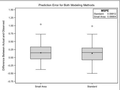
4.4 Comparing Results for the Two Modeling Methods . . . 49
5 A Characterization of the TVAAS and the Multi-Stage Model Via Simulation 52 5.1 Data Generation . . . 52
5.1.1 Generating Teacher Value Added Scores . . . 52
5.1.1.1 Teacher Auxiliary Variables . . . 53
5.1.1.2 Ensuring Simulated Data Are Reasonable . . . 56
5.1.1.3 Design Structure Variables . . . 59
5.1.1.4 Combining Teacher Auxiliary and Design Structure Variables . . . 62
5.1.2 Generating Student Assessment Scores . . . 62
5.1.2.1 Student Raw Scores . . . 63
5.1.2.2 Combining Student Raw Scores with Teacher VAM Scores . . . 64
5.1.2.3 Replicating the Study and Ensuring Simulated Data is Reasonable . . . 65
5.1.3 Dening theZ Matrix . . . 66
5.2 Model Analysis . . . 68
5.2.1 Generated Data . . . 68
5.2.2 Standard Model . . . 69
5.2.3 Small Area Multi-Stage Model . . . 70
5.3 Results . . . 71
5.3.1 Ranking of Teacher Scores . . . 71
5.3.3 Impact of Convergence Criterion . . . 79
5.3.4 Evaluation of Covariance Structure . . . 81
5.4 Conclusions . . . 83
5.4.1 Teacher Rankings . . . 83
5.4.2 Mean Square Prediction Error . . . 84
5.5 Additional Investigations . . . 85
5.5.1 Larger Number of Students Per Grade . . . 85
5.5.2 Future Research . . . 91
6 Conclusions 92 Bibliography 94 Glossary of Terms 99 A Additional Figures of Interest 101 B SAS Code 102 B.1 Setup Macro . . . 102
B.1.1 Simulate Variables and Scores for Case 1 . . . 102
B.1.2 Simulate Variables and Scores for Case 2 . . . 107
B.2 Compile Macro . . . 108
B.2.1 Compile Data Generated Under Case 1 . . . 108
B.2.2 Compile Data Generated Under Case 2 . . . 111
B.3 Analyze Macro . . . 112
B.3.1 Analyze Data Generated Under Case 1 . . . 112
B.3.2 Analyze Data Generated Under Case 2 . . . 124
B.4.1 Simulate Data Under Condition 1 . . . 125 B.4.2 Simulate Data Under Condition 2 . . . 126
List of Figures
2.1 Student Improvement In a Box . . . 5
2.2 Student Growth Above What is Expected . . . 6
3.1 Score for Student i after Grade 1. . . 17
3.2 Score for Student i after Grade 2. . . 17
3.3 Score for Student i after Grade 3. . . 18
3.4 School Systems in Nebraska by Size. . . 27
4.1 Plot of Prediction Error for the Two Modeling Methods . . . 50
4.2 Standard TVAAS Modeling Method Deciles and Heat Map . . . 51
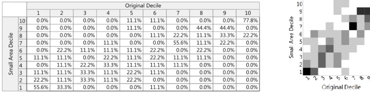
4.3 Small Area Multi-Stage Modeling Method Deciles and Heat Map . . 51
5.1 Years of Service Distribution . . . 57
5.2 Assessing Simulated VAM Scores Under Both Conditions . . . 61
5.3 Assessment Scores for 5 Randomly Selected Students . . . 65
5.4 Student Assessment Scores for 100 Simulated Trials For Each Grade. 66 5.5 Compiled Student Scores Across Grades for Case and Condition. . . 67
5.6 Resulting Deciles for Hypothetical Perfect Model . . . 71
5.7 Resulting Deciles for Standard Method with Case 1 and Condition 1 72
5.8 Results for Both Modeling Methods Under Case 1 and Condition 1 . 74
5.10 Results for Both Modeling Methods Under Case 1 and Condition 2 . 75
5.11 Results for Both Modeling Methods Under Case 2 and Condition 2 . 75
5.12 Comparing MSPE for Modeling Method Based on Cases and Condi-tions used for Generating Data . . . 76 5.13 Condence Interval Plot Comparing Standard and Small Area
Meth-ods . . . 78
5.14 Number of Iterations Required for Dierent Convergence Criterions . 80
5.15 Box plots for the MSPE for Each of the Convergence Criterions . . . 81
5.16 Results for Both Modeling Methods Under Case 1 and Condition 1 for Design 2 . . . 86 5.17 Results for Both Modeling Methods Under Case 2 and Condition 1 for
Design 2 . . . 86 5.18 Results for Both Modeling Methods Under Case 1 and Condition 2 for
Design 2 . . . 87 5.19 Results for Both Modeling Methods Under Case 2 and Condition 2 for
Design 2 . . . 87
5.20 MSPE for Each Case and Condition under Design 2 . . . 89
5.21 30 Students per School, Condence Interval Plot Comparing Methods 90
A.1 Three Negative Binomial Distributions Used to Generate Years of
List of Tables
3.1 Classication System Breakdown in Nebraska[26] . . . 26
4.1 Process Giving Rise to Student Assessment Scores . . . 36
4.2 Portion of Student Data . . . 37
4.3 Process Giving Rise to Teacher VAM Scores . . . 39
4.4 Portion of Teacher Data . . . 40
4.5 True Teacher VAM Scores . . . 40
4.6 Covariance Parameter Estimates after Implementation of TVAAS . . 41
4.7 Fixed Eect Solutions and Teacher Score Estimates . . . 42
4.8 Teacher Data Including Predicted Teacher VAM Scores . . . 44
4.9 Covariance Parameter Estimates and Evaluation of Fixed Eect Sig-nicance . . . 44
4.10 Solution for Fixed Eects After First Iteration . . . 45
4.11 Portion of Solution for Random Eects After First Iteration . . . 45
4.12 Updated Teacher VAM Scores . . . 45
4.13 Predicted Teacher VAM Scores after the Final Stage of the Multi-Stage Model . . . 48
5.1 Converting Years of Service to an Ordinal Variable . . . 54
5.3 Years of Teaching Experience for Public School Teachers, 2011-2012
Academic Year . . . 57
5.4 Years of Teaching Experience for Simulated Teachers . . . 58
5.5 Percentage of Teachers that Fall Into Each Category. . . 58
5.6 Hierarchical Structure under Consideration . . . 59
5.7 Conditions for Variance of Teacher Random Eects . . . 60
5.8 The Z Matrix Incorporated with the Data . . . 68
5.9 Condence Intervals for the True Average Dierence Between Model-ing Methods . . . 79
5.10 Condence Intervals for the True Average Dierence Between Model-ing Methods . . . 79
5.11 Impact of Choice of Convergence Criterion on MSPE . . . 81
5.12 Identifying Appropriate Covariance Structure for Repeated Measure in Standard Model . . . 82
5.13 Condence Intervals for the True Average Dierence Between Model-ing Methods . . . 91
5.14 Condence Intervals for the True Average Dierence Between Model-ing Methods . . . 91
CHAPTER 1 INTRODUCTION
Over the past few decades, there has been a major reform movement to improve eectiveness of primary and secondary education. Specically, there has been a fo-cused eort on accountability assessments at the school and teacher level, particularly with the use of the value added models (VAM). One of these accountability systems was developed in the 1980s in Knox County, Tennessee: the Tennessee Value-Added Assessment System (TVAAS). The TVAAS was mandated as a component of the Education Improvement Act to provide a means of assessing the ability of teachers, schools and systems to meet goals and objectives set forth by the state of Tennessee [32].
Prior to 2001, each state was individually responsible for assessing student knowl-edge and material retention. Several recommendations were put in place at the na-tional level, but not made mandatory in order to allow the states to retain autonomy over their educational processes [15]. With the passage of No Child Left Behind in 2001, local statewide initiatives became subjected to federal mandates. Speci-cally, statewide testing in grades 38 and one grade in high school were required with the goal of holding schools and districts accountable for student progress [6]. The accountability systems introduced were intended to help inform personnel decisions from low stakes evaluations, e.g. needing to participate in professional development
programs, to high stakes evaluations, e.g. bonuses, promotion, and ring of teach-ers [4]. In response, several methods arose as a means of linking student assessment scores to teacher evaluation. A major issue is that the use of the results from the modeling methods introduced, especially for high stakes evaluations, occurred before the models were fully understood. Consequently educational analysts continue to caution consumers (e.g. administrators) about the use of the ndings from student assessment modeling for high stakes decisions. When used properly, the TVAAS and other VAMs have proven to be a valuable tool for modeling student performance.
Many facets of VAMs have been investigated, but most studies focus on urban / suburban school districts where the large number of teachers and students provide more stable value added (VA) score estimates at the teacher, school, and district level [2, 8, 16, 30, 32]. For these current models, the resulting score estimate performance in districts with smaller student / teacher populations is unknown. There is a need to provide smaller school systems with an avenue of measuring student growth and learning.
Traditionally, small area estimation is an area of study within statistics that pro-vides an avenue in cases when small sample sizes lead to ndings with inadequate precision. Indirect estimation is a technique in small area estimation that allows smaller groups of similar subjects to borrow strength from each other by linking the subjects together [29]. In this dissertation we propose a small area multi-stage model that builds on the ndings of the TVAAS by incorporating additional informa-tion about teachers previously unaccounted for in the model. Our two main research questions are
1. How does the TVAAS model, perform in smaller school systems particularly in regards to precision of VA score estimates?
2. How does merging small area estimation techniques with TVAAS through a multi-stage model impact precision of teacher VA score estimates?
Because of the continued research into model assumptions and validity, this disserta-tion aims to provide a useful tool for teacher evaluadisserta-tion and improvement and is not intended to be used for high stakes evaluation purposes namely compensation, hiring, or ring of teachers.
Chapter 2 includes an overview of VAM. We focus on the TVAAS including ongo-ing research and discuss concerns surroundongo-ing VAM. We introduce basic concepts of small area estimation and present a modeling approach that incorporates small area techniques with VAM.
Chapter 3 begins by outlining the form of the TVAAS used for this dissertation including associated modeling assumptions. We proceed by presenting a general form of a small area estimation model that utilizes indirect estimation. Finally we intro-duce the small area multi-stage model that incorporates both TVAAS and small area estimation. We characterize the models under two cases and propose two measures for model comparison.
We include a demonstration of using both the standard TVAAS and small area multi-stage models with simulated data in Chapter 4. We discuss evaluating model convergence and close with a comparison of the ndings between both modeling meth-ods.
Chapter 5 includes an in depth characterization of both the standard TVAAS and small area multi-stage models through simulation. We discuss the process of gener-ating reasonable data, model implementation, results and conclusions. We close this chapter with an additional investigation into the number of students per classroom and our future research plans.
CHAPTER 2
LITERATURE REVIEW
This literature review includes an overview of value added modeling (VAM), with a focus on the Tennessee Value Added Assessment System (TVAAS). We also dis-cuss small area estimation techniques and propose a method for incorporating these techniques with the TVAAS.
2.1 Value Added Model Overview
The principal objective of VAMs is to determine the impact of individual teachers and school systems on student achievement while accounting for characteristics at-tributable to students' backgrounds [1, 8, 23, 32]. With this modeling approach, school systems and teachers are measured on their ability to help students improve rather than their ability to attain a large number of high or procient test scores.
This section discusses the appeal of VAMs along with the process of modeling student improvement. The TVAAS model is introduced along with modeling as-sumptions. We close with current research and concerns about VAM.
2.1.1 The Appeal of Value Added Modeling and The Modeling Process Enthusiasm of using VAMs is that they provide an objective way of estimating teacher impact on student achievement as opposed to solely subjective classroom observation and survey based assessments. Also, teachers are compared relative to each other
rather than a pre-established threshold [13]. VAM is performed through a longitudinal study where multiple years of information are retained for each student. The model links each subsequent grade for a student together, allowing the student to serve as his or her own control and measures the student's progress or improvement rather than the specic score [5, 23, 35]. By measuring progress, rather than prociency, the scores of both low and high achieving students are characterized. Allowing each student to serve as his or her own control accounts for student level inuences, e.g. socioeconomic status or other demographic factors, that inherently aect performance on achievement tests. Consequently the model allows for a clearer picture of the impact of school systems and teachers on student performance.
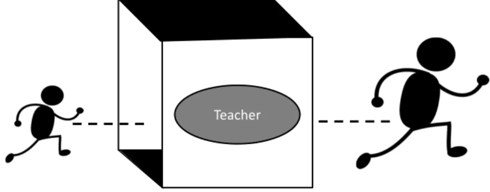
The process of modeling student improvement is well explained by Drayton 2014 and presented in Figure 2.1. A student enters a classroom at the beginning of the
Teacher
Figure 2.1: Student Improvement In a Box
school year represented by a box. The student leaves at the end of the school year with academic growth implying that the box helped the student [10]. The box in this example represents the impact of classroom environment on student learning. This is the basic logic underlying VAM.
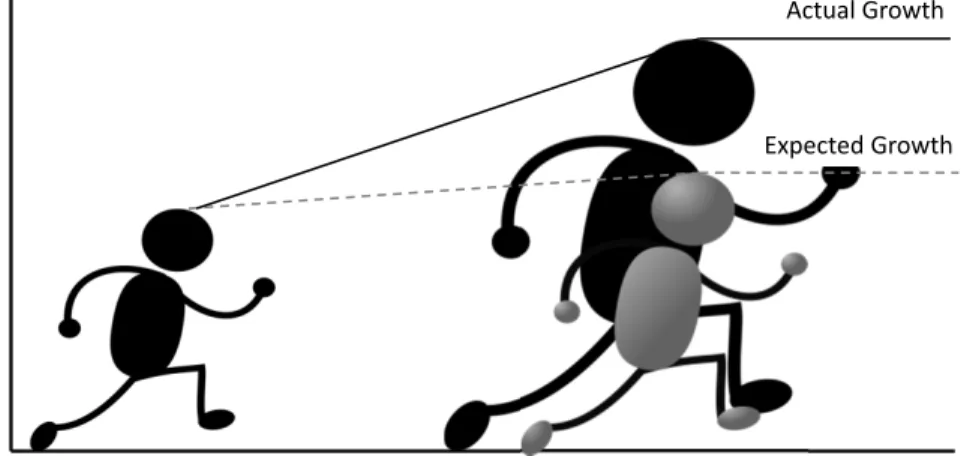
Students are expected to improve each year but any additional growth is attributed to the student's classroom environment, namely the teacher. Figure 2.2 shows the
student growth. If the student grows as expected, we would see the gray gure,
Expected Growth Actual Growth
Figure 2.2: Student Growth Above What is Expected
however the student grows above what is expected and has a higher actual growth represented by the black gure. The additional growth above what is expected is referred to as value added (VA) which is attributed to the teacher [10]. The expected growth is calculated based on the average growth for all students at this grade level. So approximately half of the students grow at a rate below what is expected and half grow at a rate above what is expected. Growth can be positive or negative.
Several models have been proposed for measuring student progress [8, 23]. One method is the TVAAS which was developed in Tennessee [32]. For this dissertation , we have chosen to focus on the TVAAS model which is introduced in more detail in the next section.
2.1.2 The TVAAS Model and Associated Assumptions
The TVAAS is an accountability system that utilizes a multivariate longitudinal anal-ysis of student data and looks at student academic gain from year to year rather than the raw achievement test score [32]. Students are assessed over several grades and in multiple subjects. Along with assessment results, information regarding school
system, teacher and other demographics are recorded annually. The TVAAS allows for student scores over time and scores across subjects to be correlated.
The TVAAS utilizes a layered model to incorporate multiple years of information about each student. The layering allows the inuence of previous teachers on student achievement to persist for subsequent years. Sanders, Saxton and Horn 1997 found that teachers have a signicant eect on student growth [35]. The TVAAS incorpo-rates a teacher eect for the student assessment score that persists undiminished in the model for subsequent grades.
Using mixed model theory for this approach allows for the inclusion of additional covariates in the model known to be correlated with student performance on stan-dardized tests. One criticism of TVAAS is that typically only teachers and school system are identied in the model and covariates known to be correlated with student achievement are omitted, e.g. socioeconomic status, which could lead to biased nd-ings in regards to teachers [16, 20, 21]. Ballou, Springer and Wright 2004 found that the introduction of controls at the student level has a negligible impact on estimated teacher eects in the TVAAS [5]. By measuring student gains or incorporating a baseline measurement, the inclusion of additional covariates provides little additional information and often introduces serious modeling issues namely confounding and multicollinearity. Including additional covariates may seem necessary but end up being redundant if a baseline is included in the model [5].
The layered model incorporates multiple years of information for each student. Fellers 2014 presents an adaptation of the TVAAS model for one tested subject
yi1j1 = µ1+θj1 +i1j1
yi2j1j2 = µ2+θj1 +θj2 +i2j1j2
yi3j1j2j3 = µ3+θj1 +θj2 +θj3 +i3j1j2j3
where yigj1...jg represents student i's test score in year g which includes the overall
mean for year g, µg, as well as the random teacher eects, θjg, for the current year
and previous years if applicable [11]. The model assumes the following teacher eects: θ ∼ Gaussian(0,Iσ2
θ)
residuals: ∼ Gaussian(0,Σ)
with θ and assumed to be uncorrelated. Teacher eects persist in the layered
model undiminished for subsequent years of assessment [5, 8, 11, 14, 23, 34]. Student residuals have a covariance structureΣwhich allows for a repeated measure structure.
Possible structures for Σ are described below.
In the literature both an unstructured covariance structure [5, 14, 23] and rst order auto-regressive covariance structure[11] are used to model the repeated measure structure. Model 2.1.1 incorporates 3 years worth of information for studenti, but
ad-ditional years of information can certainly be incorporated. Also, this model assumes that student ihas the same teacher for the entirety of grade g. This assumption can
be relaxed by incorporating a coecient that allows for multiple teachers per grade [8, 23, 34]. Teacher eect estimates are found using best linear unbiased prediction (BLUP) or shrinkage estimators [5, 8, 11, 14, 22, 23, 34]. Similarly scores can be obtained at the district or state level, depending on the inclusion of this information in the model. Model 2.1.1 is for one tested subject (e.g. Mathematics) which is a simplication of the full TVAAS which typically models multiple tested subjects for student i simultaneously.
In the next section, we discuss continued research being performed into assump-tions made by VAM.
2.1.3 Continued Research Into Assumptions Regarding Student Assess-ment
In addition to model based assumptions (e.g. normality, independence) appropriate use of VAM relies on several other assumptions which are under continuing research. Pauer and Amrein-Berdsley 2014, Rothstein 2009 and Fellers 2014 all explore the assumption that students are randomly assigned to teachers. Pauer and Amrein-Berdsley 2014 investigated the process that administrators follow to assign students to classrooms in Arizona elementary schools. They found that overwhelmingly students are not assigned at random to classrooms. Rothstein 2009 found that bias is present when estimating teacher eects in cases where student assignment to teacher is not random. He determined that the amount of bias present is highly dependent on the quantity of information used to assign students to classrooms. Fellers 2014 found that estimates were not biased under a non-random assignment scheme but did nd that the standard errors were underestimated which could lead to issues with estimate precision.
Another assumption is that the assessment is capable of capturing student growth, specically that students are not subjected to ceiling eects which occur when a number of students score at or near the maximum possible value (it is impossible to score over 100%) which results in minimal cumulative gain. This topic is explored by Koedel and Betts 2010 and Fellers 2014. Koedel and Betts found that typically teacher eect estimates are not severely impacted by the presence of ceiling eects. They did nd an issue with estimation on minimum-competency testing. In these cases, states are solely interested in determining if students have attained a minimum amount of required knowledge from state-wide education objectives. The impact on the results of VAM was more severe for these environments, because a large percentage
of students (e.g. 90%) attained the maximum score. Fellers 2014 determined that The magnitude of bias and eect of ceiling level is not consistent across teachers [11]. Issues arose in cases where a small number of students were at the ceiling and when a large number of students were at the ceiling. In both instances some teacher estimates were unbiased, but at least one teacher estimate showed severe bias.
Koretz 2008 explores the assumption that student test scores are a valid mea-sure of student achievement. One example that he provides is when a mathematics assessment involves extensive reading or writing. While students may be procient mathematically, the test penalizes immigrant students learning a new language. He presents several other examples of how testing alone may not be an adequate measure of student learning.
Many VAMs assume that any missing student records are missing solely at ran-dom. Karl, Yank and Lohr 2013 investigate the impact that this failed assumption has for estimates of teacher impact on student improvement. They introduce a corre-lated random eects model that allows for exploration into the sensitivity of teacher estimates for dierent cases of missing observations. Both patterns of data missing at random and of data not missing at random are investigated. They found that the assumption that the data is missing at random may be violated but that the impact of the violated assumption was minimal when estimating teacher eects in a VAM.
We discuss concerns and criticisms regarding VAM in the next section. 2.1.4 Concerns about VAMs
The American Statistical Association released a statement explaining that VAMs are increasingly promoted or mandated as a component in high-stakes decisions such as determining compensation, evaluating and ranking teachers, hiring or dismissing teachers, awarding tenure, and closing schools [1]. One of the largest concerns
re-garding VAM is not the modeling process but rather the political and micro-political uses of the results [39]. Several articles discuss the implications of using VAM for high-stakes decisions [1, 3, 4, 13, 16, 24]. It is important to note that teacher eects estimated through VAM are estimates with associated standard errors. Consequently it is not advised to use the ndings for high-stakes decisions.
Additionally, several articles discuss the unintended consequences of high-stakes testing. Baker et al. 2010 explain Surveys have found that teacher attrition and de-moralization have been associated with test-based accountability eorts, particularly in high-need schools [3]. Jiang, Sporte and Luppescu 2015 found that teachers had higher levels of stress and anxiety and believed the ndings from the testing process were not worth the added stress [16]. Moore Johnson 2015 explains that heavy re-liance on VAM may lead eective teachers in high-need subjects and schools to seek safer assignments, where they can avoid the risk of low VAM scores. Meanwhile, some of the most challenging teaching assignments would remain dicult to ll and likely be subject to repeated turnover, bringing steep costs for students [24]. High stakes use of VAM results may have more consequences than originally intended.
Instead, many educational analytic researchers suggest using VAM as a tool to help inform program evaluations, to identify teaching practices that result in higher outcomes and potentially use the knowledge for collective education improvement [24, 32]. It is intended that VAM be one means of characterizing academic progress, not the only means.
2.1.5 Small School Systems
The majority of research on VAM is conducted in large school systems. Chetty, Friendman and Rocko 2014 study VAM in New York City School Systems, and Bacher-Hicks, Kane and Staiger 2014 extend the ndings to the Los Angeles Unied
School District [8, 2]. Jiang et al. 2015 discuss VAM in Chicago [16]. Rivkin, Hanushek and Kain 2005 explore VAM across Texas, and Sanders and Horn 1994 investigate across Tennessee [30, 32]. Each of these analyses involve a large number of students and teachers.
Baker et al. 2010 argue that individual classroom results are based on small num-bers of students leading to much more dramatic year-to-year uctuations. Even the most sophisticated analyses of student test score gains generate estimates of teacher quality that vary considerably from one year to the next [3]. Ballou and Springer 2015 echo this sentiment stating that the measures used in... accountability systems are noisy and that the amount of noise is greater the fewer students a teacher has [4]. Ballou and Springer present a brief investigation into the impact of the number of students on estimated teacher eectiveness. However, both articles lack an in depth analysis into the impact of small numbers of students on identication of teacher contribution to student learning. The performance of value added methodology in school systems with small numbers of students has not been investigated.
Additional knowledge about estimation for small sample sizes is needed. One area of statistics specically focuses on developing methodology for cases with small numbers of subjects. Small area estimation is presented in the next section and ties between this area and education are introduced.
2.2 Small Area Estimation
This section includes background information regarding small area estimation and presents a standard form of a small area model.
2.2.1 Background
Sample surveys have long used small area estimation as a means to determine more precise estimates for small groups of interest. The methodology was developed for cases when using traditional estimation techniques on small samples resulted in es-timates with inadequate precision [29]. Often small samples are referred to as small domains which in the education realm may encompass rural school systems as well as school systems in urban / suburban environments where the student and or teacher populations are relatively small. Additionally small area estimation techniques could be useful in larger school systems to determine more precise estimates for smaller subpopulations (e.g. demographics with small representation) within the school.
Rao 2003 introduces indirect estimation as an alternative to traditional estimation. The three types indirect estimation are: domain indirect, time indirect, and domain and time indirect. Domain indirect estimators link related groups of subjects based on similar characteristics at a given time; time indirect estimators link the present and past characteristics for the specic area; domain and time indirect estimators link related areas based on similar characteristics both in the past and the present [29]. Linking similar groups of subjects together allows for borrowing of strength between subjects.
Utilization of indirect estimators introduces sample design bias. If the indirect estimators link similar subjects, the bias will be small leading to a smaller variance in comparison to traditional estimators thus providing an overall reduction in mean square error (MSE). If the linking of subjects is unreasonable, the bias introduced will be large and the overall MSE will be larger in comparison to traditional estimators. It is important to realize that the bias does not go away as sample size increases. A smaller MSE leads to more precise prediction. For the small area model used in this
dissertation the bias arises because we are using shrinkage estimators which are not unbiased in the classical sense but lead to an overall reduction in prediction error.
There are several approaches to small area estimation. This dissertation focuses on model-based estimation which Ghosh and Rao 1994 explain is a special case of a general mixed linear model involving xed and random eects [12]. This approach oers several advantages including the ability to derive optimal estimators, nding measures of variability that can be linked to the individual domains or groups of in-terest, and the exibility to incorporate spatial or time series structures [29]. Several forms of model-based estimation exist in small area estimation. This dissertation fo-cuses on empirical best linear unbiased prediction (EBLUP) estimators because they utilize linear mixed models (LMMs) and a frequentist perspective, a natural pairing with the TVAAS which is also a LMM considered from the frequentist framework. Additional model based approaches discussed in Rao 2003 include parametric empir-ical Bayes estimators and parametric hierarchempir-ical Bayes estimators.
2.2.2 Model-based Approach to Small Area Estimation
Rao 2003 introduces a generic form of an exponential family model that utilizes xed and random eects to provide an estimate of small area numerical summaries (e.g. means, totals, prociencies, etc.) which is shown in Model 2.2.1.
zij =Xijβ+vi+uij (2.2.1)
where j is the number of observational units in subgroup i, vi represents the error
related to linking subjects and uij represents the individual error related to
obser-vational unit j in subgroup i. It is assumed that the error terms vi and uij are
independent withvi iid ∼Gaussian(0, σ2 ν) and uij ind ∼ Gaussian(0, σ2 u).
This model follows similarly from a designed experiment that incorporates random eects with xed eects. Consider zij to be a teacher VAM score, Xij to include
auxiliary variables associated with a teacher which are xed eects, and vi to be a
linking structure that connects teachers possibly based on a sample of locations which is a random eect. Estimation in this case proceeds as with traditional designed experiments as presented in Stroup 2012.
The nal section of this chapter introduces our proposed method of incorporating small area estimation with traditional VAM.
2.3 Merging Value Added Modeling and Small Area Estimation
We aim to incorporate small area estimation techniques with VAM specically TVAAS to incorporate more information about the teachers into our estimates of teacher value added. A linking mechanism can be utilized to link teachers in similar school systems, e.g. small rural environments.
We propose using predicted teacher eects obtained from the TVAAS model using BLUP as our response variable for a small area model. This results in a multi-stage modeling process. We characterize the performance of both the TVAAS and multi-stage model in regards to precision of prediction for teacher value added scores.
CHAPTER 3
MODELING PROCESSES
The chapter begins with the Tennessee Value Added Assessment System (TVAAS), then introduces basic concepts of small area estimation. The nal portion of this chapter introduces the small area multi-stage modeling process and the cases under consideration for the simulation in Chapter 4.
3.1 Tennessee Value Added Assessment System
This section includes a motivating example that introduces terminology and a vi-sualization of the value added process. We then introduce the TVAAS along with associated modeling assumptions.
3.1.1 A Demonstrating Example of Value Added
Consider an example where students begin at 55% on average for a standardized assessment and are expected to gain 2% after each grade, g.
Studentibegins with a baseline score of 50% which is 5% below average. Suppose
after grade g = 1 we have the situation depicted in Figure 3.1 The dotted line
rep-resents the average overall growth for all students which begins at 55%. After grade
1 students grow to 57%, a 2% gain, on average. The expected score for student i
is shown by the dashed line. If the student scores as expected we anticipate a score after grade 1 of 52%, a 2% gain. However, studenti's actual growth is shown by the
45.00% 50.00% 55.00% 60.00% 65.00% 70.00% 75.00% 80.00% 85.00% 0 1 2 3 St a n d a rd iz ed Sco re Grade
Score for Student iafter Grade 1
Average Growth Expected Growth Actual Growth Value added by teacher ݆ଵ
Figure 3.1: Score for Student i after Grade 1.
45.00% 50.00% 55.00% 60.00% 65.00% 70.00% 75.00% 80.00% 85.00% 0 1 2 3 St a n d a rd iz ed Sco re Grade
Score for Student iafter Grade 2
Average Growth Expected Growth Actual Growth
Value added by teacher ݆ଶ
Figure 3.2: Score for Student i after Grade 2.
solid line. Student i scores a 60% which is a 10% gain, 8% above what is expected.
This additional 8% is considered the value added (VA) by teacher j in grade 1.
Figure 3.2 shows the progress of student iafter grade g = 2. If studenti grows at
the rate expected, we anticipate a standardized score of 62%, following the average gain of 2% annually. The dashed line shows the expected growth of student i to
62%. The solid line shows the actual growth of student ito 75%, a gain of 15%. The
additional 13% of growth is considered the VA by teacher j in grade 2.
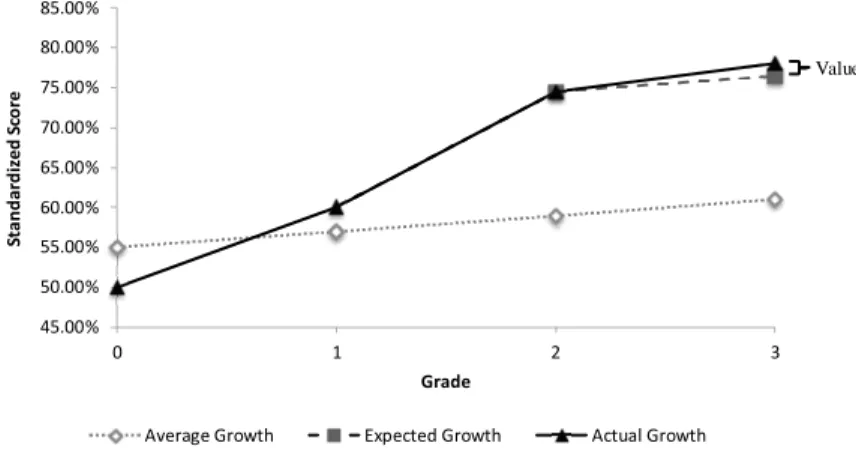
Figure 3.3 shows the results for student i after grade g = 3. If student i grows at
the expected rate, represented by a dashed line, we would expect to see a score after grade3of 77%, a 2% gain. In grade3the actual growth for student i, represented by
45.00% 50.00% 55.00% 60.00% 65.00% 70.00% 75.00% 80.00% 85.00% 0 1 2 3 St a n d a rd iz ed Sco re Grade
Score for Student iafter Grade 3
Average Growth Expected Growth Actual Growth
Value added by teacher ݆ଷ
Figure 3.3: Score for Student i after Grade 3.
the solid line, is 78%, a 3% gain. The additional 1% of growth is the VA by teacher
j in grade 3.
Each of the grades presented in Figures 3.1− 3.3 shows positive VA for each teacher: j1, j2 and j3. It is reasonable for a student to grow at a rate below what
is expected. The expected growth for each student has a central tendency and this growth is compared to the average growth trajectory overall. As a result of assuming normality, 50% of students gain above what is expected and 50% of students gain below what is expected each year. For example if a student improves between grades 1 and 2 at a rate below what is expected (e.g. a 1% gain rather than 2%) this results in negative VA for teacher j for grade g = 2. The TVAAS introduced in Section
dierent teacher, to be the same teacher, or some combination. 3.1.2 The TVAAS and Associated Modeling Assumptions
The Tennessee Value Added Assessment System (TVAAS) utilizes a layered model that incorporates all available years of information for each student. A unique char-acteristic of this model is that teacher eects are considered to be persistent without diminishing over time. Additionally the exibility of the TVAAS allows for all tested subjects for a student to be modeled simultaneously. A baseline measurement for each student is included which allows each student to serve as his or her own control or block factor [32]; because the model is blocked by each individual student, it is redundant to include covariates known to be highly correlated with student success (e.g. socioeconomic factors) in the model [33].
Typically several grades worth of data for each student are stored, including scores on standardized assessments and the teacher the student has for each grade. We denote the rst measured grade of information for student i asg = 1. If the student
is rst assessed in grade 6, in our modelg = 1 will correspond to grade 6. We denote
subsequent years of assessment as g = 1, 2, . . . , Y whereY is the most recent year of
assessment. We use the terms grade and year interchangeably. Model 3.1.1 represents the rst layer for the TVAAS model which corresponds to grade g = 1:
si,1,j1 =µ+Xiβ+tj1 +ei,1,j1. (3.1.1)
For this model, si,1,j1 denotes the standardized test score of studenti in grade g = 1
with teacher j in grade g = 1 for a specic subject (e.g. Mathematics); µ denotes
the common intercept for all students; Xi is the baseline score for student i; β is
represents the individual residual for studentiin gradeg = 1 with teacherj. Sanders
and Horn 1994 discuss the benets of considering teacher eects to be random, such as the exibility to accommodate reality where teachers may teach several dierent grades or switch grades [32]. Thus we assume teacher eects are random with an associated distribution where
tj1 ei,1,j1 ind ∼ Gaussian 0 0 , G 0 R .
The structure of R and Gare discussed below.
Model 3.1.2 shows a general form of the layered model which is an adaptation of models presented in the literature [11, 23, 32]. The total number of measured grades is represented by Y. The general layered model is
si,g,J =µ+Xiβ+ Y X g=1 tjg + Y X g=1 ei,g,J (3.1.2)
where si,g,J denotes the standardized score for student i in grade g with teachers J; µ is the common intercept for all students; Xi is the baseline score for student i
which remains constant for each measured gradeg;β denotes the common regression
coecient;PY
g=1tjg is the sum of the random teacher eects for all previous teachers
and the current teacher, which remain persistent and undiminished in the model for subsequent grades;PY
g=1ei,g,J represents the random residual for studentiafter grade
from 3.1.2 are assumed to have the following distribution t1 t2 ... tw−1 tw ∼Gaussian 0 0 ... 0 0 , G=σj2 1 0 . . . 0 1 0 . . . 0 ... ... 1 0 1 w×w . (3.1.3)
Dening the teacher eects in this manner allows for teachert1to possibly teach grade
g = 1 which we denote t11 or grade g = 2 which we denote t12. Regardless, teacher t1 is the same in both instances. We assume a constant variance across teachers. It
is possible to relax this restriction and allow the teachers to have unique variances. The student residuals from 3.1.2 are assumed to have the following distribution
ei,g,J ∼ 0 0 0 ... 0 , R= σ2 1 σ12 σ13 . . . σ1Y σ2 2 σ23 . . . σ2Y σ2 3 . . . σ3Y ... ... σY2 . (3.1.4)
For grade g = 1 we dene J =j1, for grade g = 2 we dene J =j1j2, and for grade
g =Y we deneJ =j1j2· · ·jY. ThusJ is a compilation of teachers past and present.
Consider an example with a total number of measured grades Y = 3. Model 3.1.2
si,1,j1 = µ+Xiβ+tj1 +ei,1,j1
si,2,j1,j2 = µ+Xiβ+tj1 +tj2 +ei,2,j1,j2
si,3,j1,j2,j3 = µ+Xiβ+tj1 +tj2 +tj3 +ei,3,j1,j2,j3
. (3.1.5)
Here the subscripts 1, 2 and 3 represent the 3 measured grades for studenti. Teacher
eects, tjg, remain in the model for subsequent grades. In year 2, the teacher eect
tj1 from grade g = 1 remains in the model and persists without diminishing. Here
the random teacher eects follow the same distribution presented in 3.1.3. The dis-tribution for the student random residual ei,g,J presented in 3.1.4 simplies to the
distribution presented in 3.1.6 ei,1,j1 ei,2,j1,j2 ei,3,j1,j2,j3 ∼Gaussian 0 0 0 , σ2 1 σ12 σ13 σ2 2 σ23 σ2 3 . (3.1.6)
Assuming an unstructured covariance matrix for student residuals allows for the stu-dent score to vary from year to year and the correlation between scores to vary. An unstructured covariance matrix makes the fewest assumptions about the relationship between current and previous scores [23, 34].
The layered models presented in 3.1.2 and 3.1.5 are a simplication of the full TVAAS model introduced by Sanders, Saxton and Horn 1997. Our models focus on only one subject for each student while the full model incorporates information for all tested subjects and allows for correlation between subjects for each student. Our models also represent a situation where studentihas only 1 teacher for the duration of
classroom teaching or students that have dierent teachers throughout a school year due to transferred classrooms [23].
The matrix form of Model 3.1.2 is s=Xξ+Zt+e
where s = s1,1,J s1,2,J ... s1,Y,J ... sn,1,J sn,2,J ... sn,Y,J (n?Y)×1 for student i= 1, . . . , n in grade g = 1,2, . . . , Y with J =j1 when g = 1 J =j1j2 when g = 2 ... ... J =j1j2· · · jY when g =Y where X= 1 X1 1 X1 ... ... 1 X1 ... ... 1 Xn 1 Xn ... ... 1 Xn (n?Y)×2 and ξ= µ β 2×1
with Z = 1 0 . . . 0 0 0 0 . . . 0 1 1 0 . . . 0 0 0 0 . . . 0 ... ... ... ... ... ... ... ... ... 1 1 . . . 1 0 0 0 . . . 0 ... 0 0 0 . . . 0 1 0 . . . 0 0 0 0 . . . 0 1 1 0 . . . 0 ... ... ... ... ... ... ... ... ... 0 0 0 . . . 0 1 1 . . . 1 (n∗Y)×(w) , t = t1 t2 ... tw w×1
for teacher t= 1, . . . , w, and e= e1,1,J e1,2,J ... e1,Y,J ... en,1,J en,2,J ... en,Y,J (n?Y)×1 .
We assume that t∼ Gaussian(0, G) and e∼ Gaussian(0,R) where G is dened as in 3.1.3 and Ris dened as in 3.1.4. The resulting mixed model equations are
X0R−1X X‘R−1Z Z0R−1X Z0R−1Z+G−1 ξ t = X0R−1s Z0R−1s . (3.1.7)
teachers to student scores. Solving 3.1.7 we obtain teacher VA estimates through best linear unbiased prediction (BLUP). Because G and R are unknown, we utilize restricted maximum likelihood to obtain their estimates. If we dene K as a linear combination of xed eects of interest andMas a linear combination of random eects of interest, we obtain the predictable function K0ξ+M0t by using the estimated values of ξ, ξ˜, and t, ˜t, obtained by solving the mixed model equations [22]. The resulting predictor for teacher j is referred to as the teacher value added model score
or VAM score for teacher j. Ballou, Sanders and Wright 2004, show this process in
detail [5].
Our two objectives with this dissertation are rst to determine how TVAAS per-forms with small sample sizes (e.g. small number of students per classroom and small number of teachers per school) and second to determine how performance is aected by the incorporation of small area estimation techniques. To assess model performance, we are focusing on how accurate the resulting teacher rankings are and how precisely the VAM scores are estimated. This section provides a sucient start-ing place for the rst objective. The next section introduces small area estimation concepts necessary to assess our second objective.
3.2 Small Area Estimation
This section includes an introduction to small area estimation including an example based on the state of Nebraska as well as an applicable form of a small area model. 3.2.1 Small Areas: An Application in Nebraska
Small area estimation is an area of statistics developed for cases where small sample sizes lead to issues with estimation and prediction. One method of small area esti-mation, called indirect estiesti-mation, involves the linking of subjects in a study based
on similar characteristics [29]. Linking subjects increases the eective sample size and allows for borrowing of strength between subjects. If the linking is reasonable the bias introduced by linking subjects together will be small, resulting estimates will be more precise, and there will be a reduction in mean square error (MSE). While linking increases precision, unreasonable linking increases bias even more, osetting increased precision and therefore increasing MSE.
For an example, consider the state of Nebraska. School districts in Nebraska are divided into four classication sizes 2 through 5. Table 3.1 shows the breakdown for the dierent classications. In Nebraska, there is only one school district in Class 4
Classication Number of Inhabitants in the District Total Number of Districts in this Classication 2 <1,000 18 3 1,00199,999 225 4 100,000199,999 1 5 200,000+ 1
Table 3.1: Classication System Breakdown in Nebraska[26]
(Lincoln Public Schools) and one school district in Class 5 (Omaha Public Schools). The largest number of school districts are Class 3.
In the interest of readability, consider a subset of Nebraska public schools. A visual depiction of a possible linking process for 20 public school districts out of 245 total districts is shown in Figure 3.4. The two locations in Nebraska that fall into the largest category are shown with the darkest circle (Class 4 and 5 districts). We have divided Class 3 school districts into two categories. The middle category (identied with gray circles) represents the 85 school districts in Nebraska with at least 500 total students in grades PK-12. The smallest category (identied with white circles) represents Class 2 and small Class 3 school districts in Nebraska, which have less than
School Size
⋯ ⋯ ⋯ ⋯ ⋯
Figure 3.4: School Systems in Nebraska by Size. This picture is adapted from an image available online [7]. 500 total students. 158 school districts in Nebraska fall into this category.
For Figure 3.4, a small area model utilizing indirect estimation may link teachers in similar size school districts (e.g. the white circles) together. This is considered linking based on location [29]. Eectively, teachers deemed to be in similar areas are grouped together. This is especially helpful in smaller school districts where both the number of teachers and number of students per class are small. Other forms of indirect estimation link teachers based on time, e.g. linking the same teacher to previous years of information, or link based on both time and location, e.g. linking teachers based on similar locations and including previous time points.
3.2.2 General Form of a Small Area Model
Once we have established a grouping mechanism (e.g. location) we are able to incor-porate additional information about the teachers not included in the TVAAS model into the estimation process. Several variables are known about teachers (e.g. years of teaching experience, advanced degree, professional development program partic-ipation, etc.); in small area estimation these variables are referred to as auxiliary
variables. A general form of a small area estimation model is
zkl =Ykγ+vk+ukl (3.2.1)
where zkl is the response variable for teacher l within small area k; Yk contains the
auxiliary variables of interest for small area k; γ are the associated parameters of
interest for the auxiliary variables identied in Yk;vk represents the error among the
small areas anduklrepresents the individual error for teacherl within each small area k. It is assumed that vk ukl ind ∼ Gaussian 0 0 , σ2 V 0 σ2 U .
The exibility of this model allows for linking across teachers (e.g. linking teachers from separate schools together), linking within teacher (e.g. linking current year information for teacher l with previous years of information) or a combination of
the two. For our study, we have chosen to focus on two auxiliary variables, level of experience (1-4) and whether or not the teacher has an advanced degree. However, any auxiliary variable deemed to be reasonable can be included. The auxiliary variables chosen for our study are not meant to be exhaustive.
The small area estimation modeling structure can also be viewed as a pseudo-blocking structure. Grouping teachers based on similar characteristics leads to a cluster of similar teachers where the variance within the cluster is small relative to the variance between clusters. The following section discusses the integration of the two models (3.1.2, 3.2.1) presented above.
3.3 Small Area Multi-Stage Modeling Process
The small area multi-stage modeling process begins with the TVAAS then incor-porates additional information about the teachers by using small area estimation techniques. The iterative process combines variables related to the teachers with stu-dent assessment scores in order to obtain more information. Assuming that teacher VAM scores are meaningful, this process aims to address known issues with student assessment data namely imprecise estimates of teacher VA. We seek to determine how incorporating small area estimation aects the resulting teacher estimates and associated precision.
This section introduces the four stages of the small area multi-stage model. • Stage One- Implement TVAAS to obtain estimates of our parameters and
pre-dicted teacher VAM scores, ˆtj
• Stage Two- Use the predicted teacher VAM scores as the response variable for our small area estimation model and obtain new teacher estimates, ˜tj
• Stage Three- Combine the new teacher estimates, ˜tj, from Stage Two with the
parameter estimates from Stage One to obtain new estimated student scores. • Stage Four- Assess model convergence
3.3.1 Stage One
The initial phase of this process involves extracting the teacher VAM scores from equation 3.1.2 using BLUP consistent with the Mixed Model Equations 3.1.7. The obtained teacher VAM scores are denoted ˆtj and are stored along with parameter
estimates µˆ and βˆ. During the rst iteration of the process, ending with Stage One
3.3.2 Stage Two
The teacher VAM scores,ˆtj, obtained in Stage One now act as the response variable.
The two auxiliary variables we are considering for analysis are whether or not the teacher has an advanced degree and level of experience (e.g. teachers with 0-1 years of experience are grouped together). Other or additional auxiliary variables considered to be reasonable could be included in the small area model.
The small area model presented in 3.2.1 is adapted to incorporate our auxiliary variables of interest. Teacher predictions(˜tjklmn)based on the model are stored. The
model for this stage is
ˆ
tjklmo =κ+αm+τo+ατmo+dk+s(d)kl+ujklmo =⇒˜tj (3.3.1)
whereκrepresents the overall mean,αmrepresents the main eect of advanced degree, τo represents the main eect of level of experience, ατmo represents the interaction
between advanced degree and level of experience,dk ands(d)kl are the random eects
due to linking teachers based on location (i.e. district and school within district), and
ujklmo is the residual for teacher j.
3.3.3 Stage Three
Student scores are updated by incorporating parameter estimates obtained in Stage One and teacher predicted scores obtained in Stage Two with baseline scores for the students. The new teacher predicted values˜tj are substituted into the equation from
Stage One for tj along with the predicted values of µˆ and βˆ. The updated model
assessment score of student i. ˆ si,1,j1 = µˆ+Xiβˆ+ ˜tj1 ˆ si,2,j1,j2 = µˆ+Xiβˆ+ ˜tj1 + ˜tj2 ... ˆ si,Y,j1,j2,···,jY = µˆ+Xiβˆ+ ˜tj1 + ˜tj2 +· · ·+ ˜tjY. (3.3.2)
The result is a predicted value for the assessment score of student i in grade g with
teachers J as dened for Model 3.1.2.
3.3.4 Stage Four
We evaluate model convergence after each iteration. Consider ¨si,g,J to be the student
score for the previous iteration andsˆi,g,J to be the score for the current iteration. To
determine convergence, we have chosen to use the average relative change in student scores. If the change falls above the convergence criterion, namely
change= 1 n × 1 Y × n X i=1 Y X g=1 ¨ si,g,J −sˆi,g,J ¨ si,g,J >C (3.3.3)
where student i= 1, . . . , n and grade g = 1, . . . , Y, the multi-stage model continues
into another iteration. If the convergence criterion falls below C, the process
termi-nates and model performance is measured. A discussion of choosing a convergence criterion follows in Section 5.3.3. While we considered the average relative change in student scores as our measure of model convergence, a dierent metric could be utilized.
3.4 Measuring Model Performance
Often a primary goal with VAM is to rank teachers and take appropriate action. For example high ranking teachers are deemed to have the greatest impact on students and school districts may want to determine what can be learned from their methods. The benet of studying these models through simulation is that the true teacher VA is known. If an objective is to identify teachers in the top 10% and teachers in the bottom 10%, we know if the modeling method is correctly identifying these teachers. As one measure of model performance, we rank the teacher VAM scores for both the standard TVAAS model and small area multi-stage model. We then compare the predicted teacher scores for both methods with the true known rankings.
Additionally we can determine how precisely the standard TVAAS model and the small area multi-stage model estimate the true value of each teacher VA score. Consider the true teacher VA score for teacher j to be Tj and ˜tj to be the predicted
teacher VAM score found from one of the modeling methods. The mean square prediction error (MSPE) is calculated as
M SP E = 1 w × 1 Y × w X j=1 Y X g=1 (Tjg −t˜jg)2. (3.4.1)
The MSPE is our second measure of model performance and is found for both the TVAAS and small area multi-stage models. In order to obtain the estimated teacher VAM scores, ˜tj, for each model we
1. TVAAS: store the teacher estimates after Stage One of the rst iteration of the multi-stage model. These are referred to as the predicted scores from the standard method, because TVAAS is currently an approach used in practice. 2. Multi-stage: store the teacher estimates after Stage Two of the most recent
iteration once the multi-stage model has converged. These are referred to as the predicted scores from the small area method, because the multi-stage model incorporates small area estimation.
Dening the MSPE as in formula 3.4.1 is exible and allows for cases when the same teacher has taught multiple grades.
For each of the two modeling methods, the teacher eect estimates, ˜tj, are ranked
and organized into deciles. The resulting teacher deciles are compared with the origi-nal decile to see if the teachers are properly identied. Then all teacher eect estimates are compared to their true original value and the MSPE resulting from Equation 3.4.1 is recorded.
3.5 Cases for Consideration
Because the linking structure for model 3.2.1 is manipulable through data generation and simulation, the impact of the linking structure is assessed. Specically, two cases are considered for analysis:
• Case 1: Teachers linked by auxiliary variables perform similarly, so linking the teachers together is reasonable.
• Case 2: Teachers linked by auxiliary variables perform dierently, and so linking teachers together is unreasonable.
Data generated for Case 1 follow the form of Equation 3.3.1.
For Case 2, while the values of teacher auxiliary variables are still known, those variables do not correlate with teacher VA. The data generated for this case utilize the following model
Here κ represents the overall mean, dk and s(d)kl are the random eects due to
location, and ujklmo is the residual for teacher j. In context, teachers generated
under Case 2 are grouped by level of experience, but level of experience has no bearing on teacher VA. Considering this case allows us to determine the consequences when the auxiliary variables chosen to model teacher VA are independent of teacher VA. Specically we want to assess how the small area method performs when key assumptions made about the linking structure are violated.
In the next chapter, we provide a demonstration of the modeling processes for both the TVAAS and small area multi-stage models. We provide an in depth investigation into the two modeling process through simulation in Chapter 5.
CHAPTER 4
A DEMONSTRATION OF TVAAS AND THE MULTI-STAGE MODEL
This demonstration begins by outlining the scenario that gives rise to the data and the data structure. Discussion includes implementation of the TVAAS along with imple-mentation of the multi-stage small area models including the rst and nal iterations. Relevant results and ndings are presented for both models. The demonstration ends with a comparison of the two modeling methods. We implement these models in SAS/STAT software Version 9.4 of the SAS system for Windows [36]. However the models could easily be implemented using dierent software.
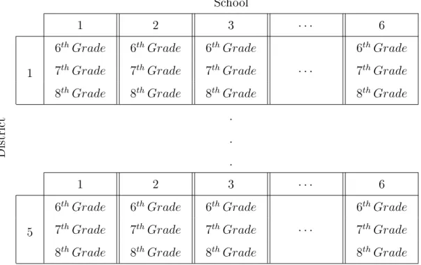
The example that we introduce involves 5 districts each with 6 schools. There are 3 grades at each school each taught by a separate teacher, resulting in 90 total teachers. There are 15 students in each class, thus 450 total students in the sample that are measured for 3 grades, resulting in 1350 scores. The data for this example are simulated by linking teachers based on level of experience and whether or not the teacher has an advanced degree (i.e. under Case 1).
4.1 The Data
There are two sets of data that we are interested in: student data and teacher data. Both are introduced in subsequent subsections.
4.1.1 Student Data
Students are assessed for 3 consecutive years and their scores are recorded. We also have information about where the student began (i.e. a baseline) and the teachers that the student has for each grade. Table 4.1 provides an outline of the process that gives rise to the data following the form of What Would Fisher Do (WWFD) introduced in Stroup 2012 where SV represents the sources of variation [38]. The
What Would Fisher Do Design
Structure SV df TreatmentSV df Combined SV df
teacher 90−1 teacher 89
overall mean 1 overall mean 1
baseline 1 baseline 1
student(teacher) (15−1)∗90 parallels 90∗15−3 student(teacher)
|mean, baseline
1260−2 =1258
Total 1349 Total 1349 Total 1349
Table 4.1: Process Giving Rise to Student Assessment Scores
WWFD process leads to the rst layer of our TVAAS model presented in Model 4.1.1.
si1j1 =µ+Xiβ+tj1 +ei1j1. (4.1.1)
We have 3 years of information for each student, which leads to a model with 3 layers. The full model is presented in 4.1.2
si1j1 = µ+Xiβ+tj1 +ei1j1
si2j1j2 = µ+Xiβ+tj1 +tj2 +ei2j1j2
si3j1j2j3 = µ+Xiβ+tj1 +tj2 +tj3 +ei3j1j2j3
with tj1 tj2 tj3 ind ∼ Gaussian 0 0 0 , σ2 J 0 0 σ2 J 0 σ2J and ei1j1 ei2j1j2 ei3j1j2j3 ∼Gaussian 0 0 0 , σ2 1 σ12 σ13 σ2 2 σ23 σ2 3
Model 4.1.2 is the same as Model 3.1.5 which is introduced in Section 3.1.2.
Table 4.2 shows a portion of the student data for our example. Information regarding the district and school attended by the student is known and included in the data set. Student scores are separated so that one line of the data set represents information about the student for the grade when the score is observed. We have
The SAS System
Obs district school grade teacher student score baseline _Z1 _Z2 _Z31 _Z32 _Z61 _Z62
1 1 1 1 1 1 98.5245 100.117 1 0 0 0 0 0 2 1 1 2 31 1 99.8781 100.117 1 0 1 0 0 0 3 1 1 3 61 1 96.6832 100.117 1 0 1 0 1 0 4 1 2 1 2 1 98.2857 99.453 0 1 0 0 0 0 5 1 2 2 32 1 98.4688 99.453 0 1 0 1 0 0 6 1 2 3 62 1 95.5265 99.453 0 1 0 1 0 1 Page 1 of 1 SAS Output 5/2/2017 file:///C:/Users/jcouton2/AppData/Local/Temp/SAS%20Temporary%20Files/_TD6604_ST...
Table 4.2: Portion of Student Data
information about students from two separate schools. For studentithe baseline score
remains the same for each grade, because it relates to where that student began. The student data set also includes the columns of the Z matrix (reduced to save space). Each column represents a specic teacher. Because the TVAAS is a layered model with persistent teacher eect, all previous year teachers are denoted with a 1 as well as the current year. For example, consider student 1 from school 1. This student