Tax-Benefit Systems in Europe and the US: Between Equity and Efficiency

DISCUSSION PAPER SERIES

Forschungsinstitut zur Zukunft der Arbeit Institute for the Study of Labor

Tax-Benefi t Systems in Europe and the US:

Between Equity and Effi ciency

IZA DP No. 5440

January 2011

Olivier Bargain

Mathias Dolls

Dirk Neumann

Andreas Peichl

Sebastian Siegloch

Tax-Benefit Systems in Europe and the US:

Between Equity and Efficiency

Olivier Bargain

UC Dublin, IZA and CEPS/INSTEAD

Mathias Dolls

IZA and University of Cologne

Dirk Neumann

IZA and University of Cologne

Andreas Peichl

IZA, University of Cologne and ISER

Sebastian Siegloch

IZA and University of Cologne

Discussion Paper No. 5440

January 2011

Any opinions expressed here are those of the author(s) and not those of IZA. Research published in

this series may include views on policy, but the institute itself takes no institutional policy positions. The Institute for the Study of Labor (IZA) in Bonn is a local and virtual international research center and a place of communication between science, politics and business. IZA is an independent nonprofit organization supported by Deutsche Post Foundation. The center is associated with the University of Bonn and offers a stimulating research environment through its international network, workshops and conferences, data service, project support, research visits and doctoral program. IZA engages in (i) original and internationally competitive research in all fields of labor economics, (ii) development of policy concepts, and (iii) dissemination of research results and concepts to the interested public. IZA Discussion Papers often represent preliminary work and are circulated to encourage discussion. Citation of such a paper should account for its provisional character. A revised version may be available directly from the author.

IZA Discussion Paper No. 5440 January 2011

ABSTRACT

Tax-Benefit Systems in Europe and the US:

Between Equity and Efficiency

Whether observed differences in redistributive policies across countries are the result of differences in social preferences or efficiency constraints is an important question that paves the debate about the optimality of welfare regimes. To shed new light on this question, we estimate labor supply elasticities on microdata and adopt an inverted optimal tax approach to characterize the redistributive preferences embodied in the welfare systems of 17 EU countries and the US. Implicit social welfare functions are broadly compatible with the fiction of an optimizing Paretian social planner. Some exceptions due to generous demogrant transfers are consistent with the ignorance of behavioral responses by some European governments and are partly corrected by recent policy developments. Heterogeneity in leisure-consumption preferences somewhat affect the international comparison in degrees of revealed inequality aversion, but differences in social preferences are significant only between broad groups of countries.

JEL Classification: H11, H21, D63, C63

Keywords: social preferences, redistribution, optimal income taxation, labor supply

Corresponding author: Olivier Bargain UCD Belfield, Dublin 4 Ireland E-mail: [email protected] *

We are grateful to A. Spadaro for early collaboration and discussions on this topic, and to discussants & participants to the ZEW Tax Policy workshop (Mannheim), the National Tax Association conference 2010 (Chicago) and several seminars (IZA, FU Berlin, UCD) for useful comments. The usual disclaimer applies. We are indebted to all past and current members of the EUROMOD consortium for the construction and development of EUROMOD and to the NBER for access to TAXSIM. The ECHP and EU-SILC were made available by Eurostat; the Austrian version of the ECHP by Statistik Austria; the PSBH by the University of Liège and the University of Antwerp; the Estonian HBS by Statistics Estonia; the IDS by Statistics Finland; the EBF by INSEE; the GSOEP by DIW Berlin; the Greek HBS by the National Statistical Service of Greece; the Living in Ireland Survey by the ESRI; the SHIW by the Bank of Italy; the SEP by Statistics Netherlands; the Polish HBS by the University of Warsaw; the IDS by Statistics Sweden; and the FES by the UK ONS through the Data

1

Introduction

The level of redistribution via tax and transfer programs di¤ers greatly across countries. Yet does little redistribution in some systems re‡ect more utilitarian views or simply the fact that these countries face tighter e¢ ciency constraints, i.e., redistribution is less easily achieved because of more elastic labor supply? This question paves the debate about the optimality of, and the di¤erences between, welfare regimes in industrialized countries. This paper attempts to address both sides of the same coin by bringing optimal tax theory to the data. We …rst estimate labor supply behavior on harmonized household surveys for 17 EU countries and the US in order to evaluate potential responses. Given these estimated constraints, we then invert the Saez (2002) optimal income tax model to characterize the redistributive preferences embodied in the actual tax-bene…t systems of these countries. This way we can cast usual observations about tax-bene…t systems directly in terms of social welfare language, check whether obtained patterns pass minimum consistency checks (i.e., are compatible with the …ction of an optimizing Paretian planner), and quantify the extent to which inequality aversion truly di¤ers across countries once country-speci…c labor supply behavior is accounted for.

This contribution is the natural follow-up of recent applications of the optimal taxation theory on microdata. The normative literature of the 1970s, following the seminal contribution of Mirrlees (1971), had remained mostly theoretical for lack of reliable information on the ‘true’ distribution of individual abilities. More recently, the increasing availability of representative household datasets has allowed implementing Mirrlees’ models to question the optimality of actual tax-bene…t systems (e.g., in Diamond, 1998, Saez, 2001, 2002). Yet empirical applications remain scarce because little is known about the two fundamental primitives of the model –which are directly related to e¢ ciency and equity concerns –namely labor supply behavior and social preferences, respectively. In most applications some "reasonable" assumptions are usually made for both components.

On the one hand, optimal tax applications most often refer to plausible elasticities as drawn from the labor supply literature. However, even if a relative consensus has been reached on certain aspects – notably that wage elasticities of labor supply are positive, usually smaller than 1 and larger for married women (Blundell and Macurdy, 1999) – there is little agreement on their magnitude. The size of elasticities for a given country can vary greatly depending on the period of investigation or various methodological aspects. Our attempt in this paper is to capture the labor supply responses that are consistent with the same microdata used for optimal tax characterization and estimated in a comparable fashion for all countries.

On the other hand, reasonable levels of social inequality aversion are usually chosen to characterize optimal tax schedules. In the primal problem it is possible to verify which degree of inequality aversion actually makes the optimal schedule closest to the actual one (see Laroque, 2005). Hence, the representation of redistributive preferences for a country at a certain point in time can itself become the object of investigation. In fact, the inverse optimal problem allows directly recovering the redistributive preferences implicit in actual policies. This dual approach

was …rst suggested in the context of optimal commodity taxation (see Decoster and Schokkaert, 1989, among others) and extended to Mirrlees’income tax problem by Bourguignon and Spadaro (2010) in an application on French data. We systematically apply this approach to characterize the equity-e¢ ciency trade-o¤ in many European countries and the US.

A well-known problem with the Mirrlees’model, however, is that it accounts only for behav-ioral responses at the intensive margin.1 The crucial role of the extensive/participation margin has been recognized since Diamond (1980). We adopt here the discrete version of the optimal tax model from Saez (2002), in which the population is partitioned into income groups. This simpli…cation allows both intensive and extensive margins to be incorporated relatively easily. In our empirical analysis, work-consumption preferences are estimated at the individual level and used to calculate elasticities along both margins for the di¤erent income groups.

The present study is also related to two recent contributions. Both of them place emphasis on the question whether transfers should target the workless poor through traditional demogrant policies (means-tested social assistance programs) or the working poor through in-work support. This point is also central to our analysis, as we illustrate how the policy choices made by past governments in Continental/Nordic Europe may reveal little desert-sensitive redistributive pref-erences together with extreme underestimations of participation elasticities.2 _{Firstly, Immervoll}

et al. (2007) suggest an interesting measure of the e¢ ciency cost of marginal transfers from the rich to the poor in 15 EU countries. Under their assumptions of neutral redistributive prefer-ences and uniform elasticities, further redistribution to the workless poor would imply very large e¢ ciency losses in some countries. If governments are ready to bear such costs, this must re‡ect highly Rawlsian social preferences – what we suggest here is a direct characterization of these preferences as revealed by existing tax-bene…t institutions. We also depart from the assumption of uniform elasticities, by retrieving work-consumption preferences consistent with the data, and extend the analysis to the US and several Eastern European countries. Secondly, Blundell et al. (2009) follow the same approach as ours but focus on single mothers in the UK and Germany.3 These two countries are interesting because of contrasted policy choices: in-work support is available for single mothers in the UK, while the German system almost exclusively relies on traditional out-of-work transfers. Our analysis suggests a more systematic characterization and comparison between a large number of countries – yet, like these authors, we also restrict our

1

Most of labor supply adjustments occur, in fact, at the extensive margin, i.e., due to changes in participation decisions (Heckman, 1993). These may be particular strong at the bottom of the income distribution (Eissa and Liebman, 1996; Meyer and Rosenbaum, 2001), which crucially a¤ect the debate about whether redistribution should be directed to the workless poor or to the working poor.

2_{Some authors have already focused on how generous welfare schemes (and con…scatory implicit taxation) at}

the bottom of the distribution could be grounded on the basis of optimal tax formulas in some European countries (see Diamond, 1998, Choné and Laroque, 2005), or in-work support programs (and negative implicit taxation) in the US (Saez, 2002). Our results complete their work by revealing the shape of social preferences that rationalize existing systems under "true" labor supply responses and reasonable variations around them.

3_{Their paper was written at the same time as, and independently from, an ancestor of the present paper,}

analysis to an homogenous population. While policies concerning single mothers may be inspired by non-welfarist objectives (such as minimizing child poverty), we prefer to focus on childless singles in order to extract purely vertical equity concerns as incorporated in tax-bene…t regimes. Our main results are as follows. The inversion procedure shows that tax-bene…t revealed social welfare functions for all countries verify basic properties: in particular they display some taste for redistribution and do not reject the assumption of Paretian governments. Yet the implicit social welfare function is not always concave in Continental/Nordic Europe precisely because of the choice of generous demogrant policies, which imply high e¤ective taxation on the working poor. The assumption that behavioral responses were by and large ignored by govern-ments at the time redistributive schemes were implemented partly corrects these inconsistencies. Interestingly, further corrections can be seen in recent years, mainly due to the introduction of transfers to the working poor. "True" elasticities, i.e., those recovered by econometric estima-tions, may well have come closer to what policy advisors have had in mind in recent years. With these elasticities we …nd that international heterogeneity in work-consumption preferences plays some role – yet our results essentially show that di¤erences in the degree of inequality aversion are signi…cant only across broad groups of countries. Revealed inequality aversion is consistent with direct evidence on citizens’ redistributive views when comparing the US and Continental/Nordic Europe.4

The paper is structured as follows. Section 2 presents the optimal tax model and the inversion procedure. Section 3 describes the empirical labor supply model. Section 4 presents the main elements of the empirical implementation (data, selection, labor supply estimations). Section 5 brie‡y describes the redistributive and incentive potentials of national tax-bene…t systems and discusses the results. Section 6 concludes. In the Appendix we show that results are robust to alternative assumptions regarding the treatment of unemployment bene…ts or the de…nition of income groups.

2

Theoretical Background

2.1 The Optimal Tax Model

The model of Saez (2002) is based on the standard optimal income tax framework. That is, a Paretian government is assumed to maximize a social welfare function subject to an e¢ ciency constraint and a national budget constraint. This function aggregates individual utility levels, which themselves depend on disposable household income (equivalent to consumption in a static framework) and leisure. The form of the social welfare function characterizes the government’s taste for redistribution, ranging from Rawlsian preferences, where the government cares only about the worst o¤ individual, to utilitarian preferences, whereby all individuals are weighted

4

In this line of research our contribution is complementary to studies in which people are asked about their tax preferences and results compared to actual tax schedules (Singhal, 2008, Corneo and Fong, 2008).

equally. Actual productivities are not observed, so that the government can only rely on second-best taxation based on incomes. The e¢ ciency constraint, or incentive-compatibility constraint, states that agents modify their labor supply, and hence their taxable income, in response to the level of e¤ective taxation.

In addition, Saez (2002) assumes that potential workers can be aggregated intoI+ 1discrete groups comprisingI groups of individuals who work, ranked by increasing gross income levelsYi

(i= 1; :::I), and a group i= 0 of non-workers. To each level of market incomeYi corresponds a

level of disposable incomeCi =Yi Ti, whereTi is the e¤ective tax paid by groupi(it ise¤ ective

in the sense that it includes all taxes and social contributions, minus all transfers). Non-workers may receive a negative tax, i.e., a positive transfer T0, identical to C0 by de…nition and often

referred to as a demogrant policy (minimum income, social assistance, etc.). Proportion hi

measures the share of groupiin the population. With this discretized setting, Saez shows that optimal taxation has the following form:

Ti Ti 1 Ci Ci 1 = 1 ihi I X j=i hj 1 gj j Tj T0 Cj C0 fori= 1; :::; I; (1)

with _i and _i the elasticities at extensive and intensive margins respectively, and gi the set

of marginal social welfare weights assigned by the government to groups i = 0; :::; I. Note that Ti Ti 1

Ci Ci 1 is nothing else than

T0

i 1 T0

i in the standard formulation of optimal tax rules, with

T0

i =

Ti Ti 1

Yi Yi 1 the e¤ective "marginal" tax rate (EMTR) faced by group i. It is not exactly

marginal in the usual sense, but is de…ned at the income group level. Formula (1) is very comparable to the usual Mirrlees’rule. In particular, the level of marginal taxation is inversely related to the size of the group and the intensive margin elasticity _i. A noticeable di¤erence, however, is the presence of the extensive margin elasticity _i (see Diamond, 1980). If it is zero, the model is simply a discrete version of Mirrlees and negative marginal tax rates resulting from in-work support –such as the US Earned Income Tax Credit (EITC) –are never optimal, since they discourage productive workers at the intensive margin. However, the larger the extensive elasticity, the more likely are optimal schedules featuring smaller guaranteed income for non-workers and larger in-work support (and possibly negative marginal taxes at low income levels, see Saez, 2002, Choné and Laroque, 2005).

Note also that the de…nitions of the elasticities at the intensive and extensive margins are rather speci…c in the present context. They are de…ned as:

i = Ci Ci 1 hi @hi @(Ci Ci 1) (2) i = Ci C0 hi @hi @(Ci C0) ; (3)

respectively. The former captures the percentage increase in groupiwhenCi Ci 1 is increased

by1%, and is de…ned under the assumption that individuals are restricted to adjust their labor supply to the neighboring choice. The latter, the extensive or participation elasticity, is de…ned

as the percentage of individuals in group i who stop working when the di¤erence between the disposable income out of work and at earnings pointiis reduced by1%.5

Finally in expression (1) social preferences are summarized by the set of weights gi. These

weights mingle the “primitive” social weight, i.e., the derivative of the implicit social welfare function integrated over all the workers within group i, and the individuals’ marginal utility of income (theoretical models often rely on quasi-linear preferences, e.g., in Saez, 2001, so the latter is equal to 1). Hence, as argued by Saez (2002), these weights provide a more direct and transparent interpretation than the primitive weights and are preferably the object of our attention. Indeed, they represent the (per capita) marginal social welfare of transferring one euro to an individual in group i, expressed in terms of public funds. Given this de…nition, Saez’ model does not require the speci…cation of utility functions (since the marginal utility of income is incorporated in gi). The only assumption made on preferences is that there is no income

e¤ect, a traditional restriction in this literature, which is supported by our empirical results as discussed below.6 _{When income e¤ects are ruled out, an additional constraint emerges from}

Saez (2002)’s model that normalizes weights as follows:

X

i

higi= 1: (4)

2.2 Retrieving the Marginal Social Welfare Weights

The inverse optimal tax problem is relatively straightforward. Rather than retrieving the optimal tax schedule under certain assumptions about elasticities and social preferences, as summarized by the set of weights gi, we invert formula (1) to infer weightsgi from the knowledge of income

levels Yi (from the data), tax levels Ti (or disposable incomes Ci = Yi Ti, obtained by

mi-crosimulation) and elasticities (obtained by econometric estimations on the same data). More precisely, expression (1) directly gives the weight on the last group:

gI= 1 I TI T0 CI C0 I TI TI 1 YI YI 1 ; (5) as well as weights gi= 1 i Ti T0 Ci C0 i Ti Ti 1 Yi Yi 1 + 1 hi I X j=i+1 hj 1 gj j Tj T0 Cj C0 (6)

for groups i= 1; :::; I 1, which allows us to derive recursively the weights gI to g1. Finally,

the weight g0 for the group of non-workers is obtained using normalization (4). Weights gi

correspond in part to the marginal social welfare function in the continuous model à la Mirrlees. 5

These elasticities are notably di¤erent from the traditional wage-elasticity of hours (participation) which are de…ned as the increase in working time (participation rate) when wage rates increase by1%.

6

In the empirical part we choose a very ‡exible utility function to estimate labor supply elasticities. Zero income e¤ect is not imposed a priori in our estimation but checked a posteriori. We …nd small or insigni…cant e¤ects, so that the assumption made here is acceptable as a …rst approximation.

Therefore, a necessary condition for the implicit social welfare function to be Paretian, i.e. non-decreasing at all productivity levels, is that weights are positive. We shall check this property in our empirical results.

An important remark must be made at this stage. Both the behavioral elasticities _i and _i and the group sizes hi are endogenous to the tax-bene…t system. This means that proportions

hi observed in the data and elasticities estimated on the same data cannot be used to derive

the optimal tax schedule in Saez’ primal problem, as it is sometimes suggested. Think of a no-tax initial scenario: the social planner sets tax rates optimally according to (1) and given parameters _i, _i,hi in the no-tax situation. Agents would then respond to this policy, so that

elasticities and group sizes (in particular the number of non-workers) would change. This in turn invalidates equation (1), i.e., tax levels are no longer optimal, and the optimal tax rule must be applied again, generating further responses, etc. Clearly, it must be assumed that at least one …xed point exists in which the left and right-hand sides of equation (1) are consistent. When using population shares and elasticities estimated on actual data, the actual tax-bene…t system as deemed optimal is precisely such a …xed point.7 _{In other words, observed shares and}

estimated elasticities can only be used in the dual approach to characterize actual tax-bene…t schedules, but not to derive the optimal tax schedule based on (1) in the primal problem.8

3

Estimations of Labor Supply Behavior

Before recovering social welfare weights on some household microdata, we need to estimate behavioral elasticities _i and _i that are consistent with these datasets. We opt for a discrete choice model of labor supply. It requires the explicit parameterization of consumption-leisure preferences, then utility-maximization is reduced to choosing among a discrete set of possibilities (e.g., inactivity, part-time and full-time). This approach has several advantages in the present context: it allows for ‡exible individual preferences, directly accounts for both participation and working-time decisions, and deals easily with complex tax-bene…t systems that yield non-linear budget constraints and, because of means-tested bene…ts, non-convex budget sets. That is, realistic budget constraints can be incorporated in order to disentangle pure preferences (and …xed costs of work) from policy e¤ects on labor supply choices.

Essentially we follow Hoynes (1996), Aaberge et al. (2002) and van Soest (1995). We specify consumption-leisure preferences using a quadratic utility function, i.e., the utility of household 7_{Saez (2002) makes explicit the condition that endogenous population weights should coincide with empirical}

weights when the optimal schedule coincides with the actual one.

8_{Using the primal problem to derive optimal tax schedules from labor supply estimations would require a}

model where tax formulas are based directly on exogenous preferences (utility functions) rather than endogenous summary elasticity measures as used here (see Blundell and Shephard, 2008). See also exciting developments based on numerical simulations and labor supply estimations to characterize optimal tax schedules (Aarberge and Columbino, 2008) or optimal tax reforms (Creedy and Hérault, 2010).

kchoosing the discrete choice j= 1; :::; J can be written as:

Ukj = Vkj(ckj; hkj) + kj (7)

withVkj(ckj; hkj) = ckckj+ ccc2kj+ hkhkj + hh(hkj)2+ chckjhkj fkj; (8)

with household consumption ckj and worked hourshkj. In the deterministic utility Vkj, coe¢

-cients on consumption and worked hours, namely ck and hk, are household-speci…c as they

vary linearly with several taste-shifters (gender, polynomial form of age, region) and incorpo-rate random components (so the model allows for unobserved heterogeneity and unrestricted substitution patterns between alternatives). The …t is improved by the introduction of …xed costs of work fkj, as in Callan et al. (2009), equal to zero if j = 1 (inactivity) and non-zero

otherwise. These costs also depend on observed characteristics (region and education level, to proxy possible di¤erences in job search costs, see van Soest and Das, 2000) and capture the fact that there are very few observations with a small positive number of working hours.

For each hour choice j, disposable income is calculated as a function ckj = d(wkhkj; mk)

of labor income wkhkj and non-labor income mk. Function d is approximated by numerical

simulation of tax and bene…t rules (tax-bene…t calculators are presented in the next section). Wages wk are calculated using earnings and work hours for workers and Heckman-corrected

predictions for non-workers. Because the model is non-linear, we take the wage rate prediction errors explicitly into account for a consistent estimation.

The deterministic utility is completed by i.i.d. error terms kj for each choice assumed to

represent possible observational errors, optimization errors or transitory situations. Under the assumption that error terms follow an extreme value type I (EV-I) distribution, the (conditional) probability for each household of choosing a given alternative has an explicit logistic form, function of deterministic utilities at all choices. The unconditional probability is obtained by integrating out the disturbance terms (unobserved heterogeneity and the wage error term) in the likelihood. In practice, this is done by averaging the conditional probability over a large number of draws, and the simulated likelihood function can be maximized to obtain all estimated parameters (Train, 2003).

In the present non-linear model, labor supply elasticities cannot be derived analytically. Yet several types of elasticities can be calculated by numerical simulations using the estimated model. First of all, “standard” income and wage elasticities are predicted simply by uniformly increasing non-labor income (which is bottom-coded for all those with zero values) or wage rates by 1 percent and by simulating labor supply responses. We follow a calibration method which is consistent with the probabilistic nature of the model at the individual level. For each household it consists of repeatedly drawing a set ofJ+1random terms from an EV-I distribution, together with unobserved heterogeneity terms of the model in their estimated distribution, which generate a perfect match between predicted and observed choices. The same draws are kept when predicting labor supply responses to an increase in wages or non-labor income. Averaging individual responses over a large number of draws provides robust transition matrices.9 Next,

9

the particular elasticities used in the optimal tax model, as de…ned in expressions (2) and (3), can be obtained in the same fashion but necessitate to re-aggregate behavioral responses at the level of each income group (see also Blundell et al., 2009).

4

Empirical Implementation

4.1 Data, Income and Selection

The fundamental information required by the theoretical model is the e¤ective tax Ti = Yi

Ci, which is the aggregation of all direct taxes and transfers in a given income group. This

information is sometimes available in household microdata but often su¤ers from reporting errors, especially as households do not report correctly the levels of taxes they pay or the transfers they receive. Since it is impossible to obtain administrative data for 18 countries, a reasonable option is to simulate as precisely as possible the levels of disposable incomes by combining bene…t calculators with standard household surveys. For Europe we use EUROMOD, a tax-bene…t calculator designed to simulate the redistributive systems of members of the European Union prior to May 1, 2004 (the EU-15 countries) as well as of several new member states (NMS). This is a unique tool to obtain a complete picture of the redistribution and the incentives to work generated by European welfare regimes. An introduction to EUROMOD, a descriptive analysis of taxes and transfers in the EU countries and robustness checks are provided by Sutherland (2001) and Immervoll (2004). EUROMOD is also used in Immervoll et al. (2007) for EU-15 countries. For the US, tax-bene…t calculations are conducted using TAXSIM, the NBER calculator presented in Feenberg and Coutts (1993) and used in several applications (e.g, Eissa and Hoynes, 2011).10

Data and years of simulations are listed in Table A.1 in the Appendix. For the US we use the CPS– IPUMS for the year 2006, with policy simulation on 2005 incomes. EUROMOD is combined with partly harmonized, microdata on incomes, labor force participation and demo-graphics for each European country. We use datasets for 17 EU countries (Poland, Hungary, Estonia and the EU-15 except Luxembourg) and cover tax-bene…t systems of either years 1998 or 2001 for the EU-15 and of year 2005 for NMS.11 The di¤erent datasets at use respect the basic requirements for our exercise, i.e., they provide a representative sample of the population (and in particular of income distributions), with comparable variable de…nitions across countries and all the necessary information to estimate labor supply behavior. For each household k in

their estimated distributions and, for each draw, by applying the calibration procedure.

1 0

For Europe, country reports are available with detailed information on the input data, tax-bene…t rules and modeling plus validation at the national level at www.iser.essex.ac.uk/research/euromod. For the US, TAXSIM is presented in detail at www.nber.org/~taxsim/.

1 1_{Data are collected over the period 1994-2001 for EU-15, and some adjustments are necessary, as explained}

in Table A.1. Note also that given the enormous task of uprating tax-bene…t calculations for so many countries, we are constrained to use what is available within the EUROMOD project at the time the paper was written. Nonetheless, future developments of the project will certainly allow the extension of our results to more recent data and policy years and more countries.

each country, we are able to calculate the amount of bene…ts the household is entitled to and the taxes and social contributions it should pay, and hence its actual level of disposable income ck

that is reaggregated to form average disposable incomes Ci for groups i= 0; :::; I. We also use

tax-bene…t simulations to calculate the disposable income ckj of household k at each discrete

choice j, in order to proceed with labor supply estimations as explained above.

As in standard labor supply studies, we select potential salary workers in the age range

18 64 (i.e., excluding pensioners, student, farmers and the self-employed). To keep up with the logic of the optimal tax model, we exclude all households where capital income represents more than25%of the total gross income. Most importantly, we focus onsingle men and women without children.12 _{This restricts considerably the scope of the analysis but is in our view a}

necessary and reasonable choice to make, for at least two reasons. Firstly, aggregating di¤erent demographic groups within a social welfare function poses fundamental di¢ culties in terms of interpersonal comparisons (see attempts in Aaberge et al., 2008). Even if (well-behaved) money metric utility measures could be derived to express household welfare in a meaningful common unit – which is far from obvious in the state of the art – the proper equivalence scale to use is unknown. Indeed, this would be the one used by the social planner herself and not any arbitrary equivalence scale that would impose some re-ranking and bias measures of vertical equity (see Lambert and Ramos, 1997).13 _{Focusing on one homogenous demographic group}

at a time – here childless singles – implicitly assumes some separability in the social planner’s program, with a …rst stage redistribution between demographic groups and a second stage with vertical redistribution within homogenous groups. It is also assumed that fertility and partnering decisions are exogenous to tax-bene…t policies. Secondly, it is not at all clear which labor supply elasticities should be used if couples were to be included in the analysis. Immervoll et al. (2007) allocate di¤erent elasticities to di¤erent demographic groups but ignore the issue of joint labor supply decision in couples. As in Blundell et al. (2009), we prefer to focus on one-adult households. Importantly, we show in the empirical results that redistribution analyses conducted on single individuals already re‡ect a good deal of the di¤erences in redistributive potentials across selected countries.

4.2 Income Groups and Income Concepts

We partition the population of each country into a small number of groups,I+ 1 = 6, in order to ease cross-country comparisons. In our baseline, group0is composed of inactive individuals who

1 2

We have considered the alternative choice of focusing on single mothers, as in Blundell et al. (2008). This would o¤er the possibility to include a group which is entitled to EITC-type of transfers in the US, the UK and Ireland. However, sample sizes were too small for several countries to pursue meaningful analysis – especially if we consider that extracting homogenous groups requires focusing on single mothers with the same number of children.

1 3

Muellbauer and van de Ven (2004) retrieve implicit equivalence scales embodied in actual tax-bene…t systems. Along this line, one could consider inverting the optimal tax model on a heterogeneous population in order to retrieve both implicit equivalence scales and social welfare weights. This sounds challenging but is not impossible.

report neither labor income nor replacement income (such as unemployment bene…t). Indeed, contributory bene…ts can be seen as pure insurance in most countries, i.e, where payments are closely linked to workers’past earnings through social security contributions. For that reason, unemployment bene…ts (UB) are interpreted here as delayed salaries and treated stricto sensus

as replacement incomes, i.e., those who receive this insurance are treated as workers in our baseline.14 In our view it would not make much sense to mix in group 0 high-skill workers who receive high levels of UB (when replacement rates are very high, as in Scandinavian countries) together with low-skill workers who live on welfare (social assistance). We make some exceptions to this treatment, however, in the case of the UK, Ireland and Poland. For these countries, UB are paid according to ‡at rates and have no strong link to past contributions, hence are treated as redistribution.15 _{Next, groups i = 1; :::; I are simply calculated as income quintiles among}

workers. In Appendix B we show that results are not too sensitive to alternative choices regarding the treatment of UB recipients and the de…nitions of income groups.

The descriptive statistics of our selected sample are reported in Tables A.2 and A.3 in the Appendix. Since the selected population is relatively homogenous by de…nition, we do not report usual demographic characteristics and essentially focus on the characteristics of the discretized income groups – the main ingredients of the model – including group shares hi, average levels

of gross incomeYi and disposable incomeCi for each groupi= 0; :::I, and e¤ective “marginal”

tax ratesT0

i as de…ned above. The redistributive and incentive characteristics of each national

system as captured in these tables are commented extensively in the section on results.

4.3 Labor Supply Elasticities and Heterogeneity in Individual Preferences

The last component to be used in the inverse optimal tax characterization is the set of behavioral elasticities. In our baseline labor supply model, we make use of a thin discretization withJ = 7

choices, from 0 to 60 hours/week with a step of 10 hours, to capture as much as possible the country-speci…c variations in work hours. Since elasticities are a key component, we have also checked alternative levels of discretization and alternative model speci…cations: results, available from the authors, do not change signi…cantly.16 _{For lack of space, we do not report detailed}

estimates of preference parameters or goodness-of-…t measures for 18 countries –available upon request – but simply comment on our …ndings. Results are relatively standard, in that taste shifters related to age most often display a parabolic pattern and are often, but not systemat-ically, signi…cant. Costs of work are most often signi…cantly positive. Higher education leads

1 4

This is also consistent with the pure supply-side logic of the optimal tax model, in which involuntary un-employment is ignored and job seekers who claim bene…ts are treated as (potential) workers. On the explicit introduction of involuntary unemployment and job search decisions in an optimal tax framework, see Boone and Bovenberg (2004).

1 5

In fact the treatment of unemployment insurance has little e¤ect for these countries since, for singles, payments of UB are very similar to levels of income support. Non-contributory social transfers and contributory UB are described in Tables A.6, A.7 and A.8 in the Appendix and commented in the next section.

1 6

We have also performed estimations on a broader group, including single parents, in order to increase sample size and calculated elasticities for each demographic sub-group.

to lower costs, which can be interpreted as lower job search costs for educated workers (see van Soest and Das, 2000). The pseudo-R2 are at conventional levels and the distribution of actual and predicted frequencies for the di¤erent hour choices compare well.

0

.2

.4

.6

.8

AT1998 BE1998 BE2001 DK1998 FI1998 FI2001 FR

1998 FR 2001 G E 1998 G E 2001 G R 1998 IR 1998 IR 2001 12345 12345 12345 12345 12345 12345 12345 12345 12345 12345 12345 12345 12345 0 .2 .4 .6 .8

IT1998 _{NL2001 PT2001 SP1998 SP2001 UK1998 UK2001}

SW2001 US2005 EE2005 HU2005 PL2005

Mean

12345 12345 12345 12345 12345 12345 12345 12345 12345 12345 12345 12345 12345

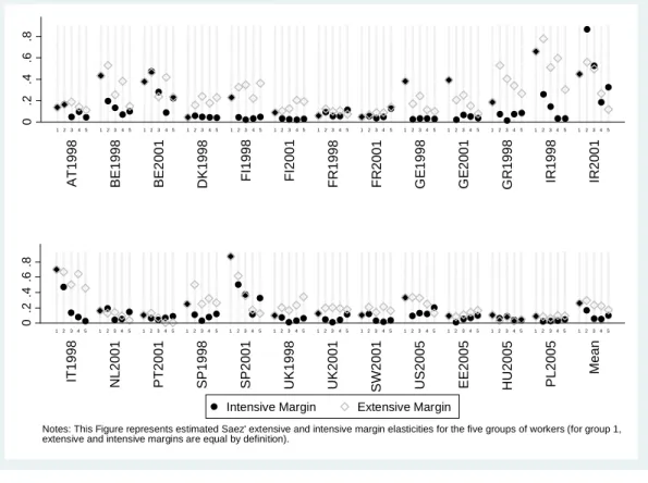
Notes: This Figure represents estimated Saez' extensive and intensive margin elasticities for the five groups of workers (for group 1, extensive and intensive margins are equal by definition).

Intensive Margin Extensive Margin

Figure 1: Saez’Elasticities at the Extensive/Intensive Margins (Point Estimates)

“Standard” income and wage elasticities have been produced in a comparable way for the 18 selected countries. Mean elasticities are reported in the upper panels of Tables A.4 and A.5 in the Appendix. Income elasticities are found to be very small in all countries, often not signi…cantly di¤erent from zero and systematically smaller than :1 in absolute value. A few countries show absolute elasticities between :02 and :06 (Ireland, Hungary, Sweden), others of that same magnitude but statistically insigni…cant (Denmark, Italy), and the elasticities for the remaining countries are smaller than :01. Ignoring income e¤ects in the theoretical model and for the selected population is therefore a reasonable approximation. Wage elasticities of hours and participation are in line with recent evidence based on discrete choice models (see Blundell and Macurdy, 1999, and the meta-analysis of Evers et al., 2008). Yet there is in fact little evidence concerning single individuals because the literature has focused on groups known to be more responsive to …nancial incentives, in particular married women and single mothers. Thus, we provide here some novel evidence concerning labor supply elasticities for single individuals in several industrialized countries. The …rst observation is that our hour

elasticity, which incorporates both change in hours for those in work and the participation e¤ect, is close to the pure participation elasticity. This conveys that also for single individuals, most of the total hour adjustment occurs at the extensive margin. Elasticities are particularly small in France (see Evers et al., 2008), the Netherlands (see Euwals and van Soest, 1999) as well as in Austria (Dearing et al., 2007 report particular low responses, even for married women), Denmark, Portugal, the Netherlands, Hungary and Poland. They are especially large in Spain, Ireland (as supported by Callan et al., 2009) and Italy (particularly large responses in Italy are reported in Aaberge et al., 2002, and Evers et al., 2008). Other countries have intermediary values, which correspond to small elasticities around :1 –:2, for instance in Germany (see also Haan and Steiner, 2000). Estimates are relatively precise and we …nd no systematic di¤erences between (childless) single men and women.

Saez’elasticities at the extensive and intensive margins, i.e., _i and _i, are shown in Figure 1 for the income groups of workersi= 1; :::; I.17 _{Given the speci…c de…nition of these elasticities,}

we do not expect their magnitude to match exactly the standard wage elasticities of hours and participation as discussed above. Yet the marked di¤erences observed across countries mirror previous results with traditional de…nitions, in particular the larger elasticities at theextensive margin in Ireland, Spain and Italy, in contrast to particularly small response in France, Eastern Europe, Portugal and the Netherlands. As expected, most of the extensive margin response is due to groups 1 and 2, the low income groups, then decreases with income levels. As in Blundell et al. (2009), we …nd that elasticities at the intensive margin are much smaller than participation elasticities, except for group 1, for which intensive and extensive elasticities are by de…nition identical (see equations 2 and 3). Together with slightly larger elasticities for the last group, possibly due to backward-bending labor supply, this yields a U-shaped average pattern over the di¤erent quintiles.

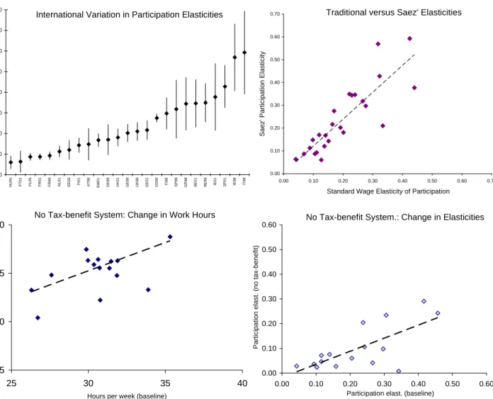
In Figure 2 we provide some useful additional information, focusing on elasticities at the extensive margin. The top-left panel …rst shows con…dence intervals for the mean participation elasticities over income groups i 1, based on bootstrapped standard errors. Estimates appear to be relatively precise in general but 95% con…dence bounds can be as broad as :4 :8 for Italy or :2 :5 for Ireland. As we shall see, this may a¤ect the international comparability of tax-bene…t revealed social inequality aversion. The top-right quadrant compares Saez’partici-pation elasticities with traditionally de…ned elasticities: even if the former are slightly larger, we con…rm there that both types of elasticity capture the international di¤erences in labor income responsiveness. In the lower panels we investigate whether this heterogeneity across countries is genuine or is in fact a¤ected by existing tax-bene…t systems themselves. Indeed, as discussed above, elasticities are endogenous to tax-bene…t policies.18 We suggest a simple experiment to check whether di¤erences in work-consumption preferences actually do matter. Using estimated

1 7

Point estimates and standard errors are reported in the lower panels of Tables A.4 and A.5 in the Appendix.

1 8

In particular, lower participation elasticities for group 1 compared to group 2 in some countries are possibly due to con…scatory EMTRs in that income range that cancel most of the wage/income increment used to calculate elasticities.

The top-left panel represents Saez' participation elasticities averaged over income groups i=1,… ,I (point estimates) and 95% bootstrapped confidence intervals. The top-right panel compares these elasticities with traditionally defined participation elasticities. Lower panels describes a situation with no tax-benefit system (change in hours and participation elasticities).

Traditional versus Saez' Elasticities

0.00 0.10 0.20 0.30 0.40 0.50 0.60 0.70 0.00 0.10 0.20 0.30 0.40 0.50 0.60 0.70

Standard Wage Elasticity of Participation

Saez' Participation Elasticity

International Variation in Participation Elasticities

0.00 0.10 0.20 0.30 0.40 0.50 0.60 0.70 0.80 HU05 PT01 PL05 FR 01 FR 98

NL01 EE05 FI01 AT98 SW

01

DK98 UK01 GE98 UK98 GE01 US06 FI98 SP98 GR98 BE01 BE98 IE01 SP01 IE98 IT98

Saez' P

articipation Elasticity

No Tax-benefit System: Change in Work Hours

25 30 35 40

25 30 35 40

Hours per week (baseline)

Hours per week (no

tax-benefit system)

No Tax-benefit System.: Change in Elasticities

0.00 0.10 0.20 0.30 0.40 0.50 0.60 0.00 0.10 0.20 0.30 0.40 0.50 0.60

Participation elast. (baseline)

Participation elast. (no tax-benefit)

Figure 2: Characterization of Labor Supply Elasticities (Extensive Margin)

preferences we simulate the situation whereby the tax-bene…t system of each country is com-pletely removed (a reform which replaces existing systems with a common ‡at-tax policy yields similar results). As expected, given this radical reform, the bottom-left panel shows an increase in labor supply in almost all countries. This is accompanied, in the bottom-right panel, by a mechanical decrease in elasticities. Most importantly, countries with larger responses in the baseline also tend to have larger responses in the no-tax-bene…t situation. These results thus suggest that individual work-consumption preferences –and possibly also other institutions that may a¤ect …xed costs of work but are not explicitly simulated – are su¢ ciently heterogeneous between countries to explain signi…cant di¤erences in e¢ ciency constraints.

5

Main Results

5.1 National Tax-Bene…t Systems: An Overview

Before presenting the main results, we suggest a brief overview of the redistributive policies in the countries under study. Our comments below are based on Tables A.6, A.7 and A.8 in the Appendix, which give an overview of the rules governing taxes, contributions and transfers for working-age single individuals in the EU and the US. Our aim is to show the diversity of situations that may, to some extent, reveal important di¤erences in political and normative views across countries. For that purpose we present a traditional but suggestive characterization of the redistributive and incentive potential of the di¤erent tax-bene…t systems. For redistributive e¤ects we simply look at inequality as measured by the Gini coe¢ cient.19 E¢ ciency aspects are characterized by implicit taxation on labor income. Both dimensions will be integrated in the optimal tax approach that follows. Detailed results on redistributive policies are provided in Figures A.1 and A.2 in the Appendix, for the whole population and for our selection, respectively. Disincentive e¤ects of taxation are summarized by the EMTRs reported in Appendix Tables A.2 and A.3 and compared graphically in Figure 4 below.

Redistributive E¤ects Graphs in Figures A.1 and A.2 report Gini coe¢ cients of equivalized income and the percentage reduction in Gini due to the tax-bene…t systems. Gini coe¢ cients are shown for four income concepts starting with gross/market incomes and including gradually the di¤erent policy instruments, i.e., bene…ts, social security contributions (SSC) and taxes. Firstly, we can see that the most important redistributive e¤ect for the whole population is on account of transfers.20 Comparing Figures A.1 and A.2 shows that this is also true for our selection of childless singles, but to a lesser extent. In both groups we see that in Nordic countries, the Netherlands, Germany, Belgium and France, bene…ts alone bring the Gini coe¢ cient below the :35mark. In some countries in the middle of the ranking, like Ireland and the UK, bene…ts (and non-contributory income support in particular) also help to reduce considerably the initially high levels of market income inequality. In our selection of working-age singles, redistribution to the poor through means-tested social assistance is substantial in Nordic and Continental Europe but absent in other European countries and the US, with the exception of some disability bene…ts.

SSC levied on earnings, and sometimes on bene…ts, are generally designed as a ‡at-rate scheme, aimed to …nance pensions, health and unemployment insurance, and are relatively neutral in terms of redistribution. The e¤ect of income taxation is more important. Taxes naturally have a larger redistributive impact than transfers in countries where the latter are 1 9_{Gini levels for the whole populations are in line with common wisdom (see Gottschalk and Smeeding, 1997).}

More complete analyses using other inequality/poverty measures or further decomposing the redistributive e¤ect into di¤erent components (e.g., the e¤ect of taxation into tax levels and progressivity e¤ects) can be found in Wagsta¤ et al. (1999).

2 0

This result holds whatever the order in which policy instruments are added to (or withdrawn from) gross income. The order retained here is justi…ed by the fact that bene…ts are taxable in some countries (so that certain combinations, such as gross income minus SSC and taxes, would lead to negative incomes).

small (e.g., Hungary or the US). They sometimes have a signi…cant role even when bene…ts are generous (e.g., in Denmark). Tax structures in almost all of the countries are progressive, with the exception of ‡at tax schemes in Baltic countries (represented here by Estonia). Low earners do not usually pay taxes thanks to tax allowances or tax-free brackets. The degree of vertical redistribution due to income tax schedules depends on a complex mix of tax level, tax progressivity and scope (tax base), as studied in Wagsta¤ et al. (1999). International rankings on the levels of public spending (and in particular spending on redistribution) mirror tax levels, with lower taxation in Southern and Eastern Europe and the US at one end and high tax redistribution in Nordic countries at the other.

Figure 3 provides important additional information. In the left panel we plot the Gini-reduction e¤ect of tax-bene…t policies as previously de…ned, i.e., which include unemployment bene…ts (UB) as part of the redistribution function, against the same e¤ect when UB are treated as market income. We see that the international ranking is broadly preserved: countries with high levels of redistribution through the tax-bene…t system alone are also countries with higher rates of replacement incomes. Nonetheless, the high replacement rates of UB in countries like Denmark make the system even more redistributive than when the sole tax-bene…t policies are accounted for. As argued before, we shall treat UB as pure insurance in our main results in order to be consistent with the logic of the optimal tax model. The right panel of Figure 3 compares Gini reductions in two di¤erent samples: our selection of working-age childless singles versus the whole population. As expected more redistribution occurs in the full population, in particular because of in-work support programs like those operated in the US (EITC) and the UK (WFTC) or demogrant policy targeted at single parents (such as the TANF in the US). Interestingly, however, the …gure shows a high correlation: countries which do not redistribute much among childless single individuals do not redistribute much in general. This is reassuring for what follows: our selection is certainly restrictive but captures well the redistributive intentions of social planners in terms of pure vertical equity.

Incentive E¤ects Turning to the incentive e¤ect of tax-bene…t systems, we directly use EMTRs as previously de…ned at the income group level, i.e., Ti Ti 1

Yi Yi 1, rather than at the

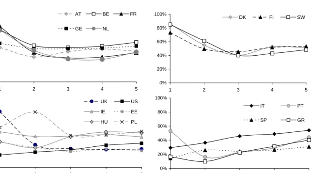
in-dividual level (as, e.g., in Immervoll et al., 2007). The characterization is nonetheless very much in line with previous international comparisons (see Immervoll, 2004). In Figure 4 the upper quadrants show that in Continental (left) and Nordic (right) European countries, EMTRs are larger in upper income groups, due to progressive taxation. In addition, they are particularly large for group 1 (and sometimes group 2). Such high implicit taxation on poor workers is due to high withdrawal rates of means-tested social assistance programs together with the absence of transfers to the working poor (they are excluded from any form of redistribution for the years under consideration, with a few exceptions). Combining the two factors explains a U-shaped pattern of EMTRs extensively discussed in the literature (Bourguignon, 1999, Immervoll, 2004,

BE01 SW97 BE99 DK95 AT98 SW01 FR01 FI98 GE01 GE98 NL00 FI01 UK95 UK01 HU05 IE00 FR98 IT95 IE94 SP96 EE05 PT01 SP00 US06 PL05 GR95 0 .1 .2 .3 .4 .5 % G in i re duct ion du e to tax-be nef it sys tem 0 .1 .2 .3 .4 .5 % Gini reduction due to UB + tax-benefit system

BE01 SW97 BE99 DK95 AT98 SW01 FR01FI98 GE01 GE98 NL00 FI01 UK95 UK01 HU05 IE00 FR98 IT95 IE94 SP96_EE05 PT01 SP00 US06 PL05 GR95 0 .1 .2 .3 .4 .5 .6 % G in i re duct ion ( fu ll sam pl e) 0 .1 .2 .3 .4 .5 .6 % Gini reduction (working age childless singles)

Figure 3: Vertical Redistribution: Impact of Unemployment Bene…ts and Sample Selection

among others).21

The lower panels show EMTRs in Eastern European countries and Anglo-Saxon countries (bottom left) and Southern Europe (bottom right). In contrast to Continental/Nordic Europe, the overall level of net taxation is lower, and the distribution of EMTR ‡atter, with a few exceptions. For one thing, this characterizes the absence of social assistance schemes in most of these countries. In the US, and to some lesser extent in the UK and Ireland, redistribution is usually targeted to those in-work and with children (hence it is not apparent in our results). Yet social assistance (Income Support) in the UK is not marginal and also creates high implicit taxation among low-wage workers, which is not compensated by tax credits in the case of childless singles for the years under consideration. There are other exceptions on the income tax side, notably fairly higher tax levels can be observed in some Eastern countries (Poland, Hungary) as well as in Ireland and Italy. Tax progressivity is also more pronounced in the income tax schedule of several Southern countries (Greece, Portugal, Italy).

5.2 Tax-Bene…t Revealed Redistributive Preferences

We now move to the core results of our analysis. We present for each country the pattern of marginal social welfare weights gi for all six income groups i = 0; :::;5, as derived from the

2 1

Tables A.2 and A.3 also report e¤ective participation tax rates (EPTR), de…ned as Ti T0

Yi Y0 for i= 1; :::; I. They add to the picture that implicit taxation when leaving assistance and taking up a job on the labor market is very high in these countries.

0% 20% 40% 60% 80% 100% 1 2 3 4 5 Tax Rates AT BE FR GE NL 0% 20% 40% 60% 80% 100% 1 2 3 4 5 DK FI SW 0% 20% 40% 60% 80% 100% 1 2 3 4 5 Income Groups Tax Rates UK US IE EE HU PL 0% 20% 40% 60% 80% 100% 1 2 3 4 5 Income Groups IT PT SP GR

Figure 4: E¤ective Marginal Tax Rates

inverse optimal tax approach and using estimated labor supply elasticities. Recall that each of these weights represents the dollar equivalent value for governments of distributing an extra dollar uniformly to individuals working in groupi. The main set of results is shown in Figure 5. While the patterns of welfare weights can be compared across countries, the exact magnitude for each income group cannot be directly compared because the normalization (4) is country-speci…c. Blundell et al. (2008) suggest expressing all weights relatively to the weight of group 0. Given the large number of countries, our choice is to summarize the shape of redistributive preferences in a single-valued index. To do so, we use the parameterization suggested by Saez (2002) to relate weights and net incomes, i.e.:

gi= 1=(p Ci) for all i= 0; :::; I: (9)

In this expression, p denotes the marginal value of public funds and is a scalar parameter re‡ecting the social aversion to inequality. The higher the more pro-redistribution social preferences are, from = 0, de…ning utilitarian preferences, to = +₁, corresponding to the Rawlsian criterion. In practice, Saez (2002) states that values around :25 (1) imply a reasonably low (high) taste for redistribution, while a value of 4 is high enough to proxy the Rawlsian benchmark. Using the values of gi obtained by inverting the optimal tax model, we

estimate expression (9) to recover the parameter for each country.

Overall Patterns and Consistency From results in Figure 5 we …rst check whether tax-bene…t revealed marginal social welfare functions show reasonable properties. A necessary

con-0 1 2 3 4 5 6 7 social welfar e weights 0 1 2 3 4 5 Income Group AT 1998 0 1 2 3 4 5 6 7 social welfar e weights 0 1 2 3 4 5 Income Group BE 1998 0 1 2 3 4 5 6 7 social welfar e weights 0 1 2 3 4 5 Income Group FR 2001 0 1 2 3 4 5 6 7 social welfar e weights 0 1 2 3 4 5 Income Group GE 2001 0 1 2 3 4 5 6 7 social welfar e weights 0 1 2 3 4 5 Income Group NL 2001 01 23 45 6 7 social welfar e weights 0 1 2 3 4 5 Income Group DK 1998 0 1 2 3 4 5 6 7 social welfar e weights 0 1 2 3 4 5 Income Group FI 1998 0 1 2 3 4 5 6 7 social welfar e weights 0 1 2 3 4 5 Income Group SW 2001 0 1 2 3 4 5 6 7 social welfar e weights 0 1 2 3 4 5 Income Group UK 2001 0 1 2 3 4 5 6 7 social welfar e weights 0 1 2 3 4 5 Income Group US 2006 0 1 2 3 4 5 6 7 social welfar e weights 0 1 2 3 4 5 Income Group IE 2001 0 1 2 3 4 5 6 7 social welfar e weights 0 1 2 3 4 5 Income Group GR 1998 0 1 2 3 4 5 6 7 social welfar e weights 0 1 2 3 4 5 Income Group SP 1998 0 1 2 3 4 5 6 7 social welfar e weights 0 1 2 3 4 5 Income Group PT 2001 0 1 2 3 4 5 6 7 social welfar e weights 0 1 2 3 4 5 Income Group IT 1998 0 1 2 3 4 5 6 7 social welfar e weights 0 1 2 3 4 5 Income Group EE 2005 0 1 2 3 4 5 6 7 social welfar e weights 0 1 2 3 4 5 Income Group HU 2005 0 1 2 3 4 5 6 7 social welfar e weights 0 1 2 3 4 5 Income Group PL 2005

dition for them to be Paretian, i.e., non-decreasing at all productivity levels, is that weights be positive. Our results show that this is the case for all countries and all income groups –even if weights are close to zero in some speci…c cases concerning groups 1 and 2, which we shall discuss in length below. Hence, we cannot reject Paretianity.22

Next we discuss the shape of the implicit social welfare functions: is marginal social welfare monotonically decreasing with income and how Rawlsian are the various countries? We …rst see that the patterns are consistent with some social aversion to inequality, with the largest welfare weight placed on the poorest, the workless poor of group 0, in all countries. Yet this weight is particularly small in countries where demogrant policies are absent or marginal, i.e., in Southern Europe, Hungary, Estonia and the US. In these countries, revealed preferences are close to utilitarianism with a relatively ‡at pattern. There are some exceptions and notably a slightly lower weight on the top income group due to progressive taxation in some countries, consistent with the more pronounced progressivity in EMTRs as discussed above (e.g., in Portugal and Greece). We have also shown that implicit tax levels are higher in Italy, which is re‡ected here by the fact that welfare weights are signi…cantly lower than 1 in the upper half of the distribution. All the other countries operate some non-marginal transfers toward the bottom of the distri-bution. As a result, the weights on group 0 are much higher (sometimes very high, as is the case for Austria, Denmark, Sweden and Belgium). At the same time, weights on group 1 (and some-times 2) are extremely small in most of these systems. This result does not come as a surprise: it simply re‡ects the way the optimal tax model rationalizes the very high distortions imposed on the working poor, as previously discussed.23 For these countries the concavity of the implicit social welfare function is then not ensured at all income levels. This apparent inconsistency may reveal two things. On the one hand, it is likely that governments had completely di¤erent beliefs about the extent of behavioral responses – when generous social assistance programs were implemented – than what is evaluated by the econometrician. On the other, it may be the case that governments have neglected the group of working poor and placed a higher weight on the workless poor. Interestingly, the policy trend observed in these countries in the more recent years precisely consists in a correction of this feature, a reduction in the welfare weight gap between groups 0 and 1, which possibly re‡ects a change in preferences (towards more desert-sensitive redistribution) and/or a reassessment of behavoral responses. We investigate these points further below.

Sensitivity to Elasticity Size We pursue here our social welfare characterization with a series of sensitivity checks around the estimated values of behavioral elasticities. We essentially focus on di¤erent scenarios regarding participation elasticities (results for key groups 0 and 1

2 2

Using the con…dence interval of estimated elasticities shows that this result holds in all cases except for the UK, Sweden, Finland, Belgium and Germany. For these countries, the marginal social weight on group 1 turns negative when the upper bound elasticity is used. However, this upper level is implausibly high.

2 3

There are exceptions, e.g., Denmark, where a small extensive-margin elasticity on group 1 compensates this e¤ect (cf. Table A.4).

depend less crucially on the intensive margin, cf. Saez, 2002). We are mainly interested in international comparisons, and hence report in Figure 6 the revealed social inequality aversion parameters obtained under di¤erent scenarios.24 First of all, we check the consequences of ignoring cross-country di¤erences in the size of participation elasticity. Indeed, previous applications of optimal tax theory usually use uniform values drawn from the literature. For each income group i= 1; :::;5, we apply the estimated participation elasticity averaged over all countries. Results are compared to a scenario with uniform participation elasticities as used in Immervoll et al. (2007), i.e., from :4 in group 1 to 0 in group 5 with step :1. Results in the top-left quadrant of Figure 6 show that the international ranking in levels of implicit inequality aversion is much in line with the standard redistribution analysis, placing Southern countries and the US at a low level of inequality aversion (around:25), while Nordic and Continental European countries show more Rawlsian preferences (around 1 or above). In addition, it transpires that elasticities used in Immervoll et al. (2007) do a good job in representing mean estimates: the ranking is the same in both scenarios and the magnitude of inequality aversion is relatively similar.25 _{Next, the top-right panel compares the uniform elasticity scenario based on mean}

estimated elasticities to the results based on country-speci…c estimates, i.e., to the levels of inequality aversion embodied in our baseline results of Figure 5. The ranking is a¤ected to some extent. For instance, countries with small, below-average elasticities appear automatically “less Rawlsian” because the e¢ ciency constraint is not as tight as previously assumed with the mean elasticities. Interestingly, there is now less variation across countries when “true” elasticities are accounted for, with Continental Europe, the UK, Ireland and Finland around 1, Southern/Eastern Europe and the US at lower levels, and Scandinavian countries plus Belgium far above1.

We also replicate the inversion procedure when using the limit values of the 95% con…dence interval of estimated participation elasticities. This directly leads to con…dence bounds on marginal social welfare weights as depicted for the US and France in Figure 7. In that example we observe that the weight on group 0 is signi…cantly larger in France than in the US, and weights on higher groups are signi…cant smaller (and smaller than 1). Without ambiguity, we can say that under estimated behavioral responses, the implicit preferences in the French welfare regime are more Rawlsian than in the US system. Di¤erences are not signi…cant for all pairs of countries, however. Transformed into social inequality aversions, results in the bottom-left quadrant of Figure 6 con…rm signi…cantly lower aversion in the US compared to France, but show an incomplete ordering over all countries. In fact, we can distinguish the same three groups of countries as delineated above, but di¤erences between countries within a group are usually insigni…cant (for instance di¤erences between Scandinavian countries in the top group).

2 4_{Not to overload the graphs, we take the mean inequality aversion over the two periods when two years of data}

are available. A speci…c sub-section is dedicated to time change below.

2 5_{It is slightly smaller using the elasticities in Immervoll et al. (2007) because the distance betweeng}

0 andgI

is smaller, as a result of lower responses in upper income groups (in contrast to their assumption, our estimates point to non-zero elasticities at the top).

0 1 2 3 Social inequality aversion

DK SW BE FR NL FI AT UK GE HU IE PL EE PT SP US IT GR

Uniform elasticities: compare with Immervoll et al.

elast. of Immervoll & al. mean estimated elast.

0 1 2 3

Social inequality aversion BE DK SW NL FI IE FR AT GE UK PL HU SP IT EE PT US GR

Ranking affected when using specific elast.

mean estimated elast. country-specific elast.

0 1 2 3

Social inequality aversion BE SW DK NL FI FR GE IE UK AT PL HU SP IT US EE PT GR

Pairwise comparisons not always significant

lower bound elast. upper bound elast.

0 .5 1 1.5 2 2.5

Social inequality aversion BE DK SW NL FI IE FR AT GE UK PL HU SP IT EE PT US GR

Estimated vs. no extensive response

no extensive response country-specific elast.

0 1 2 3 4 5 s oc ial w elf are w eight s 0 1 2 3 4 5 Income groups US France

Figure 7: Tax-Bene…t Revealed Social Welfare: US and France

Elasticities: from Econometrics to Politics We have just characterized the redistributive preferences embodied in actual tax-bene…t system when predictions of a structural model about labor supply elasticity are taken seriously. If we assume instead that governments had com-pletely di¤erent priors about behavioral responses, we may retain an extreme scenario where elasticities are set to zero. As argued above, this may well apply to the context of Continental and Nordic European countries when generous demogrant policies were designed.26 To illustrate this situation, the bottom-right quadrant of Figure 6 compares our baseline results to revealed inequality aversion in the case where extensive elasticities are zero. While the international ranking is roughly preserved, the absolute aversion level mechanically decreases. More interest-ingly, di¤erences between some of the countries decrease, e.g., between Sweden/Denmark and the Netherlands. To further analyze this point, Figure 8 compares the two scenarios when re-sults are cast in terms of welfare weights. We focus on four countries with generous demogrant policies and high implicit taxation on group 1 (and group 2 in Sweden and the Netherlands). When setting participation elasticities to zero, irregularities on group 1 (and 2) partly disappear: the distribution of marginal social welfare weights becomes ‡atter. Smaller and more similar weights on group 0 can be observed and are consistent with the lower and more similar levels of inequality aversion discussed above. Admittedly, weights on group 1 (and 2) are still lower

2 6

The French case is an enlightening illustration. After the introduction of the minimum income scheme (RMI) in 1989, the number of recipients quickly expanded to a level –more than a million households –that is impossible to justify on the basis of mass unemployment and work incapacity. In the late 1990s policy makers realized that what had been designed as a safety net to prevent extreme poverty was responsible for strong work disincentives and had progressively pushed part of the population into a state of welfare dependency. This concern is witnessed by the large number of policy discussions and advisory reports of that period (e.g., Bourguignon, 1997, 1999).

0 1 2 3 4 5 6 7 soci al w elf ar e wei ght s 0 1 2 3 4 5 Income Group France Germany Sweden Netherlands Point Estimates Elast.

0 1 2 3 4 5 6 7 soci al w elf ar e wei ght s 0 1 2 3 4 5 Income Group France Germany Sweden Netherlands No Response at the Extensive Margin

Figure 8: Tax-Bene…t Revealed Social Welfare: Estimated versus Under-estimated Extensive Responses (2001)

than for most other groups because the policy behind the result has not changed: the model still rationalizes the fact that workless poor receive substantial transfers, while working poor receive nothing (in addition, intensive margin elasticities are non-zero and are actually associated to a move from 1 to 0 for the working poor). However, and most importantly, our results show that the likely understatement of behavioral responses by policy makers, together with a genuine desire to redistribute to the poorest, partly explains inconsistencies in implicit social welfare patterns.

Time Change and Recent Trends We exploit the fact that two years of data are available for some countries. Results are presented for four countries in Figure 9 for the policy years 1998 and 2001. First of all, stable results for France and the UK are reassuring.27 Interestingly, more signi…cant changes can be observed for Finland and Ireland. As discussed in Bargain and Callan (2010), several policy changes have occurred over the short period 1998-2001 that contributed to increase inequalities in Finland (notably a reduction in tax progressivity). “Incentive trap reforms”were carried out as early as the late 1990s in Finland, with tax incentives on low-wage work (via extensions of tax allowance) and slow nominal adjustment on social transfers, which actually increased …nancial gains to work (Laine, 2002), and hence decreased the gap between 2 7_{Few of the New Labour reforms a¤ect the picture for the UK. In particular, the 1999 boost in in-work support,}

the WFTC reform, is not apparent, as we focus on childless singles. What can be seen here is only an increase of weight 0 due to nominal adjustments of income support.